No 574 ISSN 0104-8910
Do Higher Moments Really Matter in Portfolio
Choice?
Gustavo M. de Athayde, Renato G. Fl ˆores Jr.
Os artigos publicados são de inteira responsabilidade de seus autores. As opiniões
neles emitidas não exprimem, necessariamente, o ponto de vista da Fundação
Do Higher Moments Really Matter in Portfolio Choice ?
Gustavo M. de Athayde and Renato G. Flôres Jr.
*
Banco Itaú S. A., São Paulo EPGE/Fundação Getulio Vargas, Rio
ABSTRACT
We present explicit formulas for evaluating the difference between Markowitz weights and those from optimal portfolios, with the same given return, considering either asymmetry or kurtosis. We prove that, whenever the higher moment constraint is not binding, the weights are never the same. If, due to special features of the first and second moments, the difference might be negligible, in quite many cases it will be very significant. An appealing illustration, when the designer wants to incorporate an asset with quite heavy tails, but wants to moderate this effect, further supports the argument.
Key words: kurtosis, Markowitz solution, portfolio choice, sensitivity analysis, skewness.
JEL classification: C49; C61; C63.
* Full address (corresponding author):
EPGE / FGV
Praia de Botafogo 190
1. Introduction.
Is the Markowitz optimal solution very different from the one obtained when considering, say, skewness ? Or kurtosis ?
In this paper we show that, though it might be close to the new optimal solution in some instances, the answer most of the times will be a round yes. Indeed, by calling attention to how “wrong” it may be to stick to the Markowitz solution, the results below stress a pledge for due introduction of higher moments in portfolio optimisation. In the next section, after presenting our notation, we develop the analytical results that allow to compare the Markowitz solution with two special higher moments cases, in which variance is minimised given the same expected portfolio excess return and either a given skewness or kurtosis. In particular, we prove that apart from a zero-measure set the Markowitz solution is never equal to the other two. We then move a little further in section 3, by studying a theoretical example, when only one marginal kurtosis is taken into account. Even in this apparently simple case, the differences can be strikingly.
We believe that the implications of results as those shown here have not been fully exploited yet. Undoubtedly, final testing of the gains brought out by using higher moments relies in extensive practical applications of the idea. If a work like Harvey and Siddique (2000) points to one of the needed directions, the task has however only begun.
2. A general framework.
Portfolio optimisation taking into account moments higher than the second cannot be considered a new theme any more. A mature text like Barone-Adesi (1985), nearly twenty years old, pays witness to the seniority of the problem. However, several issues still contribute to the fact that, though acknowledged by most as an important – or rather crucial – point in actual portfolio construction, no systematic approach to globally deal with it, from the practical to the theoretical instances, has been widely accepted yet by the profession.
the optimal weights. This encompassing nature is greatly due to a new notation explained in the next sub-section1.
2.1. A matrix notation for the higher moments arrays.
Given a n-dimensional random vector, the set of its p-th order moments is, in general, a tensor. The second moments tensor is the popular n x n covariance matrix, while the third moments one is a n x n x n cube in three-dimensional space. As the (mathematical) tensor notation, which is so useful in physics, did not appear convenient in the portfolio choice problem, we developed a special notation for the case. Motivation also came from the need to treat the problem in an absolutely general setting – be it either in a utility maximising context or if the optimal portfolio is defined by preference relations -, leaving open the maximum order p of portfolio moments of interest and the possible patterns of their corresponding (higher order) tensors. Beyond providing a synthetic way to treat complicated expressions, it allows performing all the needed operations within the realm of matrix calculus.
We transform the full p-th moments tensor, with np elements, into a matrix of order n x np-1 , called Mp,obtained by slicing all bidimensional n x np-2 layers defined by fixing one asset and then taking all the moments in which it figures at least once and pasting them, in the same order, sideways. Row i’ of the matrix layer corresponding to having held the i-th asset fixed gives – in a pre-established order – all the moments in which assets i and i’ appear at least once. Of course, assets must be ordered once and for all and this order respected in the sequencing of the layers and in the numbering of the rows of each layer. Accordingly, a conformal ordering must be chosen, and thoroughly used, for the combinations (with repetitions) of the n assets into groups of p-2 elements which will define the columns of each matrix layer.
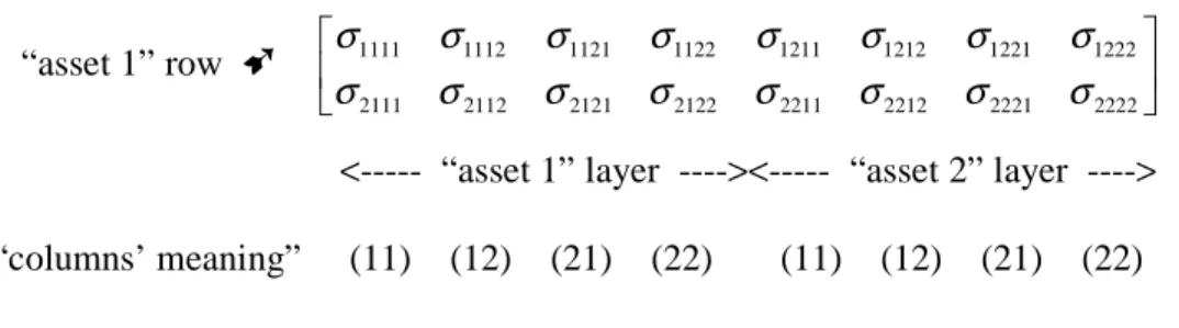
In the case of kurtosis, for instance, two indices/assets must be held constant in each row of a given layer. Calling σijkl a general (co-) kurtosis, when n=2, the final 2 x 8 (=24-1) matrix will result from the juxtaposition of two 2 x 4 (=24-2) layers – one corresponding to the first, and another to the second asset – as shown in Figure 1. Notice that, as pointed out in the figure, the four columns in each layer correspond to ordering the two-by-two combinations, with repetition, of the two assets.
1
Figure 1: Building up the 2 x 8 matrix M4 corresponding to the kurtosis tensor, in the case of two assets (or a two-dimensional random vector):
“asset 1” row ➹ 1111 1112 1121 1122 1211 1212 1221 1222
2111 2112 2121 2122 2211 2212 2221 2222
σ σ σ σ σ σ σ σ
σ σ σ σ σ σ σ σ
<--- “asset 1” layer ----><--- “asset 2” layer ---->
“columns’ meaning” (11) (12) (21) (22) (11) (12) (21) (22)
As happens in a covariance matrix, with the exception of the marginal moments, all other entries in the Mp matrices will share identical values with others in “symmetrical” positions. We shall not pursue this combinatorics here – which can be very important in dealing with special features of the higher moments set -, but only provide a glimpse on its structure, still in the two assets case, in Figure 2.
Figure 2: The general pattern of the 2 x 8 matrix M4 corresponding to the kurtosis tensor, in the case of two assets (each Roman letter corresponds to one of the (three) possible co-kurtoses):
1111
2222
a a b a b b c a b b c b c c
σ
σ
.
Earlier works generalising portfolio choice to higher moments considered only the marginal higher moments of the returns vector, plainly disregarding any co-moment of the same order2. Though the full set of co-moments can quickly become too big – even at the third order -, and simplifying assumptions on its pattern will usually be imposed in practice, it is important to have a way to study the general solution to the problem, irrespective of the simplifying assumptions that might be imposed. In a second step, due consideration of the shape of the higher moments’ structures – which will give way to special patterns of zeroes in our Mp matrices - is a must for grasping a full knowledge of the market one is dealing with.
2
Now suppose that a vector of weights α∈ Rn is given, and x, M2 ,M3 , ...and Mp stand for the matrices, constructed as above, containing the expected (excess) returns, (co-)variances, skewnesses ... and p-moments of a random vector of n assets. The mean return, variance, skewness ... and p-th moment of the portfolio with these weights will be, respectively:
α’x , α’M2α , α’M3 (α⊗α) ... and α’Mp (α⊗α⊗α ... ⊗α)≡α’Mpα⊗p-1 ,
where ‘⊗’ stands for the Kronecker product and α⊗p stands for the (Kronecker) product of vector α by itself, p times .
It is immediate to see that, as real functions of α, all expressions above are homogenous functions of the same degree as the order of the corresponding moment. This means that Euler’s theorem can be easily used in computing derivatives with respect to α. As an example, the derivative of the portfolio kurtosis with respect to the weights will be:
3 4
[αM α ]
α ⊗
∂ ′
∂ = 4M4α⊗3 .
2.2. Solving the classical portfolio problem controlling for skewness and kurtosis.
With the aid of the above notation we shall derive a general solution to the problem of minimising the portfolio variance given a specified set of (expected excess) return, skewness and kurtosis values, for the portfolio.
Consider a portfolio with n risky equities and a riskless asset with rate of return rf . Let [1] stand for a nx1 vector of 1’s and M1 be the vector of the equities’ expected returns and call x = M1 – [1] rf , the vector of mean excess returns. Minimising the variance, for a given mean return, skewness and kurtosis, amounts to finding the solution to the problem:
3 4
, , , 2 , 3
2 1[( ( )p f) ] 2( p 3 ) 3( p 4 )
Min Lα =αM α λ+ E r −r −α x +λ σ −αMα⊗ +λ σ −αM α⊗ , (1)
where M2 , M3 and M4 are, resp., the matrices related to the second, third and fourth
the lambdas are Lagrange multipliers and the three remaining symbols are the α
-portfolio given mean return, skewness and kurtosis.
If R = E(rp) – rf denotes the given excess portfolio return,
the first order conditions (foc) corresponding to (1) are:
2 3
2 1 2 3 2 4
2M α λ= x+3λ M α⊗ +4λ M α⊗
,
R=α x (2)
3
, 2 3
p M
σ =α α⊗
4
, 3 4
p M
σ =α α⊗ .
Multiplying the first expression by the inverse of M2 and then successively
imposing in it each of the three scalar restrictions leads to the system:
1 0 2 2 2 3
2R=λ A +3λ A +4λ A (3)
3 1 2 2 4 3 5
2 3 4
p A A A
σ =λ + λ + λ
4 1 3 2 5 3 6
2σp =λ A +3λ A +4λ A ,
where the new coefficients are:
, 1 0 2
A =x M x− ,
, 1 2 2 2 3
A =x M M− α⊗ ,
, 1 3 3 2 4
A =x M M− α⊗ ,
2 1 2
4 ' 3' 2 3
A =α⊗ M M M− α⊗ , (4)
2 1 3
5 ' 3' 2 4
A =α⊗ M M M− α⊗ ,
3 1 3
6 ' 4' 2 4
System (3) can be solved by a straightforward use of Cramer’s Rule. Substitution of the solution in the expression below, derived from the first foc in (2):
1 1 2 1 3
1 2 2 2 3 2 2 4
2α λ= M − x+3λ M − Mα⊗ +4λ M − M α⊗ (5)
yields the nonlinear system that characterises the optimal weights. The algebra, though not difficult, can be formidable, and use of a symbolic calculator (software) is advisable. We show the explicit final expression in two particular cases:
i) when skewness is not taken into account: calling αK the weights, we have
4 4
6 3 1 0 3 1 3
2 2 4
2 2
0 6 ( 3) 0 6 ( 3)
p p
K K
A R A A A R
M x M M
A A A A A A
σ σ
α = − − + − − α⊗
− − . (6)
ii) when kurtosis is not taken into account: calling αS the weights, we have
3 3
4 2 1 0 2 1 2
2 2 3
2 2
0 4 ( 2) 0 4 ( 2)
p p
S S
A R A A A R
M x M M
A A A A A A
σ σ
α = − − + − − α⊗
− − . (7)
We shall be interested in making comparisons with the classical Markowitz
solution, αM , which does not take into account both skewness and kurtosis. From (5),
and the relevant lines in (2), it is immediately:
1 2 0
M
R M x A
α = − . (8)
Let’s define as ∆S = αS - αM and ∆K = αK - αM , the differences between each
higher moment solution and the Markowitz one. Using (6), (7) and (8), it is not very
3
0 2 1 1 2
2 2 3
2
0 4 2 0
1
( ' )
( )
p
S n S
A A R
M I xx M M
A A A A
σ
α
− − ⊗
−
∆ = −
− , (9)
4
0 3 1 1 3
2 2 4
2
0 6 3 0
1
( ' )
( )
p
K n K
A A R
M I xx M M
A A A A
σ
α
− − ⊗
−
∆ = −
− , (10)
two expressions which, thanks to our notation, reveal themselves to be strikingly
similar. Both can be used as starting points for sensitivity analyses, of the difference
between the respective sets of weights, with respect to either the given value for the
(portfolio) higher moment or a specified (sub)set of the equities’ higher moments.
Nevertheless, such analyses must be carried out with care, as the weights
themselves figure in the r.h.s. of the equations, either explicitly or through the
“numbers” A2, A4or A3, A5. We shall however prove a more fundamental result:
Proposition. Let a given expected return R be fixed and suppose that a higher moment
optimal portfolio (either (6) or (7)) exists THEN if the corresponding higher moment
constraint is binding, the Markowitz solution is never equal to the higher moment
solution.
Proof: we prove for the αK case, the reasoning being identical for αS . Notice first, from
(5) and (6), that if the kurtosis constraint is not biding,
A0σp4 = A R3 ,
and this is enough to make (6) equal to (8). Now suppose the constraint is binding: this
means that the number that multiplies the vector expressed in (10) is non-zero and so
the two solutions can only coincide if the vector itself in (10) is zero. As this vector is
the image of another one, by a positive definite operator, it ensues that
1 3 2 4 0
1
(In xx M' )M K
A α
− ⊗
must be the null vector. As M4αK⊗3≠0 , a little algebra shows this implies that, again,
the higher moment constraint is not binding. As a consequence, the two solutions will
never coincide.
The above proposition gives a more conclusive finish to results as some in Athayde and Flôres (2004), where a complete solution to the three moments portfolio problem is discussed and the (linear) manifold of “common” Markowitz and αS solutions is characterised within the geometric structure of the solutions set in moments space. For the practitioner, it says that – apart from the zero (Lebesgue) measure set where the higher moment constraint is not binding – he will be incurring in error by not considering the higher moment. His “Markowitz weights” will certainly be sub-optimal. But, by how much ?
3. A “one non-zero kurtosis” example.
We shall exploit here the case when the fourth moment is considered, but the structure of the kurtosis tensor has only one non-negligible value, related to the marginal kurtosis of the first asset.
Two remarks are due before pursuing. First, as use of the qualifier “non-negligible” calls attention, kurtoses are usually non-zero3; what is at stake is which ones to consider as relevant, as signalling heavier (than normal) tails. This means that the analyst will be setting to zero all those values for which, taking standardised assets X and Y, for instance, moments like EX4, EY4, EXY3, EX2Y2, etc, won’t be very far from 34. The second is that this very assignment of “zero values” must be made in a consistent way. Considering the same two assets, if one decides not to disregard the two marginal kurtosis, very likely the cross-kurtosis EX2Y2 won’t be possible to be discarded, and – though not necessarily – the same may apply for the pair EXY3, EX3Y. The moral contained in the two remarks is that a much deeper empirical knowledge of the (multivariate) assets distributions is required, for a sensible modelling of the base
3
Though not very common, some co-kurtoses can be negative.
4
higher moments structure. Though this means more additional preparatory work, we consider it positive, as obliging a deeper knowledge of the market.
If only one kurtosis is non-zero, the problem in the previous section simplifies greatly, as the kurtosis constraint in (2) directly supplies the weight of the first asset:
4
1/ 4 1 ( p / 4(1))
α = σ σ , (12)
where the notation used for the relevant kurtosis is self-explanatory. Moreover, the crucial product
3 4
M α⊗ ,
becomes a vector of n-1 zeroes but for the first position, whose ordinate is:
4
3 3 1/ 4 1 4(1) ( p 4(1))
α σ = σ σ ,
a weighted geometric average of the two kurtoses at stake. With these values in hand, one can quickly compute:
4 4
3 1/ 4 3 1/ 2 3 ( p 4(1)) ' .1 6 ( p 4(1)) 11
A = σ σ x m A = σ σ m ,
where m.1 and m11 stand, respectively for the first column and entry of matrix M2-1 = [mij] .
It is now a standard matter to go to expressions (6) and (10) and compute the values of the remaining vector of optimal weights and the vector of differences. We shall concentrate on the latter. After not too cumbersome manipulations, one arrives at the following expression for ∆K :
1 .1
0 .1 .1 2
0 11 .1
'
[ ( ' ) ]
( ' )
K
Rx m
A m x m x A m x m
α −
∆ = −
− . (13)
The above expression conveys two relevant insights:
ii) the influence of the kurtosis considered is through the scalar that multiplies all ordinates of the vector mentioned in i).
As, from (12):
4
1/ 4 1
4(1) 1 4(1) 4(1) 4(1)
1 1
( / )
4 p 4
α σ σ α
σ σ σ
∂ = − = −
∂ , (14)
the sensitivity of the difference with respect to the kurtosis is easily found to be:
1
0 .1 .1 2
4(1) 4(1) 0 11 .1
1
[ ( ' ) ]
4 ( ' )
K A m x m x
A m x m
α
σ∂ ∆ = − σ − =
∂ − , (15)
4
1/ 4
0 .1 .1 5 / 4 2
4(1) 0 11 .1
1 1
[ ( ' ) ]
4 ( ' )
p
A m x m x A m x m
σ σ
= − −
− .
Changes at the vicinity of a given σ4(1) change the signs of the term in (13) which is multiplied by α1 ; moreover, but for a factor of 1/4σ4(1), they are of the same intensity as the term itself. They are also, in absolute terms, directly proportional to the set portfolio kurtosis5, and indirectly, to the non-negligible marginal one.
The last interpretation may be linked to an interesting situation. Suppose the portfolio designer wants to include asset 1 which has a “too” heavy tail. He’s not against heavy tails but wants his portfolio to have a much more moderate one. He’ll then be in the situation of our example, (12) defining a low α1. If this value can be considered quite small with respect to the relevant elements in (13), he’ll design an optimal portfolio distant from the Markowitz one of:
.1
0 .1 .1 2
0 11 .1
'
[ ( ' ) ]
( ' )
K
Rx m
A m x m x A m x m
−
∆ ≅ −
− , (16)
a vector invariant to actual values of both kurtoses, provided their ratio allows to discard the corresponding term in (13). Clearly, if a high R is aimed at, the differences might be rather significant.
Finally, still under this assumption, the difference between the weights allotted to the riskless asset (in the Markowitz less the kurtosis solution) will simply be:
5
.1
0 .1 .1 2
0 11 .1
'
[ ([1]' ) ( ' )([1]' )] ( ' )
Rx m
A m x m x
A m x m
− −
− . (17)
Irrespective of this last case, it is worth reminding that, from (8) and (12), it should be expected that at least the first weight will always be significantly different from the Markowitz one. Anyhow, the set of formulas in this section provides a complete toolkit to analyse the effects of the “one non-zero kurtosis” solution.
4. Concluding remarks.
We have presented explicit formulas for evaluating the difference between Markowitz weights and those from optimal portfolios, with the same given return, considering either asymmetry or kurtosis. We proved that, whenever the higher moment constraint is not binding, the weights are never the same.
If, even by special features of the first and second moments, the difference, though not the null vector, might be negligible, in quite many cases it will be very significant. This is fully exemplified in a simple and appealing case, when the designer wants to incorporate an asset with quite heavy tails, but wants to moderate this effect.
The results add further support that Markowitz weights are not robust to the introduction of higher moments.
References
Athayde, G. M. and R. G. Flôres Jr. 1997. A CAPM with Higher Moments: Theory and Econometrics. EPGE/FGV, Ensaios Econômicos n° 317, Rio de Janeiro.
Athayde, G. M. and R. G. Flôres Jr. 2004. Finding a maximum skewness portfolio – a general solution to three-moments portfolio choice. Journal of Economic Dynamics and Control 28; 1335-52.
Barone-Adesi, G. 1985. Arbitrage equilibrium with skewed asset returns. Journal of Financial and Quantitative Analysis 20; 299-313.
´
Ultimos Ensaios Econˆomicos da EPGE
[547] Fernando de Holanda Barbosa. Dois experimentos de pol´ıtica monet´aria no modelo Novo–Keynesiano. Ensaios Econˆomicos da EPGE 547, EPGE–FGV, Abr 2004.
[548] Samuel de Abreu Pessˆoa, Pedro Cavalcanti Gomes Ferreira, e Fernando A. Ve-loso. The evolution of international output differences (1960–2000): From fac-tors to productivity. Ensaios Econˆomicos da EPGE 548, EPGE–FGV, Jun 2004.
[549] M´arcio Antˆonio Salvato, F´abio Augusto Reis Gomes, e Jo˜ao Victor Issler. Prin-cipais caracter´ısticas do consumo de dur´aveis no Brasil testes de separabilidade entre dur´aveis e n˜ao–dur´aveis. Ensaios Econˆomicos da EPGE 549, EPGE–FGV, Jun 2004.
[550] Jo˜ao Victor Issler e Rachel Couto Ferreira. Avaliando pesquisadores e depar-tamentos de economia no Brasil a partir de citac¸˜oes internacionais. Ensaios Econˆomicos da EPGE 550, EPGE–FGV, Jun 2004.
[551] Humberto Luiz Ataide Moreira e David Martimort.Common agency with infor-med principals. Ensaios Econˆomicos da EPGE 551, EPGE–FGV, Jun 2004.
[552] Luiz Renato Regis de Oliveira Lima e Zhijie Xiao. Purchasing power parity and the unit root tests: A robust analysis. Ensaios Econˆomicos da EPGE 552, EPGE–FGV, Jul 2004.
[553] Daniel Gottlieb, Aloisio Pessoa de Ara´ujo, e Humberto Luiz Ataide Moreira.
A model of mixed signals with applications to countersignaling an the GED. Ensaios Econˆomicos da EPGE 553, EPGE–FGV, Jul 2004.
[554] Lucas J´over Maestri e Carlos Eugˆenio Ellery Lustosa da Costa. The risk– properties of human capital and the design of government policies. Ensaios Econˆomicos da EPGE 554, EPGE–FGV, Jul 2004.
[555] Daniel Gottlieb e Lucas J´over Maestri. Banning information as a redistributive device. Ensaios Econˆomicos da EPGE 555, EPGE–FGV, Jul 2004.
[556] Leonardo Pio Perez e Pedro Cavalcanti Gomes Ferreira. Efeitos macroe-conˆomicos e custos sociais de uma transic¸˜ao entre regimes de previdˆencia no Brasil. Ensaios Econˆomicos da EPGE 556, EPGE–FGV, Jul 2004.
[557] Rubens Penha Cysne. Inflation and income inequality: A link through the job– search process. Ensaios Econˆomicos da EPGE 557, EPGE–FGV, Ago 2004.
[559] Rubens Penha Cysne.Income inequality:The role of impatience in a job–search process. Ensaios Econˆomicos da EPGE 559, EPGE–FGV, Ago 2004.
[560] Rubens Penha Cysne. Towards a measure of income inequality freed from the volatility caused by variations in the rate of unemployment. Ensaios Econˆomicos da EPGE 560, EPGE–FGV, Ago 2004.
[561] Rubens Penha Cysne.On the positive correlation between income inequality and unemployment. Ensaios Econˆomicos da EPGE 561, EPGE–FGV, Ago 2004.
[562] Rubens Penha Cysne. A general–equilibrium closed–form solution to the wel-fare costs of inflation (Forthcoming, Revista Brasileira de Economia). Ensaios Econˆomicos da EPGE 562, EPGE–FGV, Ago 2004.
[563] Marcelo Cˆortes Neri e Marcelo Casal Xerez.Aspectos dinˆamicos de um sistema de metas sociais. Ensaios Econˆomicos da EPGE 563, EPGE–FGV, Ago 2004.
[565] Marcelo Cˆortes Neri e Marcelo Casal Xerez. Desenho de um sistema de metas sociais. Ensaios Econˆomicos da EPGE 565, EPGE–FGV, Set 2004.
[566] Paulo Klinger Monteiro, Rubens Penha Cysne, e Wilfredo Maldonado.Inflation and Income Inequality: A Shopping–Time Aproach (Forthcoming, Journal of Development Economics). Ensaios Econˆomicos da EPGE 566, EPGE–FGV, Set 2004.
[567] Rubens Penha Cysne. Solving the Non–Convexity Problem in Some Shopping– Time and Human–Capital Models. Ensaios Econˆomicos da EPGE 567, EPGE– FGV, Set 2004.
[568] Paulo Klinger Monteiro.First–Price auction symmetric equlibria with a general distribution. Ensaios Econˆomicos da EPGE 568, EPGE–FGV, Set 2004.
[569] Samuel de Abreu Pessˆoa, Fernando A. Veloso, e Pedro Cavalcanti Ferreira. On The Tyranny of Numbers: East Asian Miracles in World Perspective. Ensaios Econˆomicos da EPGE 569, EPGE–FGV, Out 2004.
[570] Rubens Penha Cysne. On the Statistical Estimation of Diffusion Processes – A Partial Survey (Revised Version, Forthcoming Brazilian Review of Econome-trics). Ensaios Econˆomicos da EPGE 570, EPGE–FGV, Out 2004.
[571] Aloisio Pessoa de Ara´ujo, Humberto Luiz Ataide Moreira, e Luciano I. de Cas-tro Filho.Pure strategy equilibria of multidimensional and Non–monotonic auc-tions. Ensaios Econˆomicos da EPGE 571, EPGE–FGV, Nov 2004.