ПАЛАТА ЛОРДОВ ВЕЛИКОБРИТАНИИ: ИЗ СРЕДНЕВЕКОВЬЯ В XXI ВЕК

МЕЖДУНАРОДНЫЙ

НАУЧНО-ИССЛЕДОВАТЕЛЬСКИЙ ЖУРНАЛ

ISSN 2303-9868

Meždunarodnyj

naučno-issledovatel'skij

žurnal

№ 9 (28) 2014

Периодический теоретический и научно-практический журнал. Выходит 12 раз в год.

Учредитель журнала: ИП Соколова М.В. Главный редактор: Миллер А.В.

Адрес редакции: 620075, г. Екатеринбург, ул. Красноармейская, д. 4, корп. А, оф. 17.

Электронная почта: editors@research-journal.org

Сайт: www.research-journal.org

Подписано в печать 08.10.2014. Тираж 900 экз.

Заказ 19344.

Отпечатано с готового оригинал-макета.

Отпечатано в типографии ООО "Компания ПОЛИГРАФИСТ" 623701, г. Березовский, ул. Театральная, дом № 1, оф. 88.

Сборник по результатам XXXI заочной научной конференции Research Journal of International

Studies.

За достоверность сведений, изложенных в статьях, ответственность несут авторы. Полное

или частичное воспроизведение или размножение, каким бы то ни было способом материалов,

опубликованных в настоящем издании, допускается только с письменного разрешения авторов.

Номер свидетельства о регистрации в Федеральной Службе по надзору в сфере связи,

информационных технологий и массовых коммуникаций: ПИ № ФС 77 – 51217.

Члены редколлегии:

Филологические науки: Растягаев А.В. д-р филол. наук, Сложеникина Ю.В. д-р филол. наук, Штрекер Н.Ю. к.филол.н., Вербицкая О.М. к.филол.н. Технические науки: Пачурин Г.В. д-р техн. наук, проф., Федорова Е.А. д-р техн. наук, проф., Герасимова Л.Г., д-р техн. наук, Курасов В.С., д-р техн. наук, проф., Оськин С.В., д-р техн. наук, проф.

Педагогические науки: Лежнева Н.В. д-р пед. наук, Куликовская И.Э. д-р пед. наук, Сайкина Е.Г. д-р пед. наук, Лукьянова М.И. д-р пед. наук. Психологические науки: Мазилов В.А. д-р психол. наук, Розенова М.И., д-р психол. наук, проф., Ивков Н.Н. д-р психол. наук.

Физико-математические науки: Шамолин М.В. д-р физ.-мат. наук, Глезер А.М. д-р физ.-мат. наук, Свистунов Ю.А., д-р физ.-мат. наук, проф. Географические науки: Умывакин В.М. д-р геогр. наук, к.техн.н. проф., Брылев В.А. д-р геогр. наук, проф., Огуреева Г.Н., д-р геогр. наук, проф. Биологические науки: Буланый Ю.П. д-р биол. наук, Аникин В.В., д-р биол. наук, проф., Еськов Е.К., д-р биол. наук, проф., Шеуджен А.Х., д-р биол. наук, проф.

Архитектура: Янковская Ю.С., д-р архитектуры, проф.

Ветеринарные науки: Алиев А.С., д-р ветеринар. наук, проф., Татарникова Н.А., д-р ветеринар. наук, проф. Медицинские науки: Медведев И.Н., д-р мед. наук, д.биол.н., проф., Никольский В.И., д-р мед. наук, проф.

Исторические науки: Меерович М.Г. д-р ист. наук, к.архитектуры, проф., Бакулин В.И., д-р ист. наук, проф., Бердинских В.А., д-р ист. наук, Лёвочкина Н.А., к.иси.наук, к.экон.н.

Культурология: Куценков П.А., д-р культурологии, к.искусствоведения. Искусствоведение: Куценков П.А., д-р культурологии, к.искусствоведения.

Философские науки: Петров М.А., д-р филос. наук, Бессонов А.В., д-р филос. наук, проф.

Юридические науки: Грудцына Л.Ю., д-р юрид. наук, проф., Костенко Р.В., д-р юрид. наук, проф., Камышанский В.П., д-р юрид. наук, проф., Мазуренко А.П. д-р юрид. наук, Мещерякова О.М. д-р юрид. наук, Ергашев Е.Р., д-р юрид. наук, проф.

Сельскохозяйственные науки: Важов В.М., д-р х. наук, проф., Раков А.Ю., д-р х. наук, Комлацкий В.И., д-р х. наук, проф., Никитин В.В. д-р с.-х. наук, Наумкин В.П., д-р с.-с.-х. наук, проф.

Социологические науки: Замараева З.П., д-р социол. наук, проф., Солодова Г.С., д-р социол. наук, проф., Кораблева Г.Б., д-р социол. наук. Химические науки: Абдиев К.Ж., д-р хим. наук, проф., Мельдешов А. д-р хим. наук.

Науки о Земле: Горяинов П.М., д-р геол.-минерал. наук, проф.

Экономические науки: Бурда А.Г., д-р экон. нау, проф., Лёвочкина Н.А., д-р экон. наук, к.ист.н., Ламоттке М.Н., к.экон.н. Политические науки: Завершинский К.Ф., д-р полит. наук, проф.

Фармацевтические науки: Тринеева О.В. к.фарм.н., Кайшева Н.Ш., д-р фарм. наук, Ерофеева Л.Н., д-р фарм. наук, проф.

Оглавление

ФИЗИКО-МАТЕМАТИЧЕСКИЕ НАУКИ / PHYSICS AND MATHEMATICS

5

FINITE

ELEMENT

MESH

AUTOMATIC

GENERATION

USING

TRIANGULAR

SUBDIVISION

SCHEMES

5

ON

TOPOLOGICAL

METHODS

IN

SHAPE

MODELING

7

ПРЕПОДАВАНИЕ

ФИНАНСОВЫХ

ВЫЧИСЛЕНИЙ

В

EXCEL

НА

АНГЛИЙСКОМ

ЯЗЫКЕ

13

THE

BIG

BANG

THEORY

AND

UNIVERSE

MODELING.MISTAKES

IN

THE

RELATIVITY

THEORY

15

БИОЛОГИЧЕСКИЕ НАУКИ / BIOLOGY

19

ФИТОЭКОЛОГИЧЕСКАЯ

ПАСПОРТИЗАЦИЯ

САМАРСКИХ

ГОРОДСКИХ

ПАРКОВ

19

ПРОСТРАНСТВЕННАЯ

СИНХРОНИЗАЦИЯ

КОРКОВЫХ

ПОТЕНЦИАЛОВ

АЛЬФА-ДИАПАЗОНА

ЭЭГ

ПОСЛЕ

ДЕЙСТВИЯ

СИГНАЛОВ

ТИПА

GO/NOGO

В

ИССЛЕДОВАНИЯХ

УСТАНОВКИ

НА

ЛИЦЕВУЮ

ЭКСПРЕССИЮ

21

ТЕХНИЧЕСКИЕ НАУКИ / ENGINEERING

24

АДАПТИВНАЯ

БЫСТРОДЕЙСТВУЮЩАЯ

ЗАЩИТА

НИЗКОВОЛЬТНЫХ

КОМПЛЕКТНЫХ

РАСПРЕДУСТРОЙСТВ

24

ДОРОЖНАЯ

СЕТЬ

СВЕРДЛОВСКОЙ

ОБЛАСТИ

26

НЕТРАДИЦИОННОЕ

СЫРЬЕ

ДЛЯ

СТЕНОВЫХ

МАТЕРИАЛОВ

27

ПОЛИМЕРНЫЕ

КОМПОЗИЦИОННЫЕ

МАТЕРИАЛЫ

ДЛЯ

АВИАЦИОННОЙ

И

КОСМИЧЕСКОЙ

ТЕХНИКИ

29

КОМПОЗИЦИОННЫЕ

МАТЕРИАЛЫ

НА

ОСНОВЕ

ПОЛИИМИДНОЙ

МАТРИЦЫ

ДЛЯ

КОСМИЧЕСКИХ

ЛЕТАТЕЛЬНЫХ

АППАРАТОВ

30

СПОСОБ

ЗАЩИТЫ

АВТОМАТИЗИРОВАННЫХ

СИСТЕМ

31

РАДИАЦИОННАЯ

ЗАЩИТА

КОСМИЧЕСКИХ

ЯДЕРНЫХ

ЭНЕРГЕТИЧЕСКИХ

УСТАНОВОК

35

АНТИКОРРОЗИЙНАЯ

ОБРАБОТКА

ЯДЕРНОГО

ЭНЕРГЕТИЧЕСКОГО

ОБОРУДОВАНИЯ

36

НОВЫЕ

ПОДХОДЫ

В

ТЕХНОЛОГИИ

СОЗДАНИЯ

КОМПОЗИЦИОННЫХ

МАТЕРИАЛОВ

37

ТЕРМОСТОЙКИЕ

ПОЛИМЕРНЫЕ

КОМПОЗИТЫ

ДЛЯ

НЕЙТРОННОЙ

И

ГАММА-ЗАЩИТЫ

39

РАДИАЦИОННО-ЗАЩИТНЫЙ

КОНСТРУКЦИОННЫЙ

КОМПОЗИЦИОННЫЙ

МАТЕРИАЛ

40

СПОСОБ

КОНТРОЛЯ

ПОЛОЖЕНИЯ

ЕМКОСТИ

С

РАСПЛАВОМ

41

СЕРПЕНТИНИТОВЫЙ

ЗАПОЛИТЕЛЬ

ДЛЯ

РАДИАЦИОННО-ЗАЩИТНОГО

БЕТОНА

44

РЕЗУЛЬТАТЫ

ТЕРМОЦИКЛИРОВАНИЯ

РАДИАЦИОННО-ЗАЩИТНОГО

МЕТАЛЛОКОМПОЗИЦИОННОГО

МАТЕРИАЛА

45

МОДЕЛИРОВАНИЕ

ПРОХОЖДЕНИЯ

ЭЛЕКТРОНОВ

ЧЕРЕЗ

КОМПОЗИЦИОННЫЙ

МАТЕРИАЛ

НА

ОСНОВЕ

АЛЮМИНИЯ

46

РАДИАЦИОННО-СТОЙКИЙ

КОНСТРУКЦИОННЫЙ

КОМПОЗИТ

ДЛЯ

БИОЛОГИЧЕСКОЙ

ЗАЩИТЫ

ЯДЕРНЫХ

РЕАКТОРОВ

47

НАПОЛНИТЕЛЬ

В

ПОЛИМЕРЫ

ДЛЯ

ОБЕСПЕЧЕНИЯ

РАДИАЦИОННОЙ

ЗАЩИТЫ

48

РАДИАЦИОННО-ЗАЩИТНЫЕ

ДИЭЛЕКТРИЧЕСКИЕ

КОМПОЗИТЫ

ДЛЯ

КОСМИЧЕСКИХ

СИСТЕМ

49

РАЗРАБОТКА

КОМПОЗИЦИОННЫХ

МАТЕРИАЛОВ,

УПРОЧНЁННЫХ

ВКЛЮЧЕНИЯМИ

ТВЕРДОГО

СПЛАВА 50

ИССЛЕДОВАНИЕ

АДГЕЗИОННОЙ

ПРОЧНОСТИ

ТЕРМОРЕГУЛИРУЮЩЕГО

ПОКРЫТИЯ

52

УСТАНОВКА

ДЛЯ

СПЕЦИАЛЬНЫХ

ИСПЫТАНИЙ

ДИЭЛЕКТРИКОВ

ВЫСОКОЭНЕРГЕТИЧЕСКИМ

ЭЛЕКТРОННЫМ

ИЗЛУЧЕНИЕМ

53

ЭКСПЕРИМЕНТАЛЬНЫЕ

И

РАСЧЕТНЫЕ

КОЭФФИЦИЕНТЫ

ОСЛАБЛЕНИЯ

ГАММА-ИЗЛУЧЕНИЯ

КОМПОЗИТА

54

ТЕХНОЛОГИЯ

ФОРМОВАНИЯ

ПОЛИМЕРНЫХ

КОМПОЗИТОВ

НА

ОСНОВЕ

ФТОРОПЛАСТА

55

ИССЛЕДОВАНИЕ

И

РАЗРАБОТКА

ПЕРСПЕКТИВНЫХ

МЕТОДОВ

ОПТИМИЗАЦИИ

БОРТОВЫХ

РАСПРЕЖЕЛЕННЫХ

СИСТЕМ

УПРАВЛЕНИЯ

РЕАЛЬНОГО

ВРЕМЕНИ

56

СЕЛЬСКОХОЗЯЙСТВЕННЫЕ НАУКИ / AGRICULTURAL SCIENCES

59

ВЛИЯНИЕ

ОРГАНИЧЕСКИХ

УДОБРЕНИЙ

НА

СОДЕРЖАНИЕ

В

ПОЧВЕ

ПОДВИЖНОГО

ФОСФОРА

59

ВЛИЯНИЕ

РЕГУЛЯТОРОВ

РОСТА

И

ДЕСИКАНТОВ

НА

УРОЖАЙНОСТЬ

И

КАЧЕСТВО

СЕМЯН

САХАРНОГО

СОРГО

60

ДИНАМИКА

РОСТА

И

НАЧАЛО

РЕПРОДУКТИВНОГО

РАЗВИТИЯ

СОСНЫ

КЕДРОВОЙ

СИБИРСКОЙ

21-30-ЛЕТНЕГО

ВОЗРАСТА

НА

ПЛАНТАЦИИ

«ИЗВЕСТКОВАЯ»

62

ИСТОРИЧЕСКИЕ НАУКИ / HISTORY

65

ДЕЯТЕЛЬНОСТЬ

ОБЛАСТНОЙ

ОРГАНИЗАЦИИ

КОММУНИСТИЧЕСКОЙ

ПАРТИИ

СОВЕТСКОГО

СОЮЗА

ПО

АКТИВИЗАЦИИ

ОБЩЕСТВЕННО-ПОЛИТИЧЕСКОЙ

ЖИЗНИ

НАСЕЛЕНИЯ

АСТРАХАНСКОЙ

ОБЛАСТИ

В

1965-1985

65

УЧАСТИЕ

ОБЛАСТНОЙ

КОМСОМОЛЬСКОЙ

ОРГАНИЗАЦИИ

АСТРАХАНСКОЙ

ОБЛАСТИ

В

РАЗВИТИИ

РЕГИОНА

68

ПАЛАТА

ЛОРДОВ

ВЕЛИКОБРИТАНИИ:

ИЗ

СРЕДНЕВЕКОВЬЯ

В

XXI

ВЕК

70

ГОРОДСКОЕ

ПЛАНИРОВАНИЕ

ИНДУСТРИАЛЬНОГО

ГОРОДА

В

ПЕРИОД

ПРОМЫШЛЕННОГО

РОСТА

КОНЦА

20-30-Х

ГОДОВ

XX

ВЕКА

(НА

МАТЕРИАЛАХ

ГОРОДА

КАЗАНИ)

72

ЭКОНОМИЧЕСКИЕ НАУКИ / ECONOMICS

73

МОБИЛЬНЫЕ

ТЕХНОЛОГИИ

РЕСТОРАННОГО

БИЗНЕСА

73

НАЦИОНАЛЬНАЯ

ПЛАТЕЖНАЯ

СИСТЕМА

С

НУЛЯ

–

ПЛЮСЫ

И

МИНУСЫ

74

ВЗАИМОСВЯЗЬ

ПОКАЗАТЕЛЕЙ

ДИВЕРСИФИКАЦИИ

ДЕЯТЕЛЬНОСТИ

ПРЕДПРИЯТИЯ

И

ЕГО

УСТОЙЧИВОСТИ

75

ЛОГИСТИКА

МОБИЛЬНОЙ

ТОРГОВЛИ

77

К

ВОПРОСУ

О

ВЗАИМОСВЯЗИ

ПОНЯТИЙ

«РИСК»,

«НЕОПРЕДЕЛЕННОСТЬ»,

«ВЕРОЯТНОСТЬ»

78

ХАРАКТЕРИСТИКА

МИРОВОГО

ОПЫТА

РЕФОРМИРОВАНИЯ

БУХГАЛТЕРСКОГО

УЧЕТА

79

ОСНОВЫ

РИСК-МЕНЕДЖМЕНТА

80

ПРИНЯТИЕ

УПРАВЛЕНЧЕСКИХ

РЕШЕНИЙ

В

УСЛОВИЯХ

КРИЗИСА

82

СРАВНИТЕЛЬНАЯ

ХАРАКТЕРИСТИКА

КРИТЕРИЕВ

ПРИЗНАНИЯ

ЭЛЕМЕНТОВ

ФИНАНСОВОЙ

ОТЧЕТНОСТИ

В

БУХГАЛТЕРСКОМ

И

НАЛОГОВОМ

УЧЕТЕ

83

ЗНАЧЕНИЕ

ИНСТРУМЕНТОВ

МОНЕТАРНОЙ

ПОЛИТИКИ

В

ЭКОНОМИКЕ

СТРАНЫ

85

ОСОБЕННОСТИ

НОРМАТИВНО-ПРАВОВОГО

РЕГУЛИРОВАНИЯ

БУХГАЛТЕРСКОГО

УЧЕТА

В

СЕЛЬСКОМ

ХОЗЯЙСТВЕ

86

ХАРАКТЕРИСТИКА

МЕТОДОВ

ТРАНСФОРМАЦИИ

ФИНАНСОВОЙ

ОТЧЕТНОСТИ

В

СООТВЕТСТВИИ

С

ТРЕБОВАНИЯМИ

МЕЖДУНАРОДНЫХ

СТАНДАРТОВ

88

ИССЛЕДОВАНИЕ

ВИДОВ

НЕОПРЕДЕЛЕННОСТИ

89

ОЦЕНКА

НЕОПРЕДЕЛЕННОСТИ

ДЕЛОВОЙ

СРЕДЫ

НА

ПРИМЕРЕ

ООО

«НПК

«ЭНЕРГИЯ»

90

РАЗРАБОТКА

АЛГОРИТМА

ФОРМИРОВАНИЯ

ПРОДУКТОВОГО

ПОРТФЕЛЯ

91

ЗАДАЧИ

УПРАВЛЕНИЯ

ПЕРСОНАЛОМ

ПРИ

РАЗРАБОТКЕ

И

РЕАЛИЗАЦИИ

ПРОЕКТОВ

93

МЕТОДЫ

ОЦЕНКИ

ИНВЕСТИЦИОННОГО

КЛИМАТА

РЕГИОНА

94

ПОЗИЦИЯ

РОССИИ

В

ИННОВАЦИОННЫХ

РЕЙТИНГАХ

В

2014

ГОДУ

97

ФИЛОЛОГИЧЕСКИЕ НАУКИ / PHILOLOGY

99

БИБЛЕИЗМЫ

И

КОРАНИЧЕСКИЕ

ФРАЗЕОЛОГИЗМЫ

В

РУССКОМ

И

ТУРЕЦКОМ

ЯЗЫКАХ

99

ТЕМАТИЧЕСКАЯ

ПАЛИТРА

КРЫМСКОТАТАРСКОЙ

ПОЭЗИИ

ПЕРИОДА

ПРОБУЖДЕНИЯ

(1883-1917

ГГ.). 100

DISCOURSE

OF

SCOUTING:

CATEGORIZATION

AND

TYPOLOGY

102

ЕЩЁ

РАЗ

К

ВОПРОСУ

О

МАНИПУЛЯТИВНЫХ

РЕЧЕВЫХ

СТРАТЕГИЯХ

(НА

МАТЕРИАЛЕ

БРИТАНСКИХ

СМИ)

103

ДИМИНУТИВЫ

В

КРУГУ

БАЗОВЫХ

ЭМОЦИЙ

(НА

ПРИМЕРЕ

"DIE

SCHÖNSTEN

DEUTSCHEN

ERZÄHLUNGEN")

105

ЮРИДИЧЕСКИЕ НАУКИ / JURISPRUDENCE

107

ПРОБЛЕМЫ,

ВОЗНИКАЮЩИЕ

В

ХОДЕ

ОСУЩЕСТВЛЕНИЯ

ГОСУДАРСТВЕННОГО

СТРОИТЕЛЬНОГО

НАЛЗОРА,

И

ПУТИ

ИХ

РЕШЕНИЯ

107

ПЕДАГОГИЧЕСКИЕ НАУКИ / PEDAGOGY

109

ПОДГОТОВКА

ПРОФЕССИОНАЛЬНОГО

СПЕЦИАЛИСТА

В

КОНТЕКСТЕ

КОМПЕТЕНТНОСТНОГО

ПОДХОДА 109

СОДЕРЖАТЕЛЬНАЯ

СУЩНОСТЬ

ФИЗИЧЕСКОГО

ВОСПИТАНИЯ

СТУДЕНТОВ,

БОЛЬНЫХ

ОЖИРЕНИЕМ,

В

СПЕЦИАЛЬНЫХ

МЕДИЦИНСКИХ

ГРУППАХ

ВУЗОВ

111

ОПРЕДЕЛЕНИЕ

УРОВНЯ

ОБЩИТЕЛЬНОСТИИ

И

«ПОМЕХ»

В

УСТАНОВЛЕНИИ

ЭМОЦИОНАЛЬНЫХ

КОНТАКТОВ

115

ТЕХНОЛОГИЯ

ПРОВЕДЕНИЯ

УЧЕБНО-ТРЕНИРОВОЧНЫХ

ЗАНЯТИЙ

С

ЛЮДЬМИ

ИМЕЮЩИХ

ПРОБЛЕМЫ

И

ПАТОЛОГИЧЕСКИЕ

ОТКЛОНЕНИЯ

В

ФУНКЦИЯХ

ОПОРНО-ДВИГАТЕЛЬНОГО

АППАРАТА

116

ФОРМИРОВАНИЕ

ДВИГАТЕЛЬНЫХ

УМЕНИЙ

СТУДЕНТОВ

ИНСТИТУТОВ

ФИЗИЧЕСКОЙ

КУЛЬТУРЫ

В

МЕДЕЦИНСКИЕ НАУКИ / MEDICINE

123

ИЗМЕНЕНИЕ

АНГИОАРХИТЕКТОНИКИ

ТОНКОЙ

КИШКИ

В

ДИНАМИКЕ

ПРИ

ОПЕРАТИВНЫХ

ВМЕШАТЕЛЬСТВАХ

НА

ПОЗВОНОЧНИКЕ

(ЭКСПЕРИМЕНТАЛЬНОЕ

ИССЛЕДОВАНИЕ)

123

АНАЛИЗ

КЛИНИЧЕСКИХ

СИМПТОМОВ

ГИПОВИТАМИНОЗА

С

ОТ

РАЦИОНА

ПИТАНИЯ

У

СТУДЕНТОВ

ВУЗОВ

Г.

МИНСКА.

126

РАЗВИТИЕ

ПЛАЦЕНТАРНОЙ

НЕДОСТАТОЧНОСТИ

НА

ФОНЕ

НАРУШЕНИЙ

СИСТЕМЫ

ГЕМОСТАЗА

У

БЕРЕМЕННЫХ

С

ХРОНИЧЕСКИМИ

ЗАБОЛЕВАНИЯМИ

ПЕРИФЕРИЧЕСКИХ

ВЕН

129

ПСИХОЛОГИЧЕСКИЕ НАУКИ / PSYCOLOGY

131

СПЕЦИФИКА

ЦЕННОСТНЫХ

ОРИЕНТАЦИЙ

ПРАКТИЧЕСКИХ

ПСИХОЛОГОВ

СИСТЕМЫ

ОБРАЗОВАНИЯ

В

ПРОЦЕССЕ

ПРОФЕССИОНАЛЬНОГО

ОБУЧЕНИЯ

131

НЕЙРОГЕНЕТИЧЕСКИЙ

КОНТЕКСТ

ЭВОЛЮЦИОННО-ИСТОРИЧЕСКОЙ

МОДЕЛИ

ТРЕВОГИ

133

СОЦИОЛОГИЧЕСКИЕ НАУКИ / SOCIOLOGY

135

ОСНОВНЫЕ

ОПРЕДЕЛЕНИЯ

ОРГАНИЗАЦИОННОЙ

КУЛЬТУРЫ

135

ИННОВАЦИОННЫЕ

МЕТОДЫ

ОБУЧЕНИЯ

КАК

СПОСОБЫ

АКТИВИЗАЦИИ

МЫСЛИТЕЛЬНОЙ

ДЕЯТЕЛЬНОСТИ

СТУДЕНТОВ

136

КУЛЬТУРОЛОГИЯ / CULTURE STUDIES

139

СОЦИОКУЛЬТУРНЫЙ

КОД

КАК

СИСТЕМООБРАЗУЮЩИЙ

ФАКТОР

СТРУКТУРИРОВАНИЯ

И

ФИЗИКО-МАТЕМАТИЧЕСКИЕ НАУКИ / PHYSICS AND MATHEMATICS

Берзин Д.В.

Кандидат физико-математических наук, доцент, Финансовый университет при Правительстве Российской Федерации, Москва ПОСТРОЕНИЕ FE СЕТИ ПОСРЕДСТВОМ ТРЕУГОЛЬНЫХ ПОДРАЗБИЕНИЙ

Аннотация В работе предложен новый алгоритм для построения треугольной сети для поверхности NURBS, заданной посредством контрольных точек. При этом используются две техники подразбиений – Modified Butterfly и Loop.

Ключевые слова: NURBS, контрольные точки, система автоматизированного проектирования, треугольная сеть,

подразбиения.

Berzin D.V.

PhD, Associate Professor,Financial University under the Government of the Russian Federation, Moscow FINITE ELEMENT MESH AUTOMATIC GENERATION USING TRIANGULAR SUBDIVISION SCHEMES

Abstract We suggest here a new algorithm for triangular finite element mesh generation for NURBS surface represented as a set of control points. We use a modern approach – subdivision techniques, which has many advantages. Two different subdivision schemes are presented here: Modified Butterfly and Loop ones.

Keywords: NURBS, control points, CAD system, FE mesh, subdivision. 1. The problem to solve

Suppose we are given a 2-dimensional surface S, defined by means of control points, for example, by data stored in IGES file type 126 [1]. Thus, we have a set of control points d̲̲̲ ̲ ̲ ̲ ̲ ̲ ̲ ̳ ̳ ̲_ij, weights w_ij , knot sequence (u_n,v_k), where i= -1, … , L+1; j=-1, … , M+1; n=0, …, L; k=0, … , M. And the corresponding NURBS surface has the following parametric form:

s(u,v) =

3 3

3 3

( ) ( )

( ) ( )

ij ij i j i j

ij i j

i j

w d N u N v

w N u N v





,

where N3_i(u), N3_j(v) are B-spline functions ([2], Ch.10,17).

Triangular patches in CAD system development have certain advantages over quadrilateral ones ([2], Ch.24). For example, they do not suffer from some kinds of degeneracies and are thus better suited to describe complex geometries than are rectangular patches.

Our task is to construct a triangular finite element mesh satisfying the conditions ([3], [4], [5]):

Triangles should satisfy an aspect ratio, i.e. they must be close to regular triangles. Nodes of triangles must lie exactly on the given surface S. The distance d between triangle and surface should be less than number



, chosen by a user. User should be able to change the mesh adaptively (e.g., density of the mesh in some areas, the number



, and so on).

2. Solution of the problem

Without loss of generality, consider a bicubic B-spline surface S.

Step 1. Bringing a bicubic B-spline surface into a piecewise bicubic Bezier form. This is a standard CAGD procedure ([2], Ch.17), and can be realized by a subroutine, say, “Bezier”. Suppose, now we are given a rectangular net of points b_0,0, … , b_{3 ,3L M} . All of them lie on S . Consider a planar rectangular domain R , spanned on points A_nk, that there is a homeomorphism

g: R



S, g( A_nk) = b_{3 ,3n k}.

Remark. In general case there is a polyhedron K instead of rectangle R, K



R4 ([5], Ch.3).

Step 2. To construct an initial mesh, we pick out points from the set {b_{3 ,3n k}}. We want the initial mesh to be close to the aspect ratio demand. The subroutine, say, “Initial” uses diagonal transpose technique (e.g., see [4]): it starts from the rectangle A₀₀A₀₁A₁₀A₁₁, compares b_0,0b_3,3 and b_0,3b_3,0, and chooses the shortest diagonal to divide a quadrilateral into 2 triangles. My colleague Nikita Kojekine (see also [8] and [9]) wrote a computer program in C++ to get the results. The program divides each quadrilateral in the same way.

4. Subdivision process

Step 3a. For a subdivision process, we suggest an interpolating Modified Butterfly scheme ([6], Ch.4). We can suppose here that, loosely speaking, the subdivision surfaces f_k(R) approach to a given surface S. Here f_k



f , and f (R) is the subdivision surface. After k-th step of subdivision, we obtain a triangular net {B_ijk }



R, and a corresponding mesh {bk_ij }, where

f (B_ijk) = b_ijk, g(B_ij)



{b0_ij }, k=0,1, … .

A user can interactively choose a level of subdivision in different domains. Let the subroutine be called “Subdivision”.

Step 3b. Instead of Modified Butterfly scheme, sometimes it is advantageous to use other triangular schemes. One of most popular of them is (approximating) Loop scheme ([6], Ch.4). The explanation and results for the step 3 follows:

Program “Subdivision”. The program “subdivision surfaces” was created to demonstrate two different triangular subdivision schemes. One is interpolating Modified-Butterfly scheme, second is Loop scheme. The program was written in Microsoft Visual C++ using MFC (Microsoft Foundation Classes) technology, OpenGL and VTK (free-source visualization toolkit) by my colleague Nikita Kojekine. Program reads initial mesh files first. The very simple format was developed for them.

Fig. 1 - Tetrahedron interpolated using Modified Butterfly Scheme, after 6 steps subdivisions

Fig. 2 - Same tetrahedron approximated using Loop scheme, after 6 steps of subdivision

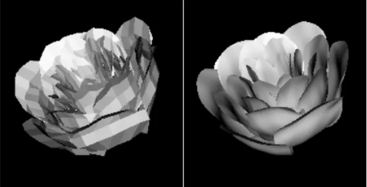
The program is provided with more complex examples of meshes. For example, the ‘rose’ initial mesh and after subdivision:

Fig. 3 - Rose. Initial mesh on the left, and approximated image to the right. 3 steps of subdivision using Loop scheme

Another addition to "subdivision" program can be used to demonstrate the interpolation of colors using Modified Butterfly scheme too. Let us look at the same example with tetrahedron:

Step 4. After k-th level of subdivision we project (by a subroutine, say, “Projection”) a mesh {b_ijk } onto the surface S. Let ak_ij= P(b_ijk) ,

where P is a projection, ak_ij



S.

Step 5. Now one should verify a condition 3). We suggest here to use a distance d₁ between a barycenter of corresponding triangle and S (instead of d), and verify a condition d₁<



/2. Let the subroutine be called “Distance”. For the mesh to be conforming, we can use a method from [7] for dividing big triangles into several smaller ones.

References 1. “Fuji technical research” company. Private communications, Tokyo, 2000. 2. Gerald Farin “Curves and surfaces for CAGD”. Academic press, 1993.

3. Ichiro Hagiwara. Private communications, Tokyo Institute of Technology, 2000.

4. Ho-Le K. “Finite element mesh generation methods: review and classification”. Computer-Aided Design, 20:27-38, 1988 5. K.-J. Bathe “Finite Element Procedures”. Prentice-Hall, 1996

6. “Subdivision for Modeling and Animation”. SIGGRAPH 99 Course Notes.

7. Rivara M.C. “Algorithms for refining triangular grids suitable for adaptive and multi-grid techniques”. Int. J. Numer. Meth. Eng. Vol 20 (1984) pp. 745-756.

8. Dmitry Berzin "Finite element mesh generation using subdivision technique" // Research Journal of International Studies, №8 (27) 2014, p. 6

9. Dmitry Berzin "Finite element automatic mesh generation using Modified Butterfly subdivision scheme" // Research Journal of International Studies, №8 (27) 2014, p. 8

Берзин Д.В.

Кандидат физико-математических наук, доцент, Финансовый университет при Правительстве Российской Федерации, Москва О ТОПОЛОГИЧЕСКИХ МЕТОДАХ В ПРОСТРАНСТВЕННОМ МОДЕЛИРОВАНИИ

Аннотация Существует множество хороших работ, касающихся геометрических методов пространственного моделирования. Но очень немногие исследования затрагивали топологический аспект. В настоящей работе мы предлагаем краткий обзор базовых топологических концепций в пространственном моделировании.

Ключевые слова: симплициальные комплексы, гомотопия, клеточные пространства, гомеоморфизм. Berzin D.V.

PhD, Associate Professor,Financial University under the Government of the Russian Federation, Moscow ON TOPOLOGICAL METHODS IN SHAPE MODELING

Abstract There are many excellent research results on geometrical shape modeling. As for the topological level of the modeling, limited researches have been conducted. In this paper we overview some basic concepts of topology, which can be applied to shape modeling.

Keywords: simplicial complex, cell space, homeomorphism 1. Introduction

The notions of topological space and homeomorphism are ones of fundamental in mathematics. Roughly speaking, homeomorphisms describe objects deformations, and the concept of homeomorphism is useful for discovering important properties of objects, that are not changing under such deformations. These properties are called topological, in contrast to metrical ones, which are connected with distances between points, angles between lines and so on. For example, cube and tetrahedron are different from metrical point of view, but they are homeomorphic. Subtle metric properties are not important for many problems, and it is needed to reveal “rough” topological properties. Topology (in particular, homotopy topology) is an important branch of mathematics (e.g., see [1], [2]). Its basic concepts, useful for shape modeling, are homeomorphism, homotopy, simplicial complex, cell space.

It is known, that the concept of manifold is a fundamental in geometry. Structure and properties of smooth manifolds give us a good basis for computer-aided geometrical design (CAGD) and computer graphics (CG) methods. For example, Gaussian curvature and other invariants are of a great importance in geometric modeling. It appears that sometimes a structure of a smooth manifold is not sufficient, so the notion of simplicial complex or cellular space is necessary. Simplicial complex can be regarded as a triangulated object (manifold or non-manifold). A cellular space is an object, constructed from some primitives – cells, and can be regarded as generalization of the notion “smooth manifold”.

Triangulations of subdivided manifolds (and non-manifolds) are used extensively in solid modeling. Paoluzzi et al. [3] provide an overview of related work and analyze the benefits of representing such triangulations using simplicial complexes. Bertolotto et al. [4] present hierarchical simplicial representations for subdivided objects, but these do not support changes of topological type. Polyhedra can also be represented using more general representations. The simplicial set representation of Lang and Lienhardt [5] generalizes simplicial complexes to allow incomplete and degenerate simplices. Cell complexes (i.e. cell spaces), formed by subdividing manifolds into non-simplicial cells, can be represented using radial edge structure [6] or the cell tuple structure [7]. Kunii et al. [8-14] and [23] used so-called cellular approach for shape modeling. The authors give a definition of homotopy and cellular space, and examples of cellular decompositions of geometric objects together with corresponding attaching maps as well. The progressive simplicial complex (PSC) representation for geometrical objects was described in [15]. The PSC representation expresses an arbitrary triangulated model M (e.g. any dimension, orientable, non-manifold) as the result of successive refinements applied to the base model M1 that always consists of a single vertex. Thus both geometric and topological complexities are recovered progressively. Combinatorial and topological properties of meshed solids were also used in [16]. In [17] the authors use the following modeling pipeline: state space – configuration space – image space. The state space is represented by a data structure that is topologically general and computationally practical: the simplicial complex. Topological approaches are used also in [18]. The authors proposed a novel technique, called Topology Matching, in which similarity between polyhedral models is quickly, accurately, and automatically calculated by comparing Multiresolutional Reeb Graphs (MRGs). By the way, Prof. Kunii and his followers use widely Reeb Graph representation of objects in their research [19-22].

2. Homotopy equivalence

We will start with a definition of a topological space. This concept is a basic one in topology. But this object is too general. Almost always mathematics deals with spaces with additional structures. Firstly, there are analytical structures: differential, Riemannian, symplectic, and so on. They are very natural. Secondly, combinatorial structures can be provided. One decomposes a space into similar parts and investigates how they are situated to each other. Important combinatorial structures are simplicial and cellular ones.

Empty set and the set X are open Any union of open sets is open

Intersection of any two open sets is open.

Set V



X is called closed, if its complement to X is open. Let X, Y be two topological spaces. Map f : X



Y is called continuous, if for each open subset U



Y the inverse image f 1(U) is open in X. Let X, Y be two topological spaces. Map f : X



Y is called homeomorphism, if it is a continuous one-to-one correspondence and the inverse map f 1 is continuous as well. Two spaces are homeomorphic, if there is a homeomorphism between them.

We need often to restrict such wide classes of mathematical objects. For this aim additional separability axiom is used in the next definition. Topological space X is Hausdorff space, if for each couple of points x,y



X there exist two corresponding open neighborhoods U,V in X, which intersection is empty: U



V =



, x



X, y



Y. Of course, our usual Euclidian space R3 is Hausdorff one.

Let f₀: X



Y and f₁ : X



Y be two continuous maps between topological spaces X and Y. These maps are called homotopically equivalent (or homotopic) if there exists a family



_t, for 0



t



1, of continuous (with respect to t and x



X simultaneously) maps:

t



: X



Y ,

and satisfying



₀(x) = f₀(x) ,



₁(x) = f₁(x) . The family of maps is called a homotopy between X and Y; it can also be regarded as a continuous map

F(x,t) : X



[0,1]



Y .

In words, two maps are homotopic, if we can go from one to another by means of a continuous deformation with parameter t



[0,1]. Two topological spaces X and Y are called homotopically equivalent if there are continuous maps

f : X



Y and g : Y



X

such that the composition fg : Y



Y is homotopic to the identical map id: Y



Y and the composition gf: X



X is homotopic to the identity map id: X



X .

There are several well-known examples of homotopically equivalent (but not homeomorphic) spaces: Euclidian space RN and a point; a Möbius strip (non-orientable surface) and a circle; a sphere with three holes and bouquet of two circles S1∨S1 (i.e. two circles, intersecting at one common point); a torus with a hole and a bouquet of two circles; a circle and an annulus. The last case is illustrated in fig.1. We may choose f : S1



S1 as identical map, let h be a compression along radii, let g be a composition g=f 1h. Then fg and gf are homotopy equivalent to corresponding identical maps.

Fig. 1 - Circle and annulus are not homeomorphic, but they are homotopic

An example of not homotopical manifolds: sphere and torus. Deformations (morphings) of real objects often can be considered as homeomorphic or homotopy deformations, and in animation problems the parameter t can be regarded as time.

3. Simplicial complexes

In this paper we will consider only finite simplicial complexes. An n-simplex



n= (p₀p₁…p_n) is the convex hull of n+1 points p₀ ,p₁,…,p_n in general positions in N-dimensional Euclidian space (N



n). Thus a 0-simplex is a point, a 1-simplex is a segment, a 2-segment is a triangle, and a 3-simplex is a tetrahedron. The points p₀,p₁,…,p_n are the vertices of the simplex. We will always consider



with an orientation, which can be specified by ordering the vertices; an even permutation of the vertices specifies the same orientation, while an odd permutation specifies the opposite orientation. An m-dimensional face or subsimplex of



n is the complex hull of an m-point subset of { p

0,p1,…,pn}. The zero-dimensional faces are the vertices; the one-dimensional faces are called edges. A simplicial complex is a finite

collection K of simplexes



_iq satisfying the following condition: intersection of two simplexes in K is either empty or a face of both (see fig. 2):

K=

(

)

q

q i q J i I



 

Fig. 2 - Legal ways in which the simplexes of a simplicial complex can meet

The whole set of points K is called a polyhedron. The k-skeleton of K is the subcomplex consisting of simplexes of dimension k or lower. Some generalization is possible here: we can also think of simplicial complex as being made up of “curvilinear simplexes”, i.e. objects, homeomorphic to simplexes (see also fig.3). Let us consider a formal finite linear combination of simplexes:

c =



a

_{i i}



q,

where the a_i are integers.

The set C_q(K) of such linear combinations is the free abelian group generated by q-simplexes of K; it is a direct sum of copies of Z, one

for each



_iq. The elements of C_q(K) are called q-chains; thus C_q(K) is the q-dimensional chain group of K.

By definition, the (q-1)-dimensional faces of a q-simplex



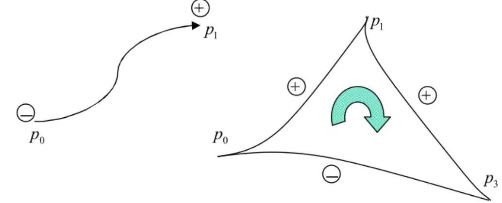
q=(p₀p₁…p_q) have an induced orientation given by

(-1)i( p₀…p_i₁pi1…pq), for i = 0, …, q .

The boundary of a q-simplex is the sum of all its (q-1)-dimensional faces, taken with the induced orientation:

q



( p₀… p_q)=

1

q

i



(-1)i( p₀…p_i1p_i1…p_q). Here are some examples, see fig.3.

A one-simplex



1= (p₀p₁) is given by its two vertices. Its boundary is



(p₀p₁) = p₁- p₀.

The boundary of a two-simplex



2( p₀p₁p₂) is what you get by going around the triangle in the order p₀



p₁



p₂



p₀:



( p₀p₁p₂) = ( p₀p₁) - ( p₀p₂) + (p₁p₂) = ( p₀p₁) + (p₁p₂) + (p₂p₀). The boundary of a zero-simplex is 0.

Fig. 3 - Faces of simplexes with the induced orientation

4. Cellular spaces

Another way to calculate homology groups is cellular decomposition of the object. Cellular space (or CW-complex, which is the same) is Hausdorff topological space, represented as a union of non-intersecting sets (called cells)

X=

(

)

q

q i q J i I

e

 

 

where q is a dimension of a cell

e

_iq ; i is its number;

I

_q is some set, corresponding to dimension q ; J is a subset of the set of integer non-negative numbers.

In addition, the following conditions must be satisfied:

1. Each cell of zero dimension is a point of X. For every positive q the closure

e

_iq of each cell

e

_iq is the image of a closed q – dimensional ball

B

q under some continuous map (called characteristic map)

:

q q

i

B





q i

e

,

where

e

_iq



X , and the restriction of this map to the open ball

int

B

q is a homeomorphism. Here ball

B

q is an ordinary ball in q– dimensional Euclidian space Rq:

0

p

1

p







_

0

p

1

p

q

B

= {

w



1;

w



Rq}

2. (C-axiom – “closure finite”).

A boundary of each cell (with dimension more or equal than 1) is contained in a union of a finite number of cells of fewer dimensions. 3. (W-axiom – “weak topology”).

A subset

K

of X is closed if and only if the intersection

K



e

_iq is closed for every cell

e

_iq of space X.

It is easy to understand that for finite CW-complexes (i.e. consisting of finite number of cells) C-axiom and W-axiom are held automatically.

Consider an important example of a cellular subspace of X – its skeleton

p

sk

X =

,

q J q p





( q

i



I

q i

e

) ,

where p is an integer non-negative number.

Thus, from the above definitions we can obtain the next procedure of cellular spaces constructing. Consider a restriction

F

_iq of the characteristic map



_iq to the boundary

S

_iq1 of the closed q-dimensional ball

B

_iq, and after that consider continuous map from a union of spheres into a skeleton:

q

F

:

q

i



I

1

q i

S





sk

_q₁X ,

so that

F

_iq is a restriction of

F

q to the sphere

S

_iq1. Thus,

q

sk

X =

sk

_q1X



_Fq ( q

i



I

q i

B

)

Continuous map

F

q is called gluing map (or attaching map). Indeed, gluing map identifies each point x from

S

_iq1 with its image

q

F

(x)



sk

_q1X . So, we have a sequence

0

sk

X



sk

₁X



…



sk

_qX



…



X , which is called a filtration.

Roughly speaking, if we add a differential structure to a cellular space, we will obtain a smooth manifold. Differential geometry, an important branch of mathematics, describes various properties of manifolds Two-dimensional smooth manifold is called a surface. Fig.4 depicts the interaction among various spaces.

Fig. 4

In [19-22] so-called homotopy model based on Morse theory for smooth manifolds was constructed. The scheme

VRML data



Homotopy data



VRML data

is used there. Homotopy data consist of information about critical points of Morse function chosen as a height function (Reeb graph, see fig.5), cross sections, and other. Each critical point of Morse function [1] has its index (an integer non-negative number). For example, for peak points index



=2, for saddle points



=1, and for pit points



=0. Generalization of Reeb graph was used in [18] for shape recognition of geometrical objects.

Fig. 5 - Reeb graph for torus peak

saddle point

saddle point

Consider a simple example – a torus

T

2 and a cellular decomposition of it. A torus is a smooth compact orientable 2-dimensional manifold with genus g = 1 (see fig.6).

Fig. 6 - Cellular decomposition of torus

One can easily distinguish two main circles: along and across a torus. On fig.6 they are intersecting at a point A. Indeed, torus is a direct product of these two circles

2

T

=

S

1



S

1.

Thus we are able to consider the following cellular decomposition: one 0-cell

e

o(that is a point A ); two 1-cells

e

₁1 and

e

1₂– open intervals (that are main circles without point A ); and one 2-cell

e

2– an open rectangle. As for skeletons, we have:

0

sk

_T

2₌

_e

o _{is simply the point A;}

1

sk

_T

2

=

e

o+

e

₁1+

e

1₂ is a bouquet S1∨S1 of two circles;

2

sk

_T

2₌

_e

o₊ 1 1

e

+

e

1₂+

e

2 is the torus

T

2 itself. As for characteristic and gluing maps, in this example we have:

1 1



:

B

₁1



e

₁1,



1₂:

B

₂1



e

₂1

1 1

F

:

S

₁0



e

0,

F

₂1:

S

₂0



e

0,

where

S

₁0,

S

₂0, are couples of points by definition,

B

₁1,

B

₂1 are closed line segments. And

1

sk

_T

2 ₌ 0

sk

_T

2

1

F



(

2

1

i

i







1

i

B

) = S1∨ S1. Indeed, the next general statement is held.

Theorem 2. A closed orientable surface M2 with genus g has a cell decomposition M2=

e

o+ (

a

₁+

b

₁+…

a

_g+

b

_g) +

e

2,

where

e

o is a point on M2, and

a

_i,

b

_i are loops starting and ending at

e

o.

There is a close connection between cell decomposition and triangulation of a surface. Triangulation is a decomposition of a surface into a set of triangles in some reasonable way (i.e. in the way of simplicial decompositions, see [1]).

Theorem 3. Any smooth compact 2-dimensional manifold admits a triangulation.

The integer number E(M) =

( 1)

j

j

indP

P C





, where

P

_j are critical points of Morse function,

indP

_j are their indexes, C is the set of critical points of this Morse function, is called Euler characteristic of a given manifold M.

Theorem 4. For a triangulation of a surface E (M) = V –E +F = 2–2g,

where V is a number of vertices, E is a number of edges, F is a number of faces, and g is a genus of the surface M.

We can define the notion of homology groups for cellular space in the way, similar to one for simplicial complexes. The (cell) boundary operator is a homomorphism

q



: C_q(X)



C_q1(X) ,



eq=



[ eq:e_iq1] eq_i1,

where the sum is over all (q-1)-cells of X, and the integer indexes [ eq:eq_i1] are introduced by degree of a map (e.g., see [1]). Like its simplicial counterpart, the cell boundary operator satisfies

q





_q1= 0 for all q.

A q-chain is called a q-cycle if its boundary is 0. It is a q-boundary if it is a boundary of some (q+1)-chain. Thus, the group of q-cycles is

Z_q(X) = ker



_q ,

And the group of q-boundaries is B_q(X) = im



_q₁ .

The q-th cell homology group is the quotient H_q(X)= Z_q(X)/ B_q(X) .

Theorem 5. If a topological space has two distinct cell decompositions, the cell homology groups are the same for both decompositions. The polyhedron K of a simplicial complex is a cell space, in an obvious way (fix a homeomorhism between a closed ball and a standard closed simplex in dimension k). Consequently, for any such K we can calculate its simplicial homology group and the cell homology group.

Theorem 6. If X is the polyhedron of a finite simplicial complex, the simplicial homology groups and the cell homology groups of X are isomorphic.

Thus, we know two ways of computing homology groups: if we have a cell decomposition, we can compute the cell homology, and if we have a simplicial structure, we can compute the simplicial homology. The result is the same. If the numbers [ eq:eq_i1] are known, it is not difficult (easier, than in the case of simplicial complexes) to calculate cell homology groups, using the technique of homology exact pair sequence [1,2].

There are many profound theorems on cellular spaces. We just want to mention some of them. Theorem 7. Given two homotopically equivalent gluing maps

F

q and

G

q

q

F

,

G

q: q

i



I

1

q i

S





sk

_q₁X,

then spaces

sk

_q1X



_Fq ( q

i



I

q i

B

) and

sk

_q1X



_Gq ( q

i



I

q i

B

) are homotopically equivalent.

Theorem 8. Let f be a Morse function on a compact smooth manifold M. Then M is homotopically equivalent to a finite CW-complex containing one cell of dimension



for each critical point of f of index



.

Continuous map f : X



Y, where X and Y are cellular spaces, is called a cellular map, if f (

sk

_qX )



sk

_qY

for each integer non-negative q.

Theorem 9 (about cellular approximation). If X and Y are cellular spaces and f is a continuous map f : X



Y

than cellular map g exists: g : X



Y

that f and g are homotopically equivalent maps.

References

1. A. T. Fomenko, T. L. Kunii “Topological Modeling for Visualization”, Springer, 1998 2. A. T. Fomenko, D. B. Fuchs “Course of Homotopic Topology.” Kluwer Academic Publishers

3. Paoluzzi A. et al. Dimension-independent modeling with simplicial complexes. ACM Transactions on graphics 12, 1 (January 1993), 56-102

4. Bertolotto M. et al. Pyramidal simplicial complexes. In Solid Modeling’95, pp.153-162

5. Lang V., Lienhardt P. Geometric modeling with simplicial sets. In Pasific Graphics’95, pp.475-493

6. Weiler K. The radial edge structure: a topological representation for non-manifold geometric boundary modeling. In Geometric modeling for CAD applications. Elsevier Science Publish., 1988

7. Brisson E. Representation of d-dimentional geometric objects. PhD thesis, U. of Washington, 1990

8. T. L. Kunii “Valid Computational Shape Modeling: Design and Implementation.” World Scientific, December 1999 9. T. L. Kunii “Homotopy Modeling as World Modeling.” Proceedings of Computer Graphics International ’99, pp.130-141. 10. T. L. Kunii “Technological Impact of Modern Abstract Mathematics” Proceedings of Third Asian Technology Conference in Mathematics, 1998, pp.13-23.

11. T. L. Kunii, Y. Saito, M. Shiine “A Graphics Compiler for a 3-Dimensional Captured Image Database and Captured Image Reusability.” Proceedings of CAPTECH’98.

12. T. L. Kunii “Graphics with Shape Property Inheritance.” Proceedings of Pacific Graphics’98.

13. T. L. Kunii “The 3-rd Industrial Revolution through Integrated Intelligent Processing Systems.” Proceedings of IEEE First International Conference ICIPS’97, pp.1-6

14. K. Ohmori, T.L.Kunii “Shape Modeling Using Homotopy”, IEEE 2001. 15. J. Popovic, H.Hoppe. Progressive Simplicial Complexes. SIGGRAPH’1997

16. M.Muller-Hanneman. Hexahedral mesh generation by successive dual cycle elimination. Engineering with computers 15 (1999), pp. 269-279

17. T. Ngo et al. Accessible animation and customizable graphics via simplicial configuration modeling. SIGGRAPH’2000