Representing hydrodynamically-important blocking features in coastal or riverine lidar topography

(1)

NHESSD

3, 1427–1452, 2015

Representing hydrodynamic features from lidar

topography

B. R. Hodges

Title Page

Abstract Introduction

Conclusions References

Tables Figures

◭ ◮

Back Close

Full Screen / Esc

Printer-friendly Version Interactive Discussion

Discussion

P

a

per

|

Discussion

P

a

per

|

Discussion

P

a

per

|

Discussion

P

a

per

|

Nat. Hazards Earth Syst. Sci. Discuss., 3, 1427–1452, 2015 www.nat-hazards-earth-syst-sci-discuss.net/3/1427/2015/ doi:10.5194/nhessd-3-1427-2015

This discussion paper is/has been under review for the journal Natural Hazards and Earth System Sciences (NHESS). Please refer to the corresponding final paper in NHESS if available.

Representing

hydrodynamically-important blocking

features in coastal or riverine lidar

topography

B. R. Hodges

Department of Civil, Architectural, and Environmental Engineering, The University of Texas at Austin, Austin, Texas, USA

Received: 1 December 2014 – Accepted: 2 February 2015 – Published: 13 February 2015

Correspondence to: B. R. Hodges (hodges@utexas.edu)

(2)

NHESSD

3, 1427–1452, 2015

topography

B. R. Hodges

Title Page

Tables Figures

◭ ◮

Back Close

Full Screen / Esc

Discussion

P

a

per

|

Discussion

P

a

per

|

Discussion

P

a

per

|

Discussion

P

a

per

Abstract

New automated methods are developed for identifying narrow landscape features that cause hydrodynamic blocking and might have critical impacts for management models of river flooding, coastal inundation, climate change, or extreme event analysis. Lidar data processed into a fine-resolution raster (1 m×1 m) can resolve narrow blocking

fea-5

tures in topography, but typically cannot be directly used for hydrodynamic modeling. For practical applications such data are abstracted to larger scales, which can result in a loss of hydrodynamic blocking effects. The traditional approach to resolving hydro-dynamic blocking features is to represent them as cell boundaries within customized unstructured grid that is tuned to the spatial features. A new automated edge-blocking

10

approach is developed, which allows application of an arbitrary structured (Cartesian) mesh at coarser scales and provides contiguous representation of blocking features along Cartesian cell boundaries. This approach distorts the shape of a blocking fea-ture (i.e., making it rectilinear along grid cell faces), but retains its critical hydrodynamic blocking height characteristics and spatial continuity within the topographic model.

15

1 Introduction

Hydrodynamic models are useful tools for exploring how climate change, rising sea levels, and hydrological regime alterations might affect the interaction between tides, rivers and coastlines (Purvis et al., 2008; Bhuiyan and Dutta, 2012; Nardin and Ed-monds, 2014), as well as urban coastal flooding (Gallien et al., 2013; Webster et al.,

20

2014). Similarly, such models are vital in analysis of river hydrodynamics and flood-plain inundation that might be affected by changing climate patterns (Wen et al., 2013; Vastila et al., 2010). Unfortunately, modeling annual to decadal timescales for manage-ment and climate change analyses typically requires hydrodynamic model grid scales that might not adequately represent narrow blocking features. Herein we develop new

(3)

NHESSD

3, 1427–1452, 2015

topography

B. R. Hodges

Title Page

Tables Figures

◭ ◮

Back Close

Full Screen / Esc

Discussion

P

a

per

|

Discussion

P

a

per

|

Discussion

P

a

per

|

Discussion

P

a

per

|

methods for upscaling a digital elevation model of topography to ensure hydrodynamic blocking features are retained.

The working hypothesis of this paper is that at any sufficiently coarse grid scale (∆C) there might be topographic features of width scaleℓW<∆Cand length scaleℓL≥∆C that can be represented as “edge” or “face” features of the grid cell. These features,

5

if given the correct continuity across multiple grid cells, can represent hydrodynamic blocking that is lost when subgrid features are represented as topographic roughness. We will call this anedge blockingtechnique.

By way of background, the present state-of-the-art for processed lidar data can

readily provide ∼1 m×1 m topography for use in high-resolution hydrodynamic

mod-10

eling (Schubert et al., 2008; Sampson et al., 2012). Unfortunately, modeling at such fine spatial resolution invariably drives the model time step down to one second or

lower, depending on the numerical model scheme1. At such scales, even a small river

delta of 1000 ha will require ∼107 grid cells and ∼107 time steps per year of

simu-lation – pushing even a small system into supercomputer territory for multi-decadal

15

and/or Monte Carlo simulations for sensitivity analyses, which are desirable for

adap-tive coastal management. However, by coarsening to a 20 m×20 m grid resolution,

1000 hectares requires only 2.5×104grid cells and can typically be run at time steps of 10 to 30 s in a semi-implicit model2, i.e., ∼106 time steps per year of simulation. The reduced memory requirement allows multiple model instances to be

simultane-20

ously run on a standard multi-core desktop workstation. The larger allowable time step allows faster simulations over longer timescales without requiring extensive high-end computational resources. Indeed, it is likely that as computers get more powerful, our desire to decrease grid resolution will be countered by our desire to run larger areas and longer timescale simulations. Thus, the need for grid coarsening of lidar data for

25

1

The BreZo code of Sanders et al. (2010) required time steps of 0.05 s for 0.8 m triangular mesh in Schubert et al. (2008).

2

(4)

NHESSD

3, 1427–1452, 2015

topography

B. R. Hodges

Title Page

Tables Figures

◭ ◮

Back Close

Full Screen / Esc

Discussion

P

a

per

|

Discussion

P

a

per

|

Discussion

P

a

per

|

Discussion

P

a

per

hydrodynamics is unlikely to disappear, and the challenge we face is in upscaling the

topography while capturing the hydrodynamic effects of unresolved features.

As an alternative to grid coarsening, grid nesting (from fine to coarse grids) can be applied to somewhat reduce computational costs (e.g., Webster et al., 2014), but such methods inherently require an expert modeler to make a judgement as to where model

5

resolution might be coarsened. Artificial porosity approaches seem appropriate for ur-ban areas with multiple pathways around unresolved objects (Sanders et al., 2008), but it is not clear that they are necessarily useful in broader natural settings or where narrow objects are blocking over multiple cells. Quadtree subgrid nesting for

hydro-dynamic models appears to be one approach for upscaling effects of fine-resolution

10

topography without resorting to edge features (Stelling, 2012; Volp et al., 2013), but such methods are still in the early stages of development and cannot be considered a definitive solution. Indeed, it is not clear that simple application of quadtree methods would necessarily preserve contiguous blocking edges, so combining quadtree with the present edge blocking technique might be necessary.

15

Upscaling of lidar data presents hydrodynamic modeling challenges (Fewtrell et al., 2008). Prior to lidar, our topographic data was generally coarser than model grid scales (Bates, 2004), so translating topography to a model grid was a matter of simple interpo-lation from a sparse data set and calibrating roughness for effects of unknown features. With the advent of lidar, as noted by Bates et al. (2003) “we need methods to identify

20

and connect linear topographic features . . . given their significant hydraulic impact.” Despite more than 75 citations of this pioneering work, the challenge ofidentifying and connecting linear topographic features has not been addressed in the past decade, and thus provides the fundamental motivation for the present work. Herein we present a new method for identifying, extracting, and representing topographic features that

ex-25

tend over multiple coarse-grid cells, but are so narrow that their hydrodynamic blocking

effects would be lost in common upscaling techniques.

(5)

NHESSD

3, 1427–1452, 2015

topography

B. R. Hodges

Title Page

Tables Figures

◭ ◮

Back Close

Full Screen / Esc

Discussion

P

a

per

|

Discussion

P

a

per

|

Discussion

P

a

per

|

Discussion

P

a

per

|

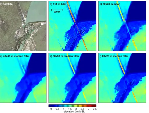
across the Nueces River delta in Texas, USA, just outside the City of Corpus Christi. The dike is approximately 5 m across at the top and 15 m across at the base. If the lidar data is rasterized a to 20 m×20 m grid using a simple arithmetic mean of the finer scale data (Fig. 1c), the dike loses both its overall blocking height and continuity. A hydrody-namic model using this coarser grid would have flow paths through the dike at 1.5 to

5

2 m a.s.l. rather than being contiguously blocked at a 3 m elevation.

Where dikes, embankments, and complex topography are narrower than a practical hydrodynamic grid, the traditional solution has been use of unstructured grids designed with cell boundaries coincident to narrow blocking features (e.g., Cobby et al., 2003; Tsubaki and Fujita, 2010). Unfortunately, unstructured grids usually require significant

10

expertise and “hands-on” artistry to develop an acceptable balance between hydro-dynamic modeling practicality and fidelity to the physical topography (Schubert et al., 2008; Mandlburger et al., 2009). As another approach, Ryan and Hodges (2011) mod-eled the 7500 hectares of the Nueces River delta with a structured Cartesian grid where the narrow railroad dike across the delta (Fig. 1) was represented as an elevated edge

15

feature in a 2-D hydrodynamic model. Identifying this contiguous edge feature on the raster grid was a labor-intensive manual task, but was critical to obtaining the correct hydraulic blocking effects.

It can be stated without reservation that hydrodynamic modeling is simpler if a single size and shape of grid element is used across an entire domain. Such a grid might be

20

called an “arbitrary” grid as, by definition, it is not tuned to match any particular topo-graphic feature. The problem with arbitrary grids is that at coarse resolution they will not have the proper connectivity of either narrow flow paths or narrow blocking structures. Thus, the simplicity of arbitrary gridding does not necessarily imply a better model. However, if narrow blocking features can be upscaled to the edges of the arbitrary grid

25

(6)

NHESSD

3, 1427–1452, 2015

topography

B. R. Hodges

Title Page

Tables Figures

◭ ◮

Back Close

Full Screen / Esc

Discussion

P

a

per

|

Discussion

P

a

per

|

Discussion

P

a

per

|

Discussion

P

a

per

For an arbitrary gridding approach to actually simplify modeling, the definition of the coarse-grid edge blocking must be automatic – else we are back to treating grid defini-tion as a labor-intensive art form. This paper introduces a “hands-off” topographic fea-ture extraction system that provides automated identification and representation of fine-scale topographic features that are hydrodynamically important blockages at coarser

5

scales. This new approach captures both the obvious large-scale features (such as the railroad dike) as well as smaller features that are more difficult to identify but might have hydrodynamic blocking influences that are lost in traditional upscaling algorithms. The new approach uses Cartesian grids that are relatively easy to create, modify, and hydrodynamically model. Although unstructured grids have been popular over the past

10

two decades as a way to direct computational power at specifically desired scales, one can make the argument that continually increasing computer power will eventually lead to a return to structured grid modeling that provides simpler automation, requires less expertise in model development, and easier communication between models. It should be noted that this edge blocking concept could also be applied to an arbitrary

unstruc-15

tured grid, however, the object identification and parsing techniques herein rely heavily on the Cartesian structure of the coarse grid to provide simple algorithms.

This paper provides a set of methods to represent fine-scale topographic data in

a manner that allows effective hydrodynamic modeling of blocking features at coarser

scales on a Cartesian grid. Full implementation and testing of these ideas requires

20

a hydrodynamic model that discriminates between elevations of the grid cell center and elevations of the grid cell faces, which is typically not difficult to include (e.g., Casulli and Cheng, 1992). However, the impact of these new face blocking techniques on the hydrodynamic solution is a subject for future investigations, and will not be addressed herein.

(7)

NHESSD

3, 1427–1452, 2015

topography

B. R. Hodges

Title Page

Tables Figures

◭ ◮

Back Close

Full Screen / Esc

Discussion

P

a

per

|

Discussion

P

a

per

|

Discussion

P

a

per

|

Discussion

P

a

per

|

2 Methods

The goal of our lidar processing is to produce a coarse Cartesian grid at some scale

∆C >∆F that retains valuable hydrodynamic characteristics associated with contigu-ous blockage features (e.g., the railroad dike in Fig. 1). In a conventional Cartesian raster grid, each cell has a single piece of data: the landscape elevation. However, for

5

the coarse grid we will store a representative value for the elevation over the bulk of the grid cell and separate blocking elevation values on each cell face. For convenience in data processing, we will limit our focus to systems where the coarse-to-fine raster ratio R_∆= ∆C/∆F is an integer. For sufficiently fine resolution lidar data, this is not a significant limitation. It follows that the coarse-grid raster is of sizencx×ncy, where

10

ncx=nfx/R∆ andncy=nfx/R∆, with nfxandnfy as the number of fine-grid cells in the

data set (this generally requires truncating some fine-grid data at edges to ensure in-tegral values forn’s). For simplicity in exposition, we will confine ourselves to the case

where thex and y directions are resolved with the same R_∆, although the method is

readily extensible to rectangular vice square grid cells.

15

The general procedure for data processing is:

1. create a fine-grid background topography (Fig. 1d);

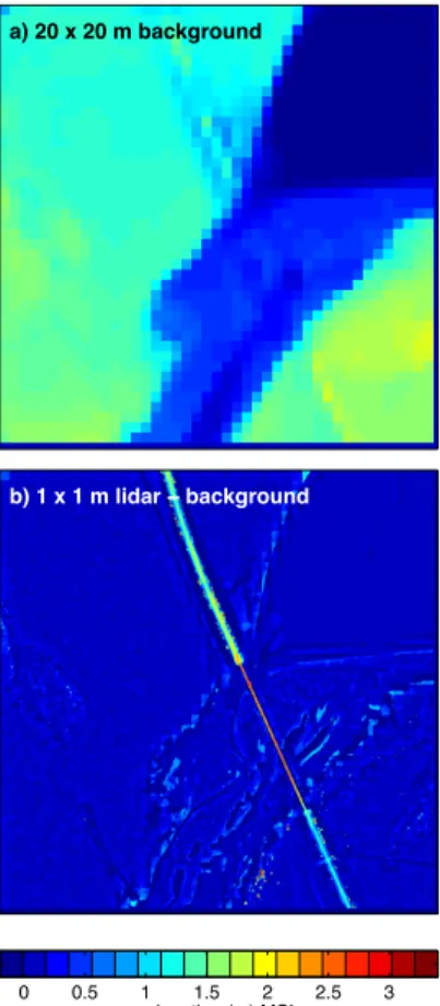
2. create a coarse-grid representation of background topography (Fig. 2a);

3. compute the difference between fine and coarse topography (Fig. 2b);

4. identify contiguous objects that occur in the difference set (Fig. 3);

20

5. identify blocking objects and assign elevations to grid cell faces (Fig. 4).

2.1 Fine-scale background topography

The first step is to separate unresolvable topographic features (at coarse scale ∆C)

(8)

NHESSD

3, 1427–1452, 2015

topography

B. R. Hodges

Title Page

Tables Figures

◭ ◮

Back Close

Full Screen / Esc

Discussion

P

a

per

|

Discussion

P

a

per

|

Discussion

P

a

per

|

Discussion

P

a

per

look like with coarse-scale unresolvable features removed. Herein we apply a

me-dian filter, which was originally designed for image noise removal but has proven more widely useful, e.g., removing the signature of large woody debris from bathymetric data (White and Hodges, 2005). A median filter replaces the value at position (x,y) with the median of the values in some neighborhood around the point; the neighborhood size

5

is defined as the filter size. The filter operation is accomplished on a moving window over the fine-scale grid to produce a smooth rendition of the background elevations that are resolvable at a coarser resolution; that is, the original resolution of the data set is maintained (e.g., unlike the averaging in Fig. 1c) while the unresolvable features are

removed. For example, the 1 m×1 m lidar data is processed with different size median

10

filters as shown in Fig. 1d–f, providing smooth, high-resolution background elevations. Clearly, the filter scale for defining background topography should be equal to or greater than the desired coarse-grid scale. If the median filter is smaller than the coarse grid, then objects that cannot be resolved will remain in the filtered data set, and hence not in the difference data set (see below). Indeed, it seems prudent to generally apply

15

a median filter that is twice the desired coarse-grid scale to ensure that the data set is su_fficiently smooth for hydrodynamic modeling. That is, if a 20 m×20 m coarse grid is desired and a 20 m×20 m median filter is applied, there can be features slightly larger than 20 m that will appear across two coarse grid cells and hence will not really be hydrodynamically resolved. This e_ffect is clear in Fig. 1f, where the 20 m×20 m filter

20

shows a partial signature of the railroad dike that would be lost in upscaling to the coarse grid as in Fig. 1c.

2.2 Coarse background and difference data set

The median filtered fine-scale data, Fig. 1d, is used to produce a coarse-grid approxi-mation of the landscape elevation, Fig. 2a. This step can be accomplished using either

25

(9)

NHESSD

3, 1427–1452, 2015

topography

B. R. Hodges

Title Page

Tables Figures

◭ ◮

Back Close

Full Screen / Esc

Discussion

P

a

per

|

Discussion

P

a

per

|

Discussion

P

a

per

|

Discussion

P

a

per

|

(i.e., using identical values for all the fine cells within a single coarse-grid cell) so that a fine-scale difference map can be created (Fig. 2b).

2.3 Identification of objects

The difference map contains both negative objects (unresolved depressions) and

posi-tive objects (unresolved blockages). The present work focusses on the posiposi-tive objects3

5

that are relatively easy to handle in a hydrodynamic model that includes cell edge el-evations. To identify blocking positive objects, a cutoffheight (∆h) is specified above which an object is deemed a hydrodynamic blockage rather than simply topographic

roughness. The number and size of objects will be a function of this cutoff. For the

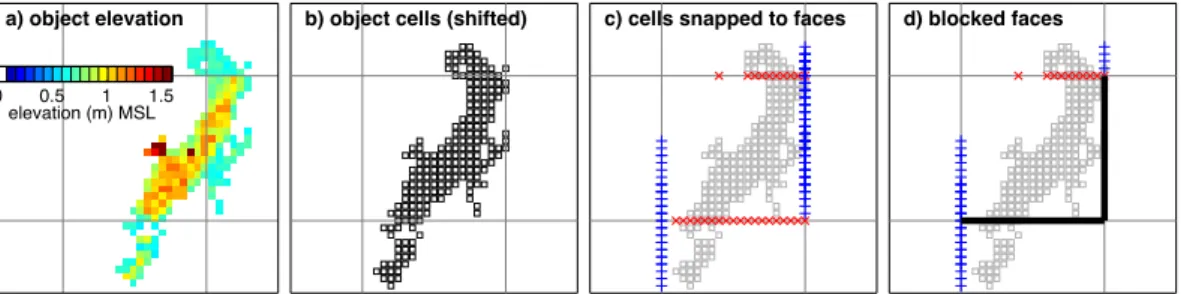
present demonstration, the cutoffheight is ∆h=0.2 m. A binary data set can be

de-10

fined as {0,1} based on whether fine-grid cells are respectively below or above ∆h ,

as shown in Fig. 3a. The binary data can be manipulated using bwmorph and

bw-boundariesin the Matlab Image Processing Toolbox. The bwmorphfunction, through its “clean” option, identifies isolated pixels in a binary image and removes them – an

image noise removal operation. Thebwboundariesfunction uses the Moore-Neighbor

15

tracing algorithm (Gonzalez et al., 2004) to identify individual objects that are formed by contiguous pixels and unconnected to other objects, as shown in Fig. 3b. Herein,

the “noholes” option ofbwboundariesis used to remove any depressions in the center

of objects.

For the present work, it is also useful to remove objects that are too small to block

20

a coarse grid cell; i.e., for a 20 m×20 m coarse grid based on a 1 m×1 m data set

(R_∆=20), any object in Fig. 3a that consists of less thanNc=20 fine-grid cells cannot hydraulically block a coarse-grid cell, and can be excised from the object data set. To allow some flexibility, it is useful to define the removal criterion asNc≤R∆−δ, where

3

(10)

NHESSD

3, 1427–1452, 2015

topography

B. R. Hodges

Title Page

Tables Figures

◭ ◮

Back Close

Full Screen / Esc

Discussion

P

a

per

|

Discussion

P

a

per

|

Discussion

P

a

per

|

Discussion

P

a

per

δ∈ {0, 1, 2,. . .}is a user-defined parameter that allows nearly blocking objects (δ >0) to be retained in the object data set. Hereinδ=1 is used.

2.4 Snap-grid object blocking

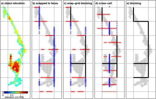
Each object can be processed separately to provide hydraulic blocking conditions on both row and column faces of a coarse grid cell. A typical object and its elevations

5

(Fig. 4a) has a binary representation at the fine-grid level, as shown in Fig. 4b. Let

fo(xc,yc) be the set of fine-grid cells of the object, where xc and yc are coordinates measured relative to the coarse grid. The coarse grid demarcation lines are, by defini-tion, integer values in our coarse-grid numbering scheme. This is perhaps slightly un-conventional for hydrodynamic modelers as the coarse-grid cell centers are therefore

10

at non-integer values, i.e., the location (xc,yc)=(i−1/2,j−1/2) defines a coarse-grid cell in the raster set fori={1, 2, 3,. . .ncx},j=

1, 2, 3,. . .ncy with faces at coarse-grid

indexes (xc,yc)∈

(i,j−1/2), (i−1,j−1/2), (i−1/2,j), (i−1/2,j−1) . Using this in-dexing, we can defineGy(i−1/2,j)=fo(xc, round(yc)) as a set of fine-grid cells of vary-ingxc that are “snapped” to an integerycface (the red×markers in Fig. 4c). Similarly

15

Gx(i,j−1/2)=fo(round(xc),yc) is the set of blocking cells of varying yc snapped to

an integer xc face, (the blue +markers in Fig. 4c). For the purposes of determining

whether or not blocking occurs, the cells setsG_x and G_y are true mathematical sets

that do not include duplicate values. However, data sets with duplicates (denoted as

Gyy andGxx) are retained for computation of blocking height (discussed below).

20

To determinesnap-grid blockingof coarse grid faces (Fig. 4d), the sizes of setG_y(i−

1/2,j) andG_x(i,j−1/2) are defined asN_y(i−1/2,j) and N_x(i,j−1/2), respectively.

These are the number of unique values ofxc on a round(yc) face (red ×markers on

a column face) and the number of uniqueycvalues on a round(xc) face (blue+markers on a row face). Snap-grid blocking occurs along coarse-grid column faces that satisfy

25

(11)

NHESSD

3, 1427–1452, 2015

topography

B. R. Hodges

Title Page

Tables Figures

◭ ◮

Back Close

Full Screen / Esc

Discussion

P

a

per

|

Discussion

P

a

per

|

Discussion

P

a

per

|

Discussion

P

a

per

|

and coarse-grid row faces that satisfy

N_x(i,j−1/2)≥R_∆−δ (2)

where δ is the same δ∈ {0, 1, 2,. . .} used for identifying objects (above). Note that

this approach allows the fine cells to serve both as blocking in thex andy directions

simultaneously, which is necessary to represent the hydraulic blocking of objects at

5

an angle to the coarse grid. After a face is blocked, e.g., as shown in Fig. 4d, the correspondingGy(i−1/2,j) andGx(i,j−1/2) are set to zero so that fine-grid cells used

to define a snap-grid block are not used in computing cross-cell blocking (discussed

below).

2.5 Small object shift

10

The snap-grid blocking approach will necessarily depend on the spatial relationship between the objects and the coarse grid. For small objects, a slight shift of the object position can change whether or not the object is judged to be blocking. For example, the lower column face blocking Fig. 4d would not have been identified as blocking in the original object position, shown in Fig. 4a, because some of the fine-grid cells

15

would have shown up in an adjacent column such that Eq. (1) would not have been satisfied for either face. For small objects (less than 1.5_∆C), it is convenient to simply shift the object (as in Fig. 4b) to maximize the number of fine-grid blocking cells within a single coarse grid cell. As long as the shift is less than∆C/4, it does not significantly affect the coarse-grid physical relationships. Object shifting can be accomplished with

20

an automated algorithm that is based on the total extent of a small object and the overhang of the object into adjacent cells.

2.6 Cross-cell object blocking

Depending on an object’s topology, the blocked faces determined by the snap-grid approach (described above) might not provide a contiguous blocked path. Consider

(12)

NHESSD

3, 1427–1452, 2015

topography

B. R. Hodges

Title Page

Tables Figures

◭ ◮

Back Close

Full Screen / Esc

Discussion

P

a

per

|

Discussion

P

a

per

|

Discussion

P

a

per

|

Discussion

P

a

per

the larger object in Fig. 5a, where snap-grid blocking provides the results in Fig. 5b

and c. It is clear that some hydraulic blocking has not been captured: theG_x (the blue

+ markers) and Gy (red × markers) in the second coarse-grid cell from the top do

not satisfy Eqs. (1) or (2) as they are split between different faces. Furthermore in the lowermost coarse-grid cell, the red×markers on either face are insufficient for blocking.

5

These effects arise because the snap-grid approach uses rounding, which can split the

blocking fine-grid cells to the upper and lower faces of the coarse grid cell. To address

this issue, we define across-cell blockingapproach for column and row faces.

Cross-cell blocking is conducted after snap-grid blocking and only uses the fine-grid Cross-cells that

were notapplied in snap-grid blocking; e.g., the remaining red×and blue+in Fig. 5c.

10

For the coarse-grid cell centered at (i−1/2,j−1/2), we define sets of unique fine-grid blocking cells across the cell center as

Hy(i−1/2,j−1/2)=Gy(i−1/2,j) ∪ Gy(i−1/2,j−1) (3) H_x(i−1/2,j−1/2)=G_x(i,j−1/2) ∪ G_x(i−1,j−1/2) (4)

which are illustrated in Fig. 5d. Blocking conditions are defined similar to Eqs. (1) and

15

(2), usingNy and Nx as the size of the unique Hy and Hx cell sets. For determining

object blocking height (discussed below), we also define sets that retain non-unique elements,

H_yy(i−1/2,j−1/2)=G_yy(i−1/2,j) ∪ G_yy(i−1/2,j−1) (5)

Hxx(i−1/2,j−1/2)=Gxx(i,j−1/2) ∪ Gxx(i−1,j−1/2). (6)

20

As theHy andHx fine-cell sets cross the coarse-cell center, face blocking could be

at either of the grid cell faces, as shown by dashed blocking lines in Fig. 5d. Indeed, there can be more than one set of blocking faces that provides a reasonable repre-sentation of cross-cell blocking. The critical issue is ensuring that cross-cell blocking is contiguous; i.e., there are choices for cross-cell blocking faces in Fig. 5d that would

25

(13)

NHESSD

3, 1427–1452, 2015

topography

B. R. Hodges

Title Page

Tables Figures

◭ ◮

Back Close

Full Screen / Esc

Discussion

P

a

per

|

Discussion

P

a

per

|

Discussion

P

a

per

|

Discussion

P

a

per

|

only a single blocked end point (e.g., the lowermost complete cell in Fig. 5d), then the cross-cell blocked face (either row or column) must connect to that blocked end. If a coarse cell contains two blocked end points, then the algorithm must distinguish be-tween diagonally-blocked points (e.g., the 2nd coarse cell from the top in Fig. 5d) and co-linear blocked end points along a face (either row or column). Where two blocked

5

end points are along a single column face and cell-center blocking for a column face exists (red◦), the cell-center blocking logically must be along the face that connects the blocked end points. Similarly, where two blocked end points are along a row face and cell-center blocking for a row face is indicated (blue△), then the blocking is necessarily along the row face connecting the blocked end points. However, where two blocked end

10

points are co-linear along a column face and the cell-centered blocking is indicated for a row face (or vice versa), then the choice of which face to block may be taken arbitrar-ily. Similarly, when two blocked end points are diagonally opposed, the selection of the blocking face is arbitrary. Note that these arbitrary choices will necessarily set up a con-dition where three end points are blocked. Because rows and columns are processed

15

sequentially, diagonal blocking of two end points solved using columns (first cycle) sets up a cell with three blocked end points for solving using rows (second cycle). If three end points are blocked, then the cross-cell blocking must connect the two blocked end points that are co-linear along the column or row face (as appropriate), which ensures continuity of the feature.

20

In the present data set, all the objects achieved contiguous edge-blocking represen-tations using the snap-grid and cross-cell object blocking algorithms outlined above. However, one can imagine a feature that is longer and narrower than shown in Fig. 5 for which the procedure might fail. For a long narrow feature, it is possible that multiple iterations of the cross-cell algorithm would be required to define a blocking condition.

25

That is, the cross-cell algorithm described above combines (for example) theGx

block-ing cells of two opposite column faces into a sblock-ingle cell-centeredHx that is tested for

(14)

evalu-NHESSD

3, 1427–1452, 2015

topography

B. R. Hodges

Title Page

Tables Figures

◭ ◮

Back Close

Full Screen / Esc

Discussion

P

a

per

|

Discussion

P

a

per

|

Discussion

P

a

per

|

Discussion

P

a

per

ated on the cell face for blocking. This iterative approach can be continued forJx,Kx,

etc. until blocking is achieved or the coarse-grid length of the object is reached.

2.7 Object blocking height

The snap-grid and cross-cell blocking methods determine the faces blocked by an

ob-ject. To estimate the blocking height associated with each face we return to the Gxx,

5

Gyy,Hxx, andHyy sets that define the all the fine grid cells associated with a particular

blocked grid face. We do not attempt to determine the physical blocking height based on orientation of the fine-grid cells within the coarse-grid cell, but instead use a simple statistical analysis. If the number of fine cells inGxx (for example) is less than 2R∆then

we use the median of G_xx as the blocking height. Where the number of fine cells is

10

equal to or larger than 2R_∆, then we take the median of the largest half of the data set, i.e., the height of the 75th percentile.

3 Results and discussion

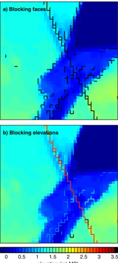
Applying theseedge-blockingmethods to the lidar data of Fig. 1b results in coarse-grid

elevations and edge blocking shown in Fig. 6. Note that many of the blocked faces are

15

relatively close to the heights of adjacent cells, and so are not obvious in Fig. 6b. The method is clearly successful in capturing the blocking of the railroad dike across the landscape, which was the primary motivation for this work. However, it should be noted that the narrow section of the railroad dike across the open water sections in Fig. 1a and b is actually a bridge, which is not hydraulically blocking and should be removed from

20

the coarse data. Removing the bridge from the lidar data at the 1 m×1 m scale before

edge blocking is applied is perhaps possible, but is difficult to automate as one must (i) identify bridge pixels and how they are different from dike pixels, and (ii) decide what fill values to use for the bridge pixels. An advantage of the edge blocking approach is that it simplifies removing the bridge from the coarse-grid data set, although we

(15)

NHESSD

3, 1427–1452, 2015

topography

B. R. Hodges

Title Page

Tables Figures

◭ ◮

Back Close

Full Screen / Esc

Discussion

P

a

per

|

Discussion

P

a

per

|

Discussion

P

a

per

|

Discussion

P

a

per

|

have not yet developed an automated approach for this task. Once the edge blocking data set is defined, as in Fig. 6b, the start and the end of the bridge section (visually apparent from the change in the width of the dike in Fig. 1b) can be used to identify the edge blocking cells in between. These data are easily removed from the edge cell set – i.e., their values are simply set to “not a number.” That is, where edge blocking

5

is not identifiable, there is no need to store any edge-blocking heights. In theory, this

technique might have wider applicability in removing the bridge from the original 1 m×

1 m lidar. It might be possible to trace back the relationship between the bridge edges removed, the pixels that represented this blocking (i.e., G_xx,G_yy, H_xx and H_yy), and

the difference data set of Fig. 2b so the corresponding bridge pixels in the 1 m×1 m

10

lidar Fig. 1b can be replaced by their median-filtered values from Fig. 1d.

Although the median filter for a large data set can be computationally expensive, the edge blocking algorithm is otherwise relatively simple and inexpensive. Raw object identification from the binary image (Fig. 3a) provides 3754 individual objects from the

7.5×105pixels; however 2075 of these are single pixel objects that are easily

elimi-15

nated. Further removing objects where Nc≤R_∆−δ leaves only 129 objects for

pro-cessing (Fig. 3b). During the propro-cessing steps, only 56 objects were found to be large enough to block any cell faces, and 21 of these blocked only a single cell face. The importance of such single-face blocking should be considered with analysis in hydro-dynamic simulations. It may be that such blocking is better represented by roughness

20

coefficients.

A potential area where the edge-blocking method might be expanded is in the esti-mation of topographic roughness, which has been a subject of extensive prior research (e.g., Abu-Aly et al., 2014; Casas et al., 2010; Dorn et al., 2014; Forzieri et al., 2011; Straatsma and Baptist, 2008). By defining edge features, a portion of the difference

be-25

tween the grid cell elevation and subgrid features can be removed from the roughness estimation; i.e., we could use (i.e.,Gxx,Gyy,Hxx andHyy) to remove pixels that have

(16)

NHESSD

3, 1427–1452, 2015

topography

B. R. Hodges

Title Page

Tables Figures

◭ ◮

Back Close

Full Screen / Esc

Discussion

P

a

per

|

Discussion

P

a

per

|

Discussion

P

a

per

|

Discussion

P

a

per

There are a number of areas in which the present method could be improved. At several places along the railroad dike there are coarse grid cells that are bounded on all sides by edge blocking. This occurs for cells that are almost directly centered on the dike such that the cross-cell blocking method results in blocked faces in all directions. Arguably, these coarse-grid cell centers should simply be filled in with the average of

5

the blocked cell faces so that they do not appear as artificial depressions. However, in marshlands there might be actual depressions surrounded by blocking topography that should not be simply filled in. Thus, the method could be improved by an algorithm that distinguishes between these two cases. As yet, we have not identified enough candidate depressions in our data set to test such an algorithm.

10

A key drawback of the present method is the potential for artificial blocking of narrow flow paths. This can occur where two adjacent objects provide blocked edges that are adjacent in the coarse-grid representation but are separated a narrow flow path in the fine-grid representation. Solution to this problem is likely to be found by addressing the key future challenge: identifying preferential flow paths that are unresolved at the

15

coarse grid scale (i.e., the negative objects resulting from unresolved depressions).

In Fig. 1a, we can clearly see a narrow stream channel on one side of the railroad dike. This channel is entirely absent in the final topography of Fig. 6. Such channels could be readily identified by using the snap-grid and cell-center blocking techniques as “path” techniques for negative objects (i.e., objects determined similar to Fig. 3a,

20

but using a negative∆hfor discrimination). However, it is not clear how such objects

could be used in present hydrodynamic models. Definition of preferential narrow flow paths that are unresolved within coarse-grid topography remains an area with no clear solution (D’Alpaos and Defina, 2007). However, there are interesting possibilities in 1-D/2-D model such as Viero et al. (2013) that might provide a good starting point. In

25

(17)

NHESSD

3, 1427–1452, 2015

topography

B. R. Hodges

Title Page

Tables Figures

◭ ◮

Back Close

Full Screen / Esc

Discussion

P

a

per

|

Discussion

P

a

per

|

Discussion

P

a

per

|

Discussion

P

a

per

|

4 Conclusions

This paper provides automated identification of hydrodynamic blocking features in fine-scale rasterized lidar topography, along with upscaling of the blockage to a coarser raster grid. These techniques could be used for modeling coastal flood inundation at the practical coarse-grid scales necessary for addressing large-scale adaptive

man-5

agement questions, while retaining the blocking effects of fine-scale features that can-not otherwise be captured.

A coarse grid developed with the newedge blockingtechnique could be immediately

applied in any number of 2-D and 3-D hydrodynamic models that permit grid cells to use different topographic elevations on different flow faces. Note that because raster

10

topographic data sets with separate face elevations have not been generally avail-able, many hydrodynamic models do not provide for separate cell-face elevation data. Nevertheless, some models could be readily adapted to using such data with minor modifications and new tools for input data manipulation.

Acknowledgements. This work was originally developed during US National Science Founda-15

tion Grant No. 710901 and has continued under NSF Grant No. CCF-1331610. Support of the Texas Water Development Board, the Coastal Bend Bays and Estuaries Program, the City of Corpus Christi, and the US Army Corps of Engineers was instrumental in the development of this project. The lidar data for the Nueces River delta was processed to the 1 m×1 m scale by J. Gibeaut, Texas A & M University – Corpus Christi.

(18)

NHESSD

3, 1427–1452, 2015

topography

B. R. Hodges

Title Page

Tables Figures

◭ ◮

Back Close

Full Screen / Esc

Discussion

P

a

per

|

Discussion

P

a

per

|

Discussion

P

a

per

|

Discussion

P

a

per

References

Abu-Aly, T. R., Pasternack, G. B., Wyrick, J. R., Barker, R., Massa, D., and Johnson, T.: E_ffects of LiDAR-derived, spatially distributed vegetation roughness on two-dimensional hydraulics in a gravel-cobble river at flows of 0.2 to 20 times bankfull, Geomorphology, 206, 468–482, doi:10.1016/j.geomorph.2013.10.017, 2014. 1441

5

Bates, P.: Remote sensing and flood inundation modelling, Hydrol. Process., 18, 2593–2597, doi:10.1002/hyp.5649, 2004. 1430

Bates, P., Marks, K., and Horritt, M.: Optimal use of high-resolution topographic data in flood inundation models, Hydrol. Process., 17, 537–557, doi:10.1002/hyp.1113, 2003. 1430 Bhuiyan, M. J. A. N., and Dutta, D.: Assessing impacts of sea level rise on river salin-10

ity in the Gorai river network, Bangladesh, Estuar. Coast. Shelf S., 96, 219–227, doi:10.1016/j.ecss.2011.11.005, 2012. 1428

Casas, A., Lane, S. N., Yu, D., and Benito, G.: A method for parameterising roughness and topographic sub-grid scale effects in hydraulic modelling from LiDAR data, Hydrol. Earth Syst. Sci., 14, 1567–1579, doi:10.5194/hess-14-1567-2010, 2010. 1441

15

Casulli, V., and Cheng, R. T.: Semiimplicit finite-di_fference methods for 3-dimensional shallow-water flow, Int. J. Numer. Meth. Fl., 15, 629–648, 1992. 1432

Cobby, D., Mason, D., Horritt, M., and Bates, P.: Two-dimensional hydraulic flood modelling using a finite-element mesh decomposed according to vegetation and topographic fea-tures derived from airborne scanning laser altimetry, Hydrol. Process., 17, 1979–2000, 20

doi:10.1002/hyp.1201, 2003. 1431

D’Alpaos, L., and Defina, A.: Mathematical modeling of tidal hydrodynamics in shallow lagoons: a review of open issues and applications to the Venice lagoon, Comput. Geosci., 33, 476– 496, doi:10.1016/j.cageo.2006.07.009, 2007. 1442

Dorn, H., Vetter, M., and Hoefle, B.: GIS-based roughness derivation for flood simulations: a 25

comparison of orthophotos, LiDAR and crowdsourced geodata, Remote Sensing, 6, 1739– 1759, doi:10.3390/rs6021739, 2014. 1441

Fewtrell, T. J., Bates, P. D., Horritt, M., and Hunter, N. M.: Evaluating the effect of scale in flood inundation modelling in urban environments, Hydrol. Process., 22, 5107–5118, doi:10.1002/hyp.7148, 2008. 1430

(19)

NHESSD

3, 1427–1452, 2015

topography

B. R. Hodges

Title Page

Tables Figures

◭ ◮

Back Close

Full Screen / Esc

Discussion

P

a

per

|

Discussion

P

a

per

|

Discussion

P

a

per

|

Discussion

P

a

per

|

Forzieri, G., Degetto, M., Righetti, M., Castelli, F., and Preti, F.: Satellite multi-spectral data for improved floodplain roughness modelling, J. Hydrol., 407, 41–57, doi:10.1016/j.jhydrol.2011.07.009, 2011. 1441

Gallien, T. W., Barnard, P. L., van Ormondt, M., Foxgrover, A. C., and Sanders, B. F.: A parcel-scale coastal flood forecasting prototype for a Southern California urbanized embayment, J. 5

Coastal Res., 29, 642–656, doi:10.2112/JCOASTRES-D-12-00114.1, 2013. 1428

Gonzalez, R. C., Woods, R. E., and Eddins, S. L.: Digital Image Processing Using MATLAB, Pearson Prentice Hall, Upper Saddle River, New Jersey, 2004. 1435

Mandlburger, G., Hauer, C., Höfle, B., Habersack, H., and Pfeifer, N.: Optimisation of LiDAR derived terrain models for river flow modelling, Hydrol. Earth Syst. Sci., 13, 1453–1466, 10

doi:10.5194/hess-13-1453-2009, 2009. 1431

Nardin, W. and Edmonds, D. A.: Optimum vegetation height and density for inorganic sedimen-tation in deltaic marshes, Nat. Geosci., 7, 722–726, doi:10.1038/NGEO2233, 2014. 1428 Purvis, M. J., Bates, P. D., and Hayes, C. M.: A probabilistic methodology to

esti-mate future coastal flood risk due to sea level rise, Coast. Eng., 55, 1062–1073, 15

doi:10.1016/j.coastaleng.2008.04.008, 2008. 1428

Ryan, A. and Hodges, B. R.: Modeling Hydrodynamic Fluxes in the Nueces River Delta, Tech. Rep., CRWR Online Report 11-07, Center for Research in Water Resources, Uni-versity of Texas at Austin, available at: http://www.crwr.utexas.edu/online.shtml (last access: 12 February 2015), 2011. 1431

20

Sampson, C. C., Fewtrell, T. J., Duncan, A., Shaad, K., Horritt, M. S., and Bates, P. D.: Use of terrestrial laser scanning data to drive decimetric resolution urban inundation models, Adv. Water Resour., 41, 1–17, doi:10.1016/j.advwatres.2012.02.010, 2012. 1429

Sanders, B. F., Schubert, J. E., and Gallegos, H. A.: Integral formulation of shallow-water equations with anisotropic porosity for urban flood modeling, J. Hydrol., 362, 19–38, 25

doi:10.1016/j.jhydrol.2008.08.009, 2008. 1430

Sanders, B. F., Schubert, J. E., and Detwiler, R. L.: ParBreZo: a parallel, unstructured grid, Godunov-type, shallow-water code for high-resolution flood inundation modeling at the re-gional scale, Adv. Water Resour., 33, 1456–1467, doi:10.1016/j.advwatres.2010.07.007, 2010. 1429

30

(20)

NHESSD

3, 1427–1452, 2015

topography

B. R. Hodges

Title Page

Tables Figures

◭ ◮

Back Close

Full Screen / Esc

Discussion

P

a

per

|

Discussion

P

a

per

|

Discussion

P

a

per

|

Discussion

P

a

per

Stelling, G. S.: Quadtree flood simulations with sub-grid digital elevations models, Water Man-agement, 165, 567–580, 2012. 1430

Straatsma, M. W. and Baptist, M. J.: Floodplain roughness parameterization using airborne laser scanning and spectral remote sensing, Remote Sens. Environ., 112, 1062–1080, doi:10.1016/j.rse.2007.07.012, 2008. 1441

5

Tsubaki, R., and Fujita, I.: Unstructured grid generation using LiDAR data for urban flood inun-dation modelling, Hydrol. Process., 24, 1404–1420, doi:10.1002/hyp.7608, 2010. 1431 Vastila, K., Kummu, M., Sangmanee, C., and Chinvanno, S.: Modelling climate change

im-pacts on the flood pulse in the Lower Mekong floodplains, J. Water Clim. Change, 1, 67–86, doi:10.2166/wcc.2010.008, 2010. 1428

10

Viero, D. P., D’Alpaos, A., Carniello, L., and Defina, A.: Mathematical modeling of flooding due to river bank failure, Adv. Water Resour., 59, 82–94, doi:10.1016/j.advwatres.2013.05.011, 2013. 1442

Volp, N. D., van Prooijen, B. C., and Stelling, G. S.: A finite volume approach for shallow water flow accounting for high-resolution bathymetry and roughness data, Water Resour. Res., 49, 15

4126–4135, 2013. 1430

Webster, T., McGuigan, K., Collins, K., and MacDonald, C.: Integrated river and coastal hy-drodynamic flood risk mapping of the LaHave River Estuary and town of Bridgewater, Nova Scotia, Canada, Water, 6, 517–546, doi:10.3390/w6030517, 2014. 1428, 1430

Wen, L., Macdonald, R., Morrison, T., Hameed, T., Saintilan, N., and Ling, J.: From hydrody-20

namic to hydrological modelling: investigating long-term hydrological regimes of key wetlands in the Macquarie Marshes, a semi-arid lowland floodplain in Australia, J. Hydrol., 500, 45–61, doi:10.1016/j.jhydrol.2013.07.015, 2013. 1428

White, L. and Hodges, B. R.: Filtering the signature of submerged large woody debris from bathymetry data, J. Hydrol., 309, 53–65, 2005. 1434

(21)

NHESSD

3, 1427–1452, 2015

topography

B. R. Hodges

Title Page

Tables Figures

◭ ◮

Back Close

Full Screen / Esc

Discussion

P

a

per

|

Discussion

P

a

per

|

Discussion

P

a

per

|

Discussion

P

a

per

|

a) satellite b) 1x1 m lidar

200 m

c) 20x20 m mean

d) 40x40 m median filter e) 30x30 m median filter f) 20x20 m median filter

elevation (m) MSL

0 0.5 1 1.5 2 2.5 3 3.5

(22)

NHESSD

3, 1427–1452, 2015

topography

B. R. Hodges

Title Page

Tables Figures

◭ ◮

Back Close

Full Screen / Esc

Discussion

P

a

per

|

Discussion

P

a

per

|

Discussion

P

a

per

|

Discussion

P

a

per

a) 20 x 20 m background

b) 1 x 1 m lidar − background

elevation (m) MSL 0 0.5 1 1.5 2 2.5 3

(23)

NHESSD

3, 1427–1452, 2015

topography

B. R. Hodges

Title Page

Tables Figures

◭ ◮

Back Close

Full Screen / Esc

Discussion

P

a

per

|

Discussion

P

a

per

|

Discussion

P

a

per

|

Discussion

P

a

per

|

a) binary image of 6 h > 0.2 m

b) discrete objects

Figure 3.Binary image(a)of di_fference data set from Fig. 2b, which can be used to identify separate objects, shown in colors in(b). Note that objects smaller than 20 fine-grid cells in(a)

(24)

NHESSD

3, 1427–1452, 2015

topography

B. R. Hodges

Title Page

Tables Figures

◭ ◮

Back Close

Full Screen / Esc

Discussion

P

a

per

|

Discussion

P

a

per

|

Discussion

P

a

per

|

Discussion

P

a

per

a) object elevation b) object cells (shifted) c) cells snapped to faces d) blocked faces

elevation (m) MSL 0 0.5 1 1.5

Figure 4.Blocking caused by a small object. The red×and blue+represent fine-grid blocking cells (gray_{) snapped to the coarse-grid faces}_G

(25)

NHESSD

3, 1427–1452, 2015

topography

B. R. Hodges

Title Page

Tables Figures

◭ ◮

Back Close

Full Screen / Esc

Discussion

P

a

per

|

Discussion

P

a

per

|

Discussion

P

a

per

|

Discussion

P

a

per

|

a) object elevation b) snapped to faces c) snap−grid blocking d) cross−cell e) blocking

elevation (m) MSL 0 0.5 1

Figure 5.Blocking caused by a large object similar to Fig. 4 for frames(a)through(c). In(d)

the remainingG_y andG_x are transformed to cell-center H_y andH_x blocking shown with red◦

(26)

NHESSD

3, 1427–1452, 2015

topography

B. R. Hodges

Title Page

Tables Figures

◭ ◮

Back Close

Full Screen / Esc

Discussion

P

a

per

|

Discussion

P

a

per

|

Discussion

P

a

per

|

Discussion

P

a

per

a) Blocking faces

b) Blocking elevations

elevation (m) MSL

0 0.5 1 1.5 2 2.5 3 3.5