www.atmos-chem-phys.org/acp/4/255/
SRef-ID: 1680-7324/acp/2004-4-255
Chemistry
and Physics
Retrieval methods of effective cloud cover from the GOME
instrument: an intercomparison
O. N. E. Tuinder1, R. de Winter-Sorkina1, and P. J. H. Builtjes2
1Institute for Marine and Atmospheric Research Utrecht (IMAU), Utrecht University, Utrecht, The Netherlands 2TNO MEP, Apeldoorn, The Netherlands
Received: 11 April 2002 – Published in Atmos. Chem. Phys. Discuss.: 12 June 2002 Revised: 5 October 2003 – Accepted: 14 December 2003 – Published: 9 February 2004
Abstract. The radiative scattering by clouds leads to errors in the retrieval of column densities and concentration profiles of atmospheric trace gas species from satellites. Moreover, the presence of clouds changes the UV actinic flux and the photo-dissociation rates of various species significantly. The Global Ozone Monitoring Experiment (GOME) instrument on the ERS-2 satellite, principally designed to retrieve trace gases in the atmosphere, is also capable of detecting clouds. Four cloud fraction retrieval methods for GOME data that have been developed are discussed in this paper (the Initial Cloud Fitting Algorithm, the PMD Cloud Recognition Algo-rithm, the Optical Cloud Recognition Algorithm (an in-house version and the official implementation) and the Fast Re-trieval Scheme for Clouds from the Oxygen A-band). Their results of cloud fraction retrieval are compared to each-other and also to synoptic surface observations. It is shown that all studied retrieval methods calculate an effective cloud fraction that is related to a cloud with a high optical thickness. Gen-erally, we found ICFA to produce the lowest cloud fractions, followed by our in-house OCRA implementation, FRESCO, PC2K and finally the official OCRA implementation along four processed tracks (+2%, +10%, +15% and +25% com-pared to ICFA respectively). Synoptical surface observations gave the highest absolute cloud fraction when compared with individual PMD sub-pixels of roughly the same size.
1 Introduction
Modern satellites orbiting the Earth can provide users with a constant flow of data with a high spectral resolution and a full geographical coverage in a limited amount of time. From this data, it is possible to retrieve information about atmospheric constituents. The retrieval of density columns of trace gases Correspondence to:O. N. E. Tuinder
such as O3, NO2, BrO, SO2, OClO and HCHO and profiles of ozone, especially in the troposphere, are dependent on a correct description of the partially cloudy scenes in the field of view (Burrows et al., 1999; Hoogen et al., 1999; van der A et al., 1998; Munro et al., 1998; Koelemeijer and Stammes, 1999a; Newchurch et al., 2001; Hsu et al., 1997; Thompson et al., 1993). This is due to the high albedo of clouds, which interferes with the detection of the absorption signal of the target species. The high optical thickness of a cloud often causes it to shield the “sight” of the air below, thus making it impossible to retrieve information from that part of the atmo-sphere. Also, the scattering nature of a cloud makes the cal-culation of the path length through which a photon has trav-eled before it reaches the detector difficult. For these reasons, clouds are often used as the reflecting lower boundary of the atmosphere, and everything below may be parameterized as a ghost column or is not treated at all in retrieval radiative transfer calculations. The calculation of photo-dissociation rates of many species in the atmosphere is influenced by the presence (or absence) of clouds. For example, scattering of light at a cloud layer can increase the diffuse backscattered radiation above this layer and at the same time shield the lay-ers below from the strong direct component of sunlight, lead-ing to significant differences in the actinic flux (van Weele and Duynkerke, 1993; Los et al., 1997).
The major factors in the reflection of light both above and under a cloud layer are, apart from the solar zenith angle, the micro- and macro-physical properties of the cloud itself like droplet radii, droplet number density, asymmetry fac-tor, vertical extent and the height (indicated by either cloud top or cloud base). In addition to the characteristics of the cloud itself, factors that contribute to the total reflection are the surface albedo, scattering of light by the layers close to the surface (e.g. by aerosols), and also by the reflection of light on the vertical sides of a cloud in a broken cloud field.
Satellite
Radiation Solar
Surface
Thin Cloud
Satellite
Clear Sky Thick Cloud
Radiation Solar
Surface
Fig. 1. Radiative transfer in a case where the optical thickness is low combined with a complete cloud cover (left) and a case where the optical thickness is high with a partially covered sky (right).
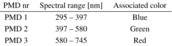
Table 1. Spectral range of the Polarisation Measurement Detector (PMD) channels.
PMD nr Spectral range [nm] Associated color
PMD 1 295 – 397 Blue
PMD 2 397 – 580 Green
PMD 3 580 – 745 Red
to the scattering properties of the cloud and the cloud cover, the situation with a completely covered sky and a low optical thickness can give the same radiance at the Top Of the Atmo-sphere (TOA) as the situation where there is a partial cloud cover and a higher optical thickness. While the radiance scat-tered in upward direction at the TOA is almost the same, the sensitivity of the GOME instrument changes significantly.
Satellites are better fit to produce regular cloud data with a global coverage for analysis of its distribution and trends than combining all surface observations alone. Since the beginning of the use of meteorological and research satel-lites, a number of methods have been developed to retrieve the cloud fraction and other parameters of clouds. In this study we are using data from ESA’s Global Ozone Mon-itoring Experiment (GOME). For cloud cover information from GOME data, there has been one retrieval method in use for some time by the GOME Data Processor (GDP): the Initial Cloud Fitting Algorithm (ICFA) based on work by Kuze and Chance (1994). In recent years at least three other methods were developed: the PMD (Polarisation Mea-surement Device) Cloud Recognition Algorithm (PCRA) by Kurosu and Burrows (1997), Kurosu and Burrows (1998), Kurosu et al. (1999) and von Bargen et al. (2000), the Opti-cal Cloud Recognition Algorithm (OCRA) by Loyola (1998) and von Bargen et al. (2000) and the Fast Retrieval Scheme for Clouds from the Oxygen A-band (FRESCO) by Koele-meijer et al. (2001).
In this study we evaluate the algorithms of the four cloud retrieval methods mentioned above, in order to better under-stand the consequences of their assumptions in their calcu-lated cloud fractions. We will present results of an intercom-parison of the cloud fractions retrieved by each of the four
methods with regular GOME pixels, but also compare the re-trieved cloud fractions from smaller PMD subpixels to obser-vations from synoptical surface weather stations. The PCRA and OCRAIMAU results used in this study are mainly from our own implementation based on the description of the al-gorithms in articles and reports because at the time when the study was performed no official version was available. In this final version of the paper we will also present OCRADLR re-sults from the version that is provided by von Bargen et al. (2000) for completeness. ICFA data is used from the GDP Level-2 product and FRESCO data was obtained from the Dutch SCIAMACHY Data Center. The time period used in our study are the months of August of 1997, 1998 and 1999. In Sect. 2 of this paper, the GOME instrument and the data that are used will be described, in Sect. 3 the various cloud fraction retrieval methods will be reviewed, and in Sect. 4 the results of the comparisons will be shown. Finally, Sect. 5 is for the conclusion of this work.
2 The GOME instrument
Fig. 2.Image showing the reflectance in 16 PMD sub-pixels inside each of a number of GOME pixels over the Netherlands (1 August 1997, pixel nrs: 480–510 (north to south), tracknr 104).
time of 10:30 AM. The orbits of three sequential days cover the whole Earth, making it possible to get global coverage from the GOME instrument (ESA, 1995).
3 Cloud fraction detection methods
3.1 Reflectance at the top of atmosphere
The upward radiation at the top of the atmosphere consists of backscattered light due to Rayleigh scattering from air molecules, Mie scattering from clouds and aerosols, and re-flected light from the surface of the Earth in the field of view. The radiation is measured by the spectral detector-array of the GOME instrument and by the broadband PMDs. These measurements are converted to albedo values by dividing the measured earth-shine by the solar irradiance and correcting for the length of the optical light path through the atmosphere due to solar zenith angleθ0(Eq. 2) and, in some cases, also adjusted with the line of sight angleθto the satellite (Eq. 2) which puts an emphasis on values retrieved from large view-ing angles:
ρ(λ)= π I (λ) F0(λ) cos(θ0)
(1)
̺(λ)= π I (λ) F0(λ) cos(θ0) cos(θ )
(2)
whereρ(λ)is the albedo and̺(λ)is the adjusted albedo at wavelengthλ(nm) for the detector array orλ=R, G, Bfor the broadband PMD channels,I (λ)is the upward radiance andF0(λ)the solar irradiance at the top of the atmosphere. 3.2 Initial Cloud Fitting Algorithm
The Initial Cloud Fitting Algorithm (ICFA), based on work by Kuze and Chance (1994) is used for the operational GDP Level-2 GOME data processor (DLR, 1994) and provides the standard GOME cloud fraction product for most users.
The ICFA method is based on a chi-square minimisation of high resolution measurements between 758–778 nm, com-prising of reflectances in the continuum and the O2A absorp-tion band (around 760 nm), and radiative transfer calcula-tions of a simulated cloud. The reflectivity of the wavelength region outside the O2A-band is mainly influenced by the cloud coverfc, the optical thicknessτand the surface albedo αs. The reflectivity inside the band depends on the cloud top height, the cloud fraction, the optical thickness and the surface albedo. This can be seen from Fig. 3, which shows the reflectance measured by the GOME instrument near the O2A-band: the clouded situation has a less deep O2A-band compared to the clear sky cases in the right panel of this fig-ure, because the cloud is blocking the absorption of light by the oxygen molecules below the cloud. The difference be-tween a land or sea surface does not matter significantly to the relative depth of the O2A-band. Due to the large size of the pixel, sets of GOME measurements are dominated by partially clouded scenes.
The simulated cloud reflectancesRsim(λ) is then written as:
Rsim(λ)=fc·Rcloud(λ) + (1−fc)·Rground(λ)
+Rclosure(λ) (3) wherefcis the cloud fraction and the other components are: Rcloud(λ)=α(µ, µ0)
Z
2(λ′−λ0)Tλ(Pc, µ, µ0)dλ′ (4) Rground(λ)=β
Z
2(λ′−λ0)Tλ(Pg, µ, µ0)dλ′ (5)
Rclosure(λ)=γ (1−λ/λ0) (6)
with µ0 and µ the cosine of the solar zenith angle and the viewing zenith angle, λ is the integration wavelength (758–778 nm), λ0 indicates some reference wavelength, 2(λ′−λ0)the entrance slit function,Tλ(Pc, µ, µ0)the trans-mission function of the atmosphere between the reflecting surface and the satellite,PgandPcthe ground and cloud top pressure, and finally there are three parameters used for the χ2minimisation in Eq. (7): α(µ, µ0)(the cloud top reflec-tivity),β (the ground reflectivity) andγ (a free parameter).
χ2= N X
i=1 "
Rmeas(λi)−Rsim(λi) ǫ(λi)
2
(7)
The factor ǫ(λi) denotes the errors in the individual re-flection measurements. Theχ2minimisation uses a set of pre-computed transmittances from a line by line code us-ing O2A-band absorption data from HITRAN ’96 (Rothman et al., 1998).
Because of the fixed optical thickness, the ICFA method produces an effective cloud fraction, i.e. a cloud fraction that corresponds to the radiances of a cloud with an optical thick-ness ofτ =20 and a cloud fractionfc.
The drawback of ICFA is that it uses the ISCCP monthly mean cloud top height database, which is a climatology based on measurements of clouds from satellites (MeteoSat, GMS, GOES and NOAA) between July 1983 and June 1991 (Rossow and Garder, 1993). This is seen as a strong short-coming of the algorithm. Although the monthly mean of cloud parameters in a grid-box may be reasonable accurate, it is likely that there is a difference between the actual cloud top height at a location at the moment of retrieval compared to the climatology. A comparison between ATSR-2 and ICFA effective cloud fractions has shown a mean difference of 18% with a standard deviation of 23% (Koelemeijer and Stammes, 1999b).
3.3 PMD Cloud Recognition Algorithm
The PMD Cloud Recognition Algorithm (PCRA) was first developed by Kurosu and Burrows (1997), later extended with the Revised Cloud Fitting Algorithm (RCFA) by Kurosu et al. (1999), and after that modified (von Bargen et al.,
2000). PCRA is capable of calculating the cloud fraction from GOME data and in combination with RCFA also the cloud top height and the optical thickness. We will only look at the cloud fraction part in this study.
Except for snow and ice surfaces, clouds generally have a higher reflectance than the Earth’s surface in the visual spec-tral range. By looking at the radiances detected by the PMDs, this can be used to distinguish between cloud and the surface if the reflectance of the surface is known.
A lookup table for each 0.5◦×0.5◦grid box (covering the Earth surface) was generated by processing all PMD pixels over a period of time (typically one month) and storing the minimum and maximum albedo of each of the three wave-length bandsλj =R, G, B(see Table 1) and a combination Zwhich is the ratio of the radiances ofλ=R andλ= G. All PMD sub-pixelsilocated in the same grid-box at(x, y) are evaluated to find the local minimum and maximum: ̺min(x, y, λj)=min ̺i(x, y, λj)
(8) ̺max(x, y, λj)=max ̺i(x, y, λj) (9) fori=1. . . n
̺min(x, y, Z)=min
̺i(x, y, R) ̺i(x, y, G) !
(10)
̺max(x, y, Z)=max
̺i(x, y, R) ̺i(x, y, G) !
(11) where the reflection̺(λ)is defined as in Eq. (2), andnis the total number of PMD sub-pixels in grid-box(x, y).
The minimum and the maximum albedo̺min,max(x, y, λj) of the PMDs, also called “thresholds”, represent a cloud free and a completely clouded situation respectively. Mar-ginsδcan be applied to the threshold values to account for different optical densities of clouds (maximum threshold), aerosol density, slightly changing surface reflectivity (min-imum threshold) and small changes in the solar zenith angle during the period the minimum thresholds were collected.
When the albedo of a PMD sub-pixel is above a maxi-mum value ̺max(x, y, λj)−δ or below a minimum value ̺min(x, y, λj)+δthe algorithm assigns these pixels a cloud fraction offc=1 orfc=0 respectively. All pixels that have not been classified by this method are interpolated linearly to a fractional cloud cover between minimum and maximum value (plus or minus the margin value):
fv(λj)=̺i(x, y, λ)− 1+δmin(λj)̺min(x, y, λj) (12) and also in case of sea:
fv(Z)=̺i(x, y, Z)− 1+δmin(Z)
̺min(x, y, Z) (13) or also in case of land:
fv(Z)= 1−δmax(Z)̺max(x, y, Z)−̺i(x, y, Z) (14) frange(λj)= 1−δmax(λj)̺max(x, y, λj)
− 1+δmin(λj)
fsubpixel(λj)=fv(λj)/frange(λj) (16)
fsubpixel= 1 4
X
λj=R,G,B,Z
fsubpixel(λj) (17)
fGOMEpixel= 1 16
X
k=1···16
fsubpixel,k. (18)
The wayfv(Z)is calculated for land and sea differs be-cause in cloud free situations over land more green than red light is reflected, and over seas this situation is reversed. The original PCRA uses a flow diagram (details in Kurosu and Burrows, 1997) for land and sea surface types determining the order of the wavelength bands on which tests are applied when calculating the cloud fractionfc. The most recent re-vision of the PCRA method (hereafter called PC2K) requires all channels and the ratio(R, G, B, Z)to be above or below the thresholds for a sub-pixel to be classified as cloudy or cloud free and sub-pixels that have PMD values inside the thresholds corrected by the margins are interpolated linearly like Eq. (12) and following equations for all channels.
The threshold databases are supposed to have attained their minimum and maximum values within a limited period of data because the vegetation and land use is seasonal de-pendent. This restricts the period of data that can be used for a minimum reflectance database to a month or a season at the most.
Therefore, the assumption that the minimum values have been reached may not be valid for all locations on Earth, es-pecially in regularly convective areas such as the tropics near the Inter Tropical Convergence Zone where clouds develop during the day and in other regions with a persistent cloud cover like the North Atlantic and North Pacific storm tracks, or polar regions with a persistent cloud cover that can last for long periods. This also affects OCRA (see next section), which uses the same historical cloud occurrence to make a similar cloud-free database.
PCRA has physically defined minima (clear sky thresh-olds) when the databases are created from sufficient data. One month is a good start for a 0.5◦×0.5◦ grid minimum threshold database, three months is more than sufficient for the mid-latitudes but shows some unusual areas of low re-flectance (“black spots”) in the minimum database that may eventually lead to incorrect results (although the minimum reflectance is less important than a well established maxi-mum). A problem for the interpretation of PCRA retrievals is that maxima of PCRA in the database correspond to a to-tally covered sky of an unknown cloud type and unknown cloud top height. As some types of cloud are more frequent in certain locations on Earth than others, this leads to a non-uniform cloud product when a short period of time is used to build the threshold database. The requirement to use long time periods to build a maximum threshold database con-tradicts with the requirement to shorten the period for the
building of the minimum threshold database due to the sea-sonality of land use. The effect of using data from a long period is also that the maximum thresholds are likely to be-come higher and the minima lower. The thresholds take more extreme values which leads to a shift towards the retrieval of optically thick clouds because they have a higher reflectance than thin clouds.
3.4 Optical Cloud Recognition Algorithm
OCRA stands for Optical Cloud Recognition Algorithm and was developed by Loyola (1997) (also Loyola (1998)). The cloud cover fraction is calculated by comparing the individ-ual PMD sub-pixel to the previously stored cloud free (CF) composite reflectance database. To get this cloud-free sur-face reflectance database, OCRA normalises the albedo val-ues calculated by Eq. (2) by dividing the red and green com-ponent by the sum of all three comcom-ponents:
r= X̺(x, y, λR)
j=R,G,B
̺(x, y, λj), g=
̺(x, y, λG) X
j=R,G,B
̺(x, y, λj) (19)
These r and g components are in normalised “rg-space”. Fromrandga vector−→rgcan be defined as the line between
the origin(0,0)and(r, g)with length||rg|| =pr2+g2. After normalisation, the distance in rg-space between the white point−→w, representing a white clouded pixel, and the
individual PMD sub-pixel−rg→i is calculated. The PMD albe-dos (Ri,Gi,Bi) of the pixel with the maximum distance to −
→
w are then stored in a database on a 0.5◦×0.5◦grid. The
maximal distance between−→w and the individual sub-pixel
− →
rgi at location(x, y)is given as in Eq. (20):
||−rg→CF(x, y)− −→w|| ≥ ||−→rgi(x, y)− −→w|| (20)
for i = ...n,
where−→rgCFis the cloud free situation and n the total number
of PMD sub-pixels in grid-box(x, y)that were used to make the cloud free composite.
The definition of “white” is an equal amount of radiation in all three wavelength bands (red, green and blue). From this definition it can be easily shown that “white” in rg-space is−→w =(rwhite, gwhite)=(13,13).
After the cloud free composite has been made, the calcu-lation of the cloud fractionfc of a GOME pixel is done by calculating the fractions of the individual PMD sub-pixelsi and then averaging over all 16 sub-pixels in a GOME pixel: fi(λ)=max0, S(λ)(̺i(x, y, λ)−̺CF(x, y, λ))2−O(λ) (21) forλ= R, G, B
Fc,i= s
X
λ=R,G,B
fi(λ) (22)
fc= 1 16
X
i=1···16
Fig. 3. Left: Reflectance measured by GOME near the O2-A absorption band. The dotted line is a fully clouded scene, the solid line is
a clear sky situation over land (the Netherlands), the dashed line is a clear sky situation over sea (the Atlantic Ocean). Right: Normalised albedo of the same situations (normalisation wavelengthλn=758.0 nm).
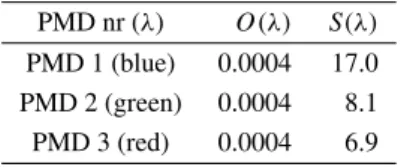
Table 2. The OCRAIMAUoffset factorsO(λ)and scaling factors
S(λ)per PMD channel used in this study.
PMD nr (λ) O(λ) S(λ)
PMD 1 (blue) 0.0004 17.0
PMD 2 (green) 0.0004 8.1
PMD 3 (red) 0.0004 6.9
whereS(λ) is a scaling factor andO(λ)is an offset. Both S(λ) and O(λ) are empirical factors, which can be deter-mined using only GOME PMD data (as the official algorithm does) or based on a comparison with other data. For the runs with our in-house developed implementation of OCRA (in-dicated with OCRAIMAUin next sections), data from ICFA was used to find a set of offset and scaling factors (Ta-ble 2): the offsets were found minimising the difference be-tween the calculated PMD cloud fraction and clear sky pixels (fc=0.0) and the scaling factors were found minimising the difference between the median of the PMD based cloud cover frequency diagram aroundfc=1.0 for clouded pixels.
It should be noted that the offset and scaling factors in von Bargen et al. (2000) (which we will call the “DLR-implementation” or “OCRADLR” in the following sections of
the paper) are considerably different from the values in Ta-ble 2. Most likely this is caused by the different dataset or methods used for the optimisation of these factors.
The scaling factors effectively define the cloud that is rep-resented by OCRA: a lowerS(λ)lowers the cloud fractions, thus representing all clouds as with a higher effective opti-cal thickness and a higherS(λ)does the opposite. The offset factorsO(λ)function as an additional threshold to account for aerosols and other effects unrelated to clouds that can in-crease the radiation.
The OCRA method has been implemented in the devel-opment version of the GOME Level 1-to-2 Data Processor
and may be used as the default cloud fraction product in the future (von Bargen et al., 2000).
The authors of this paper think that there are a couple of issues with the OCRA retrieval method. The method that OCRA uses to arrive at a cloud free reflection database is based on getting the point furthest away from “white” in nor-malised rg-space, aiming to reach a value that will be cloud free and which also has the lowest reflection. The normalisa-tion method uses the ratio of the reflecnormalisa-tions measured by the PMD channels and has lost information about the absolute value of the reflection itself. This normalisation and search mechanism does therefore not guarantee that the saved PMD values are indeed cloud free and correspond to the lowest reflectance available, although this minimum reflectance is required in the cloud fraction calculation phase.
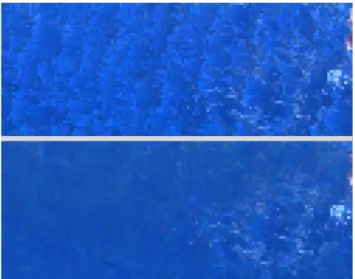
Visual inspection of the cloud free database of OCRA (made with this “furthest from white” method) shows a “patchy” surface, while the PCRA minimum thresholds, which is a combination of independently ranked PMD chan-nels, provides a more smooth image of the Earth. An exam-ple of this is shown in Fig. 4, where the three PMD com-ponents of the cloud-free database of OCRA and minimum thresholds of PCRA of a part of the Pacific Ocean are de-picted in RGB color with equal scaling with respect to signal strength. These minimum threshold images were made using one month of data in August, but also three-year compos-ites of August months show the same patchy behaviour from grid point to grid point in OCRA and did not seem to im-prove to the level of smoothness of a one-month PCRA min-imum threshold image. Although the Cloud Free database that comes with OCRADLR uses a complete year of PMD
The OCRA algorithm heavily depends on the scaling and offset factors to calculate the cloud fraction. The selection mechanism of the pixels that are used and the exact criteria for the histogram analysis determine what PMD intensity the algorithm will classify as a fully covered or cloud free PMD pixel. This means that for different sets of input data different factors may be produced, which makes the algorithm less uniform.
3.5 Fast Retrieval Scheme for Clouds from the Oxygen A-band
The Fast Retrieval Scheme for Clouds from the Oxygen A-band (FRESCO) developed by Koelemeijer et al. (2001) is capable of calculating cloud fractions and the cloud top height. It uses the radiances in wavelength regions of 1 nm wide inside and outside the O2A-band: at 758 nm where there is no absorption, at 761 nm where there is strong ab-sorption and at 765 nm where the abab-sorption is moderate. A number of assumptions are made: absorption by gases occurs only by O2 above clouds or the ground surface, scattering processes by air molecules and aerosols are neglected inside and below the cloud, and both the surface and the cloud top are assumed to be Lambertian reflectors. A simulation of the reflectanceRsim at the top of the atmosphere consists of a clear part with surface albedoAs and a clouded part with the cloud albedoAc(the weighted plane-parallel approach): Rsim=(1−fc) T (λ, ps, θ, θ0) As+fcT (λ, pc, θ, θ0) Ac(24)
where fc is the cloud fraction, T the transmittance, λ the wavelength,ps andpc are the surface and cloud top pres-sure,θandθ0are the line of sight and solar zenith angles re-spectively. The absorption is calculated using HITRAN ’96 data and a mid-latitude summer atmosphere Anderson et al. (1986). The surface albedo is taken from a minimum re-flectance database on a 2.5◦×2.5◦ grid from GOME mea-surements using all data in the months of January and July, the sea surface albedo is taken as 0.02, and the cloud albedo is taken as 0.8. A non-linear least-squares minimisation is used to derive the cloud fraction and the cloud top pressure. For this minimisation the Levenberg-Marquardt method is used Press et al. (1986).
The assumption of a fixed cloud albedo means that FRESCO works with an effective cloud fraction for clouds with an albedo of 0.8. This corresponds with a cloud with an optical thickness τ of about 50 for a solar zenith angle θ0 = 0◦or smaller values forτ for increasing solar zenith angles (Los et al., 1997).
The most important difference between FRESCO and ICFA (which also uses wavelengths around the O2A-band) is that FRESCO determines the effective cloud fraction and the cloud top pressure at the same time, where ICFA deter-mines only the effective cloud fraction.
The authors think that the largest drawback of FRESCO is its clear sky surface albedo database, which has a large grid
Fig. 4. An RGB image of the minimum reflectance surface databases of an area between 0S - 25S and 145W - 80W (Pacific Ocean) for OCRA (top) and PCRA (bottom).
cell size of 2.5◦×2.5◦. The surface characteristics may dif-fer considerably within such a large area which may increase the uncertainty in areas of mixed surface type (e.g. coasts, mixed agricultural and urban areas). Also, the spectrometer of GOME is known to degrade and the spectral characteris-tics of the clear sky database may change over time. This can also be a point of concern for the ICFA method, but not for PCRA and OCRA which use a threshold database that is restricted in time.
3.6 Synoptic surface observations
Synoptic surface observations are made by human eye at most operational weather stations. They provide a cloud frac-tion in octas (steps of 18) and the type of the most dominant cloud. Zero octas corresponds to a clear sky and eight oc-tas corresponds to a completely covered sky. These synoptic observations are estimated to be representative for an area with a radius of 20–30 km (Rossow et al., 1993, and refer-ences therein) which corresponds roughly with the size of one PMD sub-pixel of 20×40 km2.
In the comparison of surface observations with satellite based retrieval methods the location of the surface station has to be co-located with the (sub-)pixel. Also, as an ad-ditional requirement, the satellite over-pass must be within 30 minutes on either side of the moment of observation at the surface station. This is to minimise possible differences in cloud type due to advection: if the wind is blowing with a speed of 10 ms−1parallel to the scan direction of the GOME instrument scan mirror (often east-west direction), all the clouds in one PMD pixel have moved to the adjacent PMD pixel in only 30 minutes.
Table 3.Cloud classificationCfrom the 8NsChshs SYNOP code
group.
Nr Type Nr Type
0 Cirrus (Ci) 5 Nimbostratus (Ns)
1 Cirrocumulus (Cc) 6 Stratocumulus (Sc)
2 Cirrostratus (Cs) 7 Stratus (St)
3 Altostratus (As) 8 Cumulus (Cu)
4 Altocumulus (Ac) 9 Cumulonimbus (Cb)
the time difference is large or if the station is located at the border of the PMD pixel.
The cloud classification comes from the so called 8NsChshs indicator (or sometimes 8NhCLCMCH) in SYNOP weather reports, where “8” is the group-indicator, Ns indicates the cloud cover fraction of the most dominant cloud typeCs described in Table 3.
One of the problems of comparing SYNOP surface mea-surements to satellite derived meamea-surements is that, while looking at the same cloud, the determined cloud fraction may be different. Part of this difference may be explained by tak-ing into account the distance of the cloud layer to the ob-server and the path through which it is observed: for the hu-man observer on the ground the cloud is at a few hundred meter or a few kilometer in altitude, seen through the hazy boundary layer which limits the observer to about 20–30 km radius, while the satellite instrument observes the same cloud from above at 800 km altitude, through mostly optically thin air. An other issue is the definition of a cloud: a hu-man observer may define a cloud as the portion of the sky that is “white” on a blue-ish background, while the satellite instrument is using calibrated spectral radiances or broad-band measurements. Cloud fractions reported in the SYNOP reports are classified by the eye of humans and, although trained for this work and following standards set by the WMO, the results may differ per individual. A satellite in-strument stays the same, and should give similar results in similar cases in all parts of the world (when degradation of the instrument is not taken into account). Cloud fractions re-ported by surface observers are supposed to be independent of the cloud optical thickness but geometrical effects with clouds with a larger vertical structure may increase the re-ported cloud cover.
3.7 Snow and ice
The retrieval of the cloud fraction in all four retrieval meth-ods above are limited over highy reflecting surfaces, such as snow and ice, or situations where there is sunglint over water. The light that is reflected to the satellite by these high reflecting surfaces is so intense that a meaningful sig-nal from a cloud above the surface can’t be distinguished
from the surface reflection itself with the current methodol-ogy. A permanent coverage of the surface by snow and ice will cause high PMD values to be stored in the minimum-reflectance database of PCRA and OCRA and subsequently interfere with the retrieval of the cloud fraction. A surface type mask of these high reflecting surfaces is therefore used to flag the results.
With other methods, such as the use of O4absorptions,it may be possible to retrieve clouds above snow and ice sur-faces. This approach is being explored for GOME and SCIA-MACHY retrievals and may improve trace gas retrievals above polar areas (Wagner et al., 2002).
3.8 Cloud top height
Although the focus of this paper is a discussion of cloud cover fraction algorithms, we can’t avoid touching briefly on the retrieval of cloud top height and optical thickness, be-cause these three parameters together determine for a large part the reflection from clouds measured by the satellite at the top of the atmosphere.
In its retrieval of the cloud fraction, the ICFA method uses the cloud top height information from ISCCP (whose val-ues are also provided in the GDP Level-2 product). The FRESCO algorithm retrieves the cloud top height at the same time as the cloud fraction via a non-linear least squares method (described in Sect. 3.5), which keeps these two re-trieved parameters consistent. The retrieval of cloud top height and optical thickness for PCRA and OCRA is done via the RCFA algorithm. RCFA is a second-stage algorithm, designed to run after the cloud cover fraction retrieval and uses the retrievedfc as an input parameter. The cloud top height in RCFA is basically calculated from the depth of the oxygen-A band, which has a low sensitivity to errors in the cloud fraction (von Bargen et al., 2000). However, for the cloud optical thickness, the effect of an error in the cloud fraction is significant due to the dependency of the albedo at the top of the atmosphere on the cloud fraction. Differences inτ of 5–9 are possible (von Bargen et al., 2000), which means that for many common types of clouds the retrieval error is as large as the optical thickness of the true cloud (see Table 4)
Fig. 5.Position of the centre of the GOME pixels above the Nether-lands used in this section for the months of August 1997 (87 pixels), August 1998 (92 pixels) and August 1999 (102 pixels).
3.9 Data sources
The data we used for this paper is from the months of Au-gust 1997, 1998 and 1999 in which a number of GOME pix-els located near the Netherlands were selected (Fig. 5). The clear sky composites for PCRA and OCRAIMAUwere made for each of the three years using all PMD data in August of that particular year. The OCRADLR cloud free database was the default that came with the ESA report (von Bargen et al., 2000) The ICFA values are taken from the most recent revision of the GDP Level-2 data (R02) and the FRESCO data comes from the Dutch SCIAMACHY Data Center. The synoptic surface observations used in the comparisons are from weather stations within the Netherlands and some ob-servations from ships on the North-Sea that were collected at 10:00, 11:00, and 12:00 hrs UTC.
4 Results
4.1 Comparison for different types of clouds
In Sects. 3.2 and 3.5 we have seen that ICFA and FRESCO use a fixed optical thicknessesτ of 20 and about 50 respec-tively in their calculations of the cloud fraction, independent of the type of cloud. For PCRA/PC2K and OCRA the cloud fraction is determined by the threshold database and the off-set and scaling factors, also independent of the type of cloud.
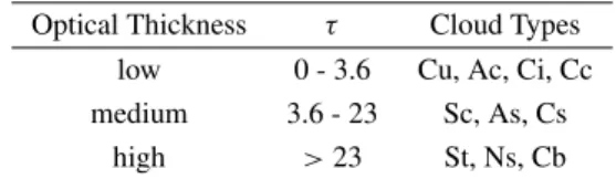
Table 4. Clouds divided by class of optical thickness (after von Bargen et al., 2000).
Optical Thickness τ Cloud Types
low 0 - 3.6 Cu, Ac, Ci, Cc
medium 3.6 - 23 Sc, As, Cs
high >23 St, Ns, Cb
A human observer however, can both estimate the cloud frac-tion and classify types of clouds with different optical thick-nesses.
To study the effect that different types of clouds can have on the retrieved cloud fraction, we separate the clouds by class of optical thickness following Table 4. Figure 6 shows the comparison of PC2K cloud fractions with surface ob-servations for co-located sub-pixels which are separated by cloud type (top), and the frequency analysis of the cloud frac-tions respectively (bottom).
The frequency distribution in the left histogram panel shows that clouds with a low optical thickness and a large fractional cover are represented by the retrieval algorithm as a thick cloud with a small cloud fraction. The centre plot shows that clouds with a medium optical thickness are also represented by a cloud with a smaller fractional cover than observed from the surface, although the mis-match is less strong. The number of data points with thick clouds is, re-grettably, very small.
The reducing mis-match of the frequency diagrams of the retrieved clouds with a low to medium optical thicknesses is in accordance with the expected smaller amount of radia-tion from these clouds with the same cloud cover compared to optically thick clouds, which reflect much more light to the satellite instrument. Since PC2K interpolates the cloud fractions between the minimum and the maximum value in the threshold database, cloud fractions of clouds with a low optical thickness are scaled to a thick effective cloud.
Fig. 6.Top: Individual PC2K cloud fractions against the co-located surface observations, separated by cloud class. Left: thin clouds; centre: medium optical thickness clouds; right: thick clouds. Bottom: Frequency histogram of the cloud fractions. Solid line: individual PC2K cloud fractions; dashed line: cloud fractions of co-located SYNOP observations. All data in August 1997, 1998 and 1999 are used.
PC2K the effective cloud fraction scaling only takes effect if the maximum threshold was created with sufficient data to ensure a complete cloud cover to be stored in the database. 4.2 Comparison of the retrieval methods and SYNOP with
ICFA
The ICFA cloud fraction is at this moment the standard retrieved cloud fraction from the operational GOME GDP Level-2 data product and, therefore, first the comparison be-tween ICFA and the other retrieval methods will be presented as a baseline (see Fig. 7), as well as the comparison between ICFA and SYNOP surface measurements (Fig. 8).
In Fig. 7, the cloud fractions retrieved with PCRA/PC2K and OCRA in a GOME pixel are averaged over all 16 PMD sub-pixels, whereas FRESCO is one value for the complete GOME ground pixel. The error bars on the ICFA values are the uncertainties according to the GDP Level-2 data product. A margin of 5% was applied to the absolute values of the top and bottom PCRA thresholds for PMD channelsλ = R, G andB, and a margin of 0% was taken for the ratioZ. The margin forZis set to zero because the effect on the selection of cloud fractions offc =0 andfc =1 is very much influ-enced by the value ofZitself, due to its higher absolute value (on average 0.6 ≤ Z ≤ 1.1) and corresponding larger mar-gins of the minimum and maximum thresholds compared to the margins of regular PMD channels. Generally, values for measured PMD range between 0.02≤λ=R, G, B≤0.27. Therefore, the measured value of a PMD subpixel would more likely be in the margin zone ofZthan the other chan-nels and this would cause an unnatural shift tofc = 0 or fc =1, if the margin forZwas taken 5% as well. For the comparison between PC2K and ICFA, a margin of 5% was applied to all thresholds for PMD channelsλ = R, Gand Band for the ratioZas well (in contrast to the earlier PCRA method).
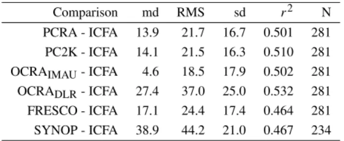
Table 5. The mean difference (md) in %, the root-mean-square (RMS) in %, the standard deviation (sd) in %, the correlation coef-ficient (r2) and the number of cases (N) of the comparison between ICFA and other retrieval methods and SYNOP surface observations, taken over all three years.
Comparison md RMS sd r2 N
PCRA - ICFA 13.9 21.7 16.7 0.501 281
PC2K - ICFA 14.1 21.5 16.3 0.510 281
OCRAIMAU- ICFA 4.6 18.5 17.9 0.502 281
OCRADLR- ICFA 27.4 37.0 25.0 0.532 281
FRESCO - ICFA 17.1 24.4 17.4 0.464 281
SYNOP - ICFA 38.9 44.2 21.0 0.467 234
Table 5 contains the statistics of the comparisons in Figs. 7 and 8. Positive values of the mean difference indicate that the method mentioned first in the table has larger cloud fractions. The table shows that the ICFA cloud fraction method gener-ally gives lower values than the other retrieval methods and the surface observations. It has already been indicated that ICFA also gives lower cloud fractions than the monthly mean ISCCP values (Koelemeijer and Stammes, 1999b). The over-estimation of ISCCP was attributed to the threshold methods used to select between clear sky and (partly or fully) clouded pixels. Since partially clouded pixels would be classified as completely clouded, ISCCP is biased towards higher cloud fractions.
Fig. 7.A comparison of the cloud fraction averaged over all PMD sub-pixels in a GOME pixel against ICFA for the months of August 1997,
1998 and 1999. Top-left: PCRA, top-right: PC2K, centre-left: OCRAIMAU, centre-right: OCRADLR, bottom: FRESCO. The dashed line is
the linear regression through the points in the domain, the solid line indicates unity.
PC2K has changed the algorithm, but apparently has no sig-nificant impact on the results. We draw the conclusion that both methods are interchangeable. For the following com-parisons we will skip PCRA method and only present PC2K results, which is the most recent version of the algorithm.
The IMAU-implementation of the OCRA algorithm has the lowest mean difference and RMS and a standard devia-tion comparable to PC2K and FRESCO. The small mean dif-ference and RMS are because the offset and scaling factors in Table 2 were determined using ICFA measurements, so this is not unexpected. However, the DLR-implementation of the OCRA algorithm produces a mean difference that is more than 10% larger than the other three retrieval methods. The RMS and the standard deviation of the comparison are
con-siderably larger as well. We note that the difference between the results from the OCRAIMAUand OCRADLR implemen-tations is very large, and we think the different offset and scaling factors are the main cause for this.
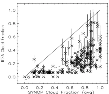
Fig. 8. A comparison between the cloud fraction from averaged co-located surface observations (SYNOP) against ICFA for August 1997, 1998 and 1999.
The generally smaller cloud fraction of ICFA compared to the three other retrieval methods may be due to different causes. PC2K uses a maximum threshold database which represents a complete cloud cover at each 0.5◦×0.5◦ grid-box, but there is no precise information on the optical thick-ness or the type of cloud that provided this maximum reflec-tivity. When the effective optical thickness of the maximum cloud cover is less thanτICFA=20, cloud fractions from the PCRA method will be larger than ICFA for the same situa-tions. The considerably larger values from OCRADLR indi-cate that its scaling factors also result in an effective cloud fraction that is less thanτICFA. A set of lower scaling fac-tors would reduce the mean difference but not necessarily the RMS. Finally, the reason for the general larger cloud frac-tions from FRESCO is that it fits cloud fraction and cloud top height at the same time while using a cloud with an ef-fective optical thickness aroundτFRESCO = 30 ∼ 50. A comparison of the cloud top heights provided in the GDP Level-2 data product with those retrieved by FRESCO shows that the FRESCO cloud top height is generally lower than the value ICFA uses from the ISCCP database. A lower cloud top height gives a lower reflectivity at TOA and the cloud frac-tion needs to increase to compensate to get the same radiafrac-tion at the satellite.
The comparison of averaged co-located SYNOP ground observations with ICFA indicates that the cloud fraction re-ported by the surface observer is in most cases much larger than the cloud fraction of ICFA: the mean difference is 39%. The reason for this large difference may be dominated by their different spatial extensions. The number of surface ob-servations in a GOME pixel is generally small (2 to 6) com-pared to the 16 PMD sub-pixels within a GOME pixel. If
one takes into account the area for which the surface obser-vation is representative (radius 20–30 km) and compares this to the size of the GOME pixel (320×40 km2), the overlap between the GOME pixel and the represented areas by the surface stations is often not sufficient. The estimate the ob-server makes of the cloud cover may have been influenced by the geometry of the cover, especially in cases of broken clouds where visible vertical sides of a cloud contribute to the covered area in the field of view. This contribution will be in the direction of an overestimation of the observed cloud frac-tion. Although the GOME instrument also looks at ground pixels from an angle (max±30◦), this angle is smaller than the 90◦from zenith to the horizon that surface observer has to take into account.
4.3 Comparison of the methods against SYNOP surface observations using pixels near the Netherlands In this section we compare the results of the retrieval meth-ods with SYNOP data because the latter is a non-satellite based value that best matches the area of a PMD pixel in the PC2K and OCRA retrieval methods. In the left panels of Fig. 9, the comparison is shown between cloud fractions of individual PMD sub-pixels from PC2K and from FRESCO and in Fig. 10 the two OCRA versions versus the co-located individual SYNOP surface observations (indicated with “ind. co-locations” in Table 6). In the right panels, all available sets of PMD/SYNOP co-locations in a GOME pixel are av-eraged (cases “avg. co-locations”). The last type of cases in Table 6 is “avg. over GOME pixel”, wherein the average of all 16 PMD sub-pixels is compared with all available co-located SYNOP observations. In this comparison also the PMD subpixels without a co-located synoptical observation are taken into account. The values of the individual SYNOP observations on the vertical axis are fixed to “strata” of mul-tiples of octas (= 18 of the hemisphere), where zero octa (08) is a clear sky and eight octa (88) means completely covered. The averaging (on the right) wipes the stratification as all co-located observations within a GOME pixel are taken into account.
Fig. 9. A comparison between the cloud fractions of the individual PMD sub-pixels against individual co-located SYNOP surface obser-vations (top-left) and averaged over a GOME pixel (top-right) for August 1997, 1998 and 1999 for PC2K and the FRESCO cloud fraction against individual SYNOP observations (bottom-left) and averaged (bottom-right).
Fig. 10.A comparison between the cloud fractions of the individual PMD sub-pixels against individual co-located SYNOP surface
Table 6. The mean difference (md) in %, the root-mean-square (RMS) in %, the standard deviation (sd) in %, the correlation coef-ficient (r2) and the number of cases (N) of the comparison between SYNOP and retrieved cloud fraction methods, taken over all three years. Case description in the text.
Comparison md RMS sd r2 N
ICFA - SYNOP −38.9 44.2 21.0 0.467 234
PC2K - SYNOP
ind. co-locations −25.3 33.7 22.1 0.469 662
avg. co-locations −24.4 30.6 18.3 0.596 234
avg. GOME pixel −22.9 29.3 18.1 0.603 234
OCRAIMAU- SYNOP
ind. co-locations −33.7 41.5 24.1 0.462 662
avg. co-locations −32.7 38.3 19.9 0.576 234
avg. GOME pixel −31.9 36.8 18.3 0.607 234
OCRADLR- SYNOP
ind. co-locations −8.8 30.6 29.3 0.553 662
avg. co-locations −9.5 24.4 22.5 0.684 234
avg. GOME pixel −10.0 23.3 21.1 0.645 234
FRESCO - SYNOP
ind. co-locations −20.2 29.1 21.0 0.496 662
avg. GOME pixel −19.7 27.5 19.1 0.559 234
all PMD sub-pixels and all co-located surface observations in a GOME pixel does not change the mean difference signifi-cantly. While the comparison between individual co-located surface observations and the FRESCO value is given, the av-eraged observation comparison gives a better indication be-cause an individual sub-pixel is not representative for the whole GOME pixel.
The overestimation of surface observations compared to satellite measurements has also been noted in the ISCCP study, where a comparison between 3-hr global satellite cloud fraction data and over 670 000 surface observations was performed. An average overestimation of 11% and a standard deviation of 40% was found and this difference was reported to be seasonal dependent (Rossow et al., 1993).
A comparison of PC2K and OCRA (the DLR-implementation) with high spatial resolution ATSR-2 cloud fractions (von Bargen et al., 2000) gave RMS errors of 27.5 and 27.1 respectively, which is lower than our comparison against SYNOP observations.
4.4 Comparison of the methods against each-other In this section we directly intercompare the retrieved cloud fraction results from PC2K, OCRA and FRESCO. This is done both on a small (PMD-size) scale, and averaged over a GOME pixel, e.g. where compared to FRESCO. Statistics from the comparisons in this section are printed in Table 7
where individual PMD comparisons are indicated with “ind.” and those where 16 pmd pixels are averaged with “avg.”
Figure 11 shows the retrieved cloud fractions from the PC2K method against the two implementations of OCRA. The most significant difference between the two left pan-els is the steep slope of the OCRADLRimplementation from fc =0–1 where PC2K went fromfc =0 to 0.5, compared to the saturation of OCRADLRatfc =1 where PC2K has a range offc = 0.5–1. The comparison of OCRAIMAUwith PC2K is much closer to the unity line, although PC2K has slightly larger cloud fractions than OCRAIMAU (mean dif-ference is 9.5%). Averaging the 16 PMD subpixels in each GOME pixel leads to a less wide spread of points (i.e. the RMS and standard deviation in the averaged values drop) and a less steep slope of OCRADLR due to the inclusion of some of the “saturated” cloud fraction pixels in the average, which pulls the result more towards the unity line. Note that the unity line does not necessarily represent the “true” cloud fraction, in the plots presented in this paper it serves as a guide line to see how much agreement there is between re-trieval methods.
In Figure 12 the retrieved cloud fractions from both OCRA implementations are intercompared. Here also, the DLR-implementation shows a rapid change from cloud free to completely cloud covered, as wel as the saturation of the cloud fraction abovefc=0.4 compared to OCRAIMAU. The reason for this must be the different scaling set of factors, as theseSλ factors effectively determine at what PMD sig-nal value a cloud is represented as completely covered. This comparison, together with Fig. 11, indicates that the Sλ of OCRADLRare too large to produce a cloud cover comparable to our PC2K version or the OCRAIMAUimplementation. The two tested OCRA implementations retrieve a cloud fraction for the same PMD pixel that has a mean difference of 23% over 4496 PMD pixels (or 281 complete GOME pixels).
Figure 13 shows the cloud fractions of the three PMD retrieval methods/implementations in comparison with FRESCO. For this comparison all PMD pixels in each GOME pixel are averaged. The saturation of OCRADLRis again visible when compared to FRESCO. OCRAIMAU pro-duces smaller cloud fractions than FRESCO in most cases, with a mean difference (MD) of 12%. The comparison of PC2K cloud fractions and FRESCO is close, with a MD of only 3%, due to similarities in the methods.
4.5 Comparison of data over a track
In this section we will compare the cloud fractions from the retrieval methods along four tracks to study the consistency of the results for the same cases over a wider range of surface types and cloud situations.
Fig. 11. A comparison of the cloud fraction of the individual PMD sub-pixels of the PC2K method against the OCRADLR(left-top) and
averaged over the GOME pixel (top-right). Same for OCRAIMAU(bottom left and right). Time period and pixels are the same as in Sects. 4.3
and 4.2.
Fig. 12.A comparison of the cloud fraction of the individual PMD sub-pixels of the OCRAIMAUmethod against the OCRADLR(left) and
averaged over the GOME pixel (right). Time period and pixels are the same as in Sect. 4.3.
(northern and southern) Atlantic Ocean, the northern At-lantic Ocean and South America, and the last track runs over a part of New-Foundland, the northern Atlantic Ocean, the Caribean Sea, a small part of South America and finally over the southern Pacific Ocean. Figure 14 contains the cloud fractions of the nadir pixels from ICFA, PC2K, FRESCO and of the two OCRAIMAU, OCRADLR implementations along track “70802101” as an example.
The mean cloud fraction and the standard deviation are given in Table 8 as a total over all 4 tracks. The cloud frac-tions produced by ICFA are generally the lowest (24%
Fig. 13.A comparison of the cloud fraction of the PMD methods (OCRAIMAU, OCRADLRand PC2K) against FRESCO averaged over the
GOME pixel. Time period and pixels are the same as in Sect. 4.3.
Fig. 14. Cloud fraction of the nadir pixels along GOME track “70802101” on 2 August 1997. Top panel: cloud fraction of ICFA (solid),
Table 7. The mean difference (md) in %, the root-mean-square (RMS) in %, the standard deviation (sd) in %, the correlation co-efficient (r2) and the number of cases (N) of the retrieved cloud fraction methods compared against each-other, for the same pixels as above, taken over all three years. Case description in the text.
Comparison md RMS sd r2 N
PC2K - OCRADLRind. −13.2 27.3 23.9 0.768 4496
PC2K - OCRADLRavg. −13.2 21.2 16.5 0.883 281
PC2K - OCRAIMAUind. 9.5 14.9 11.4 0.869 4496
PC2K - OCRAIMAUavg. 9.5 11.6 6.6 0.936 281
OCRAIMAU- OCRADLRind. −22.7 32.6 23.3 0.738 4496
OCRAIMAU- OCRADLRavg. −22.7 27.8 15.9 0.845 281
OCRAIMAUavg. - FRESCO −12.5 13.9 6.09 0.944 281
OCRADLRavg. - FRESCO 10.3 20.4 17.7 0.824 281
PC2K avg. - FRESCO −3.0 7.6 7.0 0.907 281
Table 8.Mean cloud cover fraction (mean) in %, the absolute dif-ference (diff) to ICFA in %, the standard deviation (sd) in % and the number of pixels (N) of the comparison along the four tracks.
Case mean diff sd N
ICFA 24.1 – 26.3 1845
PC2K 39.2 15.1 22.7 1845
OCRAIMAU 26.1 2.0 22.7 1845
OCRADLR 49.7 25.0 35.5 1845
FRESCO 34.2 9.5 24.7 1725
Shown in Fig. 14 between 20N–10N, the FRESCO method retrieves a cloud fractionfc∼0.3 where all the other meth-ods retrieve a clear sky. The soil surface along this part of the track is dry Sahara desert changing to Sahel further south. A possible explanation for the elevated cloud fraction may be the higher albedo of sand and aerosols over the desert that give a higher reflection than the 2.5◦×2.5◦surface database corrects for, thus leading to a residue signal which is in-terpreted as a cloud. Here the size of the albedo grid cell may hinder the retrieval if the surface type changes too much over the grid box (vegetation in the Sahel region has a lower albedo than the Sahara desert). The other retrieval methods benefit from a smaller albedo grid size wherein the changes with respect to location are smaller. At several other areas along the tracks the ICFA cloud fraction is much lower than the cloud fraction of PC2K, OCRADLR,IMAU or FRESCO. For instance around 50N and between 7S–25S along track “70802101”. A possible reason for this difference may be an incorrect cloud top height (taken from the climatology database) as most of these track-pieces are sea pixels which have a relatively low surface reflection.
In Table 9 the numerical mean difference, the RMS and
Table 9. Mean difference (md) in %, RMS in %, the standard de-viation (sd) in % and the number of pixels (N) of the comparison along the tracks.
Case mean RMS sd N
ICFA - PC2K −15.1 26.9 22.2 1845
ICFA - OCRAIMAU −2.0 22.1 21.0 1845
ICFA - OCRADLR −25.0 36.7 26.0 1845
ICFA - FRESCO −9.5 22.7 20.6 1725
FRESCO - PC2K −4.2 11.6 10.8 1725
FRESCO - OCRAIMAU 8.4 11.5 7.9 1725
FRESCO - OCRADLR −14.3 24.8 20.3 1725
PC2K - OCRAIMAU 13.1 16.6 10.1 1845
PC2K - OCRADLR −9.8 23.9 21.8 1845
the standard deviation of the difference of the various meth-ods are given. We note again that the optimisation of the offset and scaling factors of OCRA gives a low mean dif-ference but the RMS is comparable to the other ICFA cases. FRESCO and PC2K show a small mean difference, RMS and standard deviation, which may be caused by the similarity of the used methods: interpolation between clear sky minima from a grid and a fixed maximum or grid maximum, both with radiance characteristics of a thick cloud. The differ-ence between the two OCRA implementations is apparent in both the bottom panel of Fig. 14 and in the table containing the statistics. The OCRADLRretrieves a significantly larger cloud fraction, which is predominantly determined by the scaling factor S(λ)per PMD. A larger scaling factor leads to the effect that a reflected radiance from the earth of a cer-tain magnitude will sooner reach a cloud fraction fc = 1 than with smaller scaling factors. When OCRADLR is al-most always larger than ICFA, this leads us to the conclusion that, when cloud top height is not taken into account, the cloud fraction that OCRADLRrepresents is associated with a smaller cloud optical thickness thanτ =20, the standard used in ICFA.
5 Conclusions
We have described the ICFA, PCRA/PC2K, OCRA and FRESCO cloud fraction retrieval methods for GOME. For this purpose we intercompared the retrieved cloud fractions of these methods together with co-located synoptical surface observations over the Netherlands for August 1997, 1998 and 1999.
effective high optical thickness. This can also be the reason for the wide spread of solutions for retrieved cloud fractions compared to surface observations with a cloud fractionfc> 0.4.
In general, we found that, along four processed GOME tracks, ICFA produces the lowest cloud fractions, followed by the OCRAIMAU implementation, then FRESCO, PC2K and finally the OCRADLR implementation (+2%, +10%, +15% and +25%, compared to ICFA respectively). A com-parison between synoptical surface observations of clouds by human eye and retrieved cloud fractions from GOME PMD pixels of roughly the same size showed that the surface obser-vations typically have a larger cloud fraction than the satellite cloud fraction retrieval methods. With respect to SYNOP, the OCRADLR algorithm has a cloud fraction that is about 9% lower (mean difference), followed by PC2K and OCRAIMAU (25% and 34% lower respectively, compared to SYNOP).
Concerning the OCRA method, the authors think that the method to find the Cloud Free database by normalisation of the radiances produces an unnatural patchy behaviour. The method further depends heavily on a proper determination of the set of scaling and offset factors as shown by the differ-ences in the results of the DLR and our own implementation. The offset and scaling factors are not necessarily the same for different optimisation datasets, which makes the use of OCRA difficult. For PCRA/PC2K the maximum thresholds in each gridbox can differ and represent a cloud with un-known properties. This also makes the use of this method difficult. At present, the authors have the opinion that, the FRESCO cloud retrieval algorithm provides a consistent set of cloud parameters (fc,τ and cloud top) due to its simulta-neous retrieval.
Acknowledgements. The authors wish to thank ESA for providing
the GOME data, the Dutch SCIAMACHY Data Center for making the FRESCO data available, NWO/SRON for their financial support of this project and colleagues for their support preparing this paper.
References
Anderson, G., Clough, S., Kneizys, F., Chetwynd, J., and Shettle, E.: AFGL atmospheric constituent profiles, Tech. Rep. AFGL-TR-86-0110, Air Force Geophys. Lab., 1986.
Burrows, J., Weber, M., Buchwitz, M., Rozanov, V., Ladst¨adter-Weissenmayer, A., Richter, A., de Beek, R., Hoogen, R., Bram-stedt, K., Eichmann, K.-U., Eisinger, M., and Perner, D.: The Global Ozone Monitoring Experiment (GOME): Mission con-cept and first scientific results, J. Atmos. Sc., 56, 151–175, 1999. DLR: GOME level 1 to 2 algorithms description, Tech. rep., Ger-man Aerospace Center (DLR, (Deutsches Zentrum f¨ur Luft- und Raumfahrt)), 1994.
ESA: GOME Users Manual, Tech. Rep. ESA SP-1182, European Space Agency, 1995.
Hoogen, R., Rozanov, V., and Burrows, J.: Ozone profiles from GOME satellite data: algorithm description and first validation, J. Geophys. Res., 104, 8263–8280, 1999.
Hsu, N., McPeters, R., Seftor, C., and Thompson, A.: Effect of an improved cloud climatology on the total ozone mapping spec-trometer total ozone retrieval, J. Geophys. Res., 102, 4247–4255, 1997.
Koelemeijer, R. and Stammes, P.: Effects of Clouds on Ozone Column Retrieval from GOME UV Measurements, J. Geophys. Res., 104, 8281–8294, 1999a.
Koelemeijer, R. and Stammes, P.: Validation of GOME Cloud Frac-tion Relevant for Accurate Ozone Column Retrieval, J. Geophys. Res., 104, 18 801–18 814, 1999b.
Koelemeijer, R., Stammes, P., Hovenier, J., and de Haan, J.: A fast method for retrieval of cloud parameters using oxygen A-band measurements from the Global Ozone Monitoring Experiment, J. Geophys. Res., 106, 3475–3490, 2001.
Kurosu, T. and Burrows, J.: PMD Cloud Detection Algorithm for the GOME Instrument; Algorithm Description and Users-Manual; Draft version, Tech. rep., Institute of Remote Sensing, University of Bremen, 1997.
Kurosu, T. and Burrows, J.: PMD Cloud Detection Algorithm for the GOME Instrument; Algorithm Description and Users-Manual, Technical Report 11572/95/NL/CN, Institute of Re-mote Sensing, University of Bremen, European Space Agency, ESA/ESTEC, Noordwijk, The Netherlands, Annex to the ESA CADAPA Report, 1998.
Kurosu, T., Chance, K., and Spurr, R.: CRAG – Cloud Retrieval Algorithm for the European Space Agency’s Global Ozone Mon-itoring Experiment, in European Symposium on Atmospheric Measurements from Space, ESAMS ’99, WWP-161, 2, 513–521, 1999.
Kuze, A. and Chance, K.: Analysis of Cloud top height and cloud coverage from satellites using theO2A and B bands, J. Geophys.
Res., 99, 14 481–14 491, 1994.
Los, A., van Weele, M., and Duynkerke, P.: Actinic Fluxes in Bro-ken Cloud Fields, J. Geophys. Res., 102, 4257–4266, 1997. Loyola, D.: Cloud Recognition Using GOME PMD Data, in 6th
GOME/SCIAMACHY Working Sessions, Brussels, 1997. Loyola, D.: A New Cloud Recognition Algorithm for Optical
Sen-sors, IEEE International Geoscience and Remote Sensing Sym-posium, IGARSS’98 Digest Volume II, 572–574, 1998. Munro, R., Siddans, R., Reburn, W., and Kerridge, B.: Direct
mea-surement of tropospheric ozone distributions from space, Nature, 392, 168–171, 1998.
Newchurch, M., Liu, X., Kim, J., and Bhartia, P.: On the accu-racy of Total Ozone Mapping Spectrometer retrievals over tropi-cal cloudy regions, J. Geophys. Res., 106, 32 315–32 326, 2001. Press, W., Flannery, B., Teukolsky, S., and Vetterling, W.:
Numeri-cal Recipes, Cambridge University Press, Cambridge, 1986. Rossow, W. and Garder, L.: Cloud detection using satellite
mea-surements of infrared and visible radiances for ISCCP, J. Cli-mate, 6, 2341–2369, 1993.
Rossow, W., Walker, A., and Garder, L.: Comparison of ISCCP and Other Cloud Amounts, J. Climate, 6, 2394–2428, 1993. Rothman, L., Rinsland, C., Goldman, A., Massie, S., Edwards, D.,
Thompson, A., McNamara, D., Pickering, K., and McPeters, R.: Ef-fect of marine stratocumulus on TOMS ozone, J. Geophys. Res., 98, 23 051–23 057, 1993.
Tuinder, O., de Winter Sorkina, R., and Builtjes, P.: Impact of satel-lite derived effective cloud fraction on calculated actinic flux, photo-dissociation rates and OH production, J. Geophys. Res. – A, 107 (D19), art. no. 4364, 2002.
van der A, R., van Oss, R., and Kelder, H.: Ozone profile retrieval from GOME data, in Remote Sensing of Clouds and the Atmo-sphere III, Proceedings of SPIE, edited by Russell, J., 3495, 221– 229, 1998.
von Bargen, A., Kurosu, T., Chance, K., Loyola, D., Aberle, B., and Spurr, R.: ERS-2, Cloud Retrieval Algorithm for GOME (CRAG), Final Report, Tech. rep., German Aerospace Cen-ter (DLR) and Smithsonian Astrophysical Observatory (SAO), 2000.
van Weele, M. and Duynkerke, P.: Effects of clouds on the
pho-todissociation ofN O2: Observations and modelling, J. Atmos.
Chem., 16, 231–255, 1993.