www.atmos-meas-tech.net/9/6035/2016/ doi:10.5194/amt-9-6035-2016
© Author(s) 2016. CC Attribution 3.0 License.
Improvements to the OMI O
2
–O
2
operational cloud algorithm and
comparisons with ground-based radar–lidar observations
J. Pepijn Veefkind1,2, Johan F. de Haan1, Maarten Sneep1, and Pieternel F. Levelt1,2
1Royal Netherlands Meteorological Institute (KNMI), De Bilt, the Netherlands
2Delft University of Technology, Faculty of Civil Engineering and Geosciences, Delft, the Netherlands Correspondence to:J. Pepijn Veefkind ([email protected])
Received: 12 February 2016 – Published in Atmos. Meas. Tech. Discuss.: 6 April 2016 Revised: 30 September 2016 – Accepted: 9 November 2016 – Published: 15 December 2016
Abstract.The OMI (Ozone Monitoring Instrument on board NASA’s Earth Observing System (EOS) Aura satellite) OM-CLDO2 cloud product supports trace gas retrievals of for example ozone and nitrogen dioxide. The OMCLDO2 algo-rithm derives the effective cloud fraction and effective cloud pressure using a DOAS (differential optical absorption spec-troscopy) fit of the O2–O2absorption feature around 477 nm.
A new version of the OMI OMCLDO2 cloud product is pre-sented that contains several improvements, of which the in-troduction of a temperature correction on the O2–O2 slant
columns and the updated look-up tables have the largest im-pact. Whereas the differences in the effective cloud fraction are on average limited to 0.01, the differences of the effec-tive cloud pressure can be up to 200 hPa, especially at cloud fractions below 0.3. As expected, the temperature correction depends on latitude and season. The updated look-up tables have a systematic effect on the cloud pressure at low cloud fractions. The improvements at low cloud fractions are very important for the retrieval of trace gases in the lower tro-posphere, for example for nitrogen dioxide and formalde-hyde. The cloud pressure retrievals of the improved algo-rithm are compared with ground-based radar–lidar observa-tions for three sites at mid-latitudes. For low clouds that have a limited vertical extent the comparison yields good agree-ment. For higher clouds, which are vertically extensive and often contain several layers, the satellite retrievals give a lower cloud height. For high clouds, mixed results are ob-tained.
1 Introduction
The Ozone Monitoring Instrument (OMI) is an imaging spec-trometer developed by the Netherlands and Finland that was launched in 2004 on board the NASA Earth Observing Sys-tem (EOS) Aura satellite (Levelt et al., 2006). OMI has a continuous spectral coverage from 270 to 500 nm, with a res-olution of approximately 0.5 nm. The primary data products from OMI are concentrations of trace gases, including ozone, nitrogen dioxide and formaldehyde. The trace gas retrieval algorithms rely on information on cloud properties for each ground pixel. Such information is important, because clouds have a significant impact on the photon path. The photon path strongly affects the information on trace gases contained in the satellite observations. Clouds and aerosols play a double role: they shield the atmosphere below them, thus reducing the sensitivity to the trace gases in these layers, while in-creasing the sensitivity to layers above the clouds. In tropo-spheric trace gas retrievals of e.g. NO2, the sensitivity of the
measurement to the trace gas concentration as a function of altitude is described by the air mass factor (e.g. Boersma et al., 2011). To compute the altitude-dependent air mass fac-tor, information is needed on the cloud fraction and the cloud altitude (or pressure). A conservative estimate of the total un-certainty in the tropospheric air mass factor for NO2is
esti-mated by Boersma et al. (2004) as 35–60 %. Uncertainty on the cloud parameters are amongst the leading errors in this estimate. Improvement on the retrieval of the cloud parame-ters will thus lead to a significant improvement in the tropo-spheric trace gas retrievals.
The O2–O2 cloud product (OMCLDO2) provides
observation. The OMCLDO2 product has been designed to support the trace gas retrieval algorithms and is therefore driven by what these algorithms need for cloud information. The trace gas retrieval algorithms use the independent pixel approximation (Zuidema and Evans, 1998) in combination with a Lambertian cloud model. The clouds are represented as opaque Lambertian reflectors with a fixed albedo of 0.8 (Stammes et al., 2008). To be consistent with the trace gas re-trievals, the OMCLDO2 product uses the same cloud model. The previous OMCLDO2 algorithm has been described by Acarreta et al. (2004). Because the amount of information on clouds in the OMI spectral range is limited, the algorithm derives an effective cloud fraction and an effective cloud pressure, instead of physical parameters. The cloud fraction and cloud pressure are derived from the continuum radi-ance and the depth of the O2–O2absorption feature around
477 nm. The algorithm does not distinguish between clouds and aerosols. Cloud-free conditions with significantly thick aerosols layers will be represented by small cloud fractions. Similarly, thin clouds, for instance cirrus, will also be rep-resented by a small cloud fraction. The retrieval requires knowledge on the surface reflectance and the surface alti-tude, which are obtained from static look-up tables (LUTs). Validation studies (Sneep et al., 2008) have shown that the effective cloud fraction compares well with effective cloud fractions derived from the cloud optical thickness observed by MODIS (Moderate Resolution Imaging Spectroradiome-ter) and that the derived cloud pressure determines a level somewhere near the middle of the clouds. This sensitivity to the middle of the clouds differs significantly from observa-tions in the thermal infrared, which are very sensitive to the actual cloud top pressure.
The OMCLDO2 retrieval is similar to the FRESCO (Fast REtrieval Scheme for Clouds from the Oxygen A-band) al-gorithm (Wang et al., 2008), with the difference that it is based on the O2–O2collision-induced absorption rather than
O2absorption lines. The reason for using O2–O2is that the
OMI spectral range does not cover the oxygen absorption bands. An important consideration of using the oxygen dimer is that its absorption scales with the oxygen density squared, which makes it increasingly more sensitive to the lower alti-tudes in the atmosphere. Besides the OMCLDO2 algorithm, there is also an OMI product based on the information from rotational Raman scattering (Joiner et al., 2012; Joiner and Vassilkov, 2006). It has been demonstrated that this product is also sensitive to scattering within the cloud layers, which has been referred to as the optical centroid pressure.
This paper describes version 2.0 of the OMCLDO2 prod-uct. Compared to the current operational version 1.2.3, ver-sion 2.0 contains the following improvements and exten-sions:
1. A temperature correction is implemented which is needed because of the density-squared dependence of the O2–O2absorption.
2. Besides the independent pixel approximation, a second cloud model is implemented, which represents the scene as a Lambertian surface at a certain pressure level. The retrieved parameters are the scene albedo and scene pressure.
3. The look-up tables that are used to derive the cloud frac-tion and pressure have a higher number of nodes, espe-cially for the surface albedo and the surface altitude. 4. A method has been implemented to remove outliers
from the spectral fitting.
5. The resolution of the surface altitude look-up table is brought in line with the average OMI spatial resolution. 6. The gas absorption cross sections are made consistent with the OMI NO2 retrieval algorithm (van Geffen et
al., 2015).
This paper is organized as follows: in Sect. 2 we describe the OMCLDO2 algorithm, focusing on the improvements that have been introduced in this version. In Sect. 3 we discuss the differences in the retrieval results of the new versus the previous algorithm. In Sect. 4 we present comparisons of the OMI-derived cloud pressures to ground-based radar–lidar observations.
2 Algorithm
The OMCLDO2 retrieval consists of two main steps: first a DOAS (differential optical absorption spectroscopy) fit is performed in the spectral region between 460 and 490 nm to derive the O2–O2 slant column amountNs,O2O2 and the
continuum reflectanceRc. In the second step these
parame-ters are converted into cloud fractioncf, cloud pressurepcld,
scene albedoAscnand scene pressurepscn.
2.1 DOAS fit
The DOAS fit is performed on the Earth’s reflectance. OMI measures the Earth’s radiance and once per day the solar ir-radiance. The wavelength grids of the Earth radiance and lar irradiance differ, because of the Doppler shift of the so-lar irradiance, because of the temperature variations of the OMI optical bench over an orbit and because of the non-homogeneous filling of the instrument slit for partly cloudy scenes (Voors et al., 2006). For each ground pixel, the irradi-ance (F) is interpolated on the spectral grid of the radiance (I) (see van Geffen et al., 2015), and the reflectance is calcu-lated asR (λ)= π I (λ)
cosθ0F (λ), whereλis the wavelength andθ0
is the solar zenith angle. Next, the following equation is used for the DOAS fit:
R (λ)=P (λ) e−(Ns,O2O2σO2O2(λ)+Ns,O3σO3(λ))·(1+cR
IR(λ)
where P (λ)is a polynomial of the first order,Ns,O2O2 the
slant column of O2–O2,σO2O2(λ) the O2–O2 cross section
convolved with the OMI slit function, Ns,O3 the slant
col-umn of O3,σO3(λ)the O3cross section convolved with the
OMI slit function, IR(λ) a synthetic radiance Raman
spec-trum convolved with the OMI slit function and cR a scale
parameter for the amount of Raman scattering. For the ref-erence cross sections for O2–O2we use Thalman and
Volka-mer (2013) at 293 K, and for O3we use Bogumil et al. (2000)
at 220 K.IR(λ)was calculated using as input the expressions
given in Chance and Spurr (1997), numbers given in Burrows et al. (1996) and the high-resolution solar irradiance provided by Dobber et al. (2008). The Raman spectrum was then cal-culated by convolving the solar spectrum with the rotational Raman lines and the OMI slit function and divided by the convoluted solar spectrum.
We solve Eq. (1) using a modified Levenberg–Marquardt method, using the combined errors for the radiance and irra-diance as weights. The fit parameters are the slant columns
Ns,O2O2 andNs,O3,cR, and the coefficients for the
polyno-mial P (λ). In addition, also the diagnostics of the fit are obtained, including the residuals and error estimates for all fit parameters. The residuals are analysed for possible out-liers. Such outliers may be caused by high-energy particles hitting the detector or by varying dark current. Although all the information in the OMI Level 1B product is used to remove bad spectral pixels, some bad pixels may re-main. For outlier detection several methods have been used (e.g. Richter et al., 2011), which are mostly based on Gaus-sian statistics, i.e. by using the mean and standard devia-tion of the residual. Because particle hits will cause only increases in detected radiance and because the mean and standard deviation themselves are strongly affected by liers, we selected the so-called box-plot method for out-lier detection (http://www.itl.nist.gov/div898/handbook/prc/ section1/prc16.htm). This method determines lower and up-per values based on the 25th and 75th up-percentile of a distri-bution. If the lower quartile is Q1 and the upper quartile is Q3, then the difference (Q3−Q1) is called the interquartile range, or IQ. We define outliers as those values smaller than Q1−1.5 IQ or larger than Q3+1.5 IQ. After removal of the outliers, we redo the fitting of the spectrum to provide the final fit parameters. We have noted that the outlier removal is not stable; continuing iterating and each time applying the outlier removal procedure will often result in more and more removed spectral pixels. We therefore iterate only one time, thus removing the largest outliers.
2.2 Conversion to cloud and scene parameters
2.2.1 Radiative transfer modelling
For the conversion of the DOAS fit parameters into cloud fraction and pressure, and scene albedo and scene pressure, we use radiative transfer modelling. In the new version of
the OMCLDO2 algorithm we use two cloud models in the radiative transfer modelling: the independent pixel approx-imation (IPA) (see e.g. Zuidema and Evans, 1998) and the Lambertian equivalent reflectance (LER) model. The IPA re-flectance at the top of the atmosphere is the weighted aver-age of the clear and cloudy part. In our implementation of IPA, we calculate the cloudy part by treating the cloud as an opaque Lambertian reflector. For the LER method, we model the scene by assuming a Lambertian surface that covers the entire pixel. It is noted that the clouds and the ground surface in the IPA model are both treated as opaque Lambertian re-flectors. Therefore, the name LER may be somewhat confus-ing, but it is used for consistency with the existing literature. For each ground pixel, both the IPA and LER method are applied. The original version of the OMCLDO2 algorithm applied only the IPA method (Acarreta et al., 2004).
For the IPA method, the effective cloud fractioncfcan be
calculated as
cf(λ)=
R (λ)−Rclr(λ, Asfc, psfc)
Rcld(λ, Acld, pcld)−Rclr(λ, Asfc, psfc)
, (2)
whereR (λ) is the top-of-atmosphere reflectance at wave-length λ; Rclr(λ, Asfc, psfc) is the reflectance of the clear
part, which is a function of the wavelength, the albedo of the surface Asfc and the surface pressure psfc; and
Rcld(λ, Acld, pcld)is reflectance for the cloudy part, which
is a function of the wavelength, the cloud albedoAcld and
the pressure of the cloud layerpcld.
To retrieve cloud parameters, such as the effective cloud fraction (Eq. 2), knowledge is required on the surface re-flectance and surface pressure. We represent the clouds as Lambertian reflectors with an albedo of 0.8. Different studies have found that this is an optimal choice for the purpose of cloud corrections in trace retrieval schemes (see Stammes et al., 2008, and references therein). By using a large value for the cloud albedo, optically thin clouds that cover the entire ground pixel will be represented as a Lambertian reflector that covers only a small part of the pixel. Thus, the cloud-free part will implicitly model the transmission of light through the cloud, which is otherwise absent in the Lambertian cloud model.
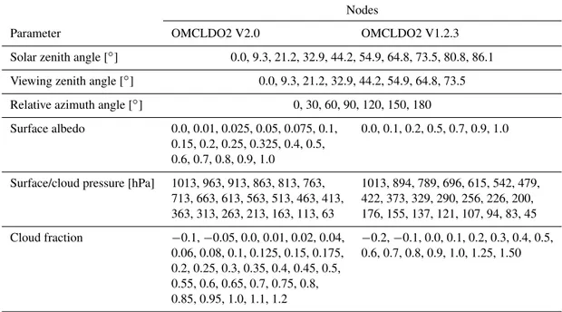
Table 1.Nodes for the radiative transfer calculations used for the OMCLDO2 algorithm v2.0 and v1.2.3. Where the nodes are the same between versions, the table cells are merged. Note that cloud fractions smaller than 0 and larger than 1 are included to enlarge the parameters space.
Nodes
Parameter OMCLDO2 V2.0 OMCLDO2 V1.2.3
Solar zenith angle [◦] 0.0, 9.3, 21.2, 32.9, 44.2, 54.9, 64.8, 73.5, 80.8, 86.1
Viewing zenith angle [◦] 0.0, 9.3, 21.2, 32.9, 44.2, 54.9, 64.8, 73.5
Relative azimuth angle [◦] 0, 30, 60, 90, 120, 150, 180
Surface albedo 0.0, 0.01, 0.025, 0.05, 0.075, 0.1, 0.0, 0.1, 0.2, 0.5, 0.7, 0.9, 1.0 0.15, 0.2, 0.25, 0.325, 0.4, 0.5,
0.6, 0.7, 0.8, 0.9, 1.0
Surface/cloud pressure [hPa] 1013, 963, 913, 863, 813, 763, 1013, 894, 789, 696, 615, 542, 479, 713, 663, 613, 563, 513, 463, 413, 422, 373, 329, 290, 256, 226, 200, 363, 313, 263, 213, 163, 113, 63 176, 155, 137, 121, 107, 94, 83, 45
Cloud fraction −0.1,−0.05, 0.0, 0.01, 0.02, 0.04, −0.2,−0.1, 0.0, 0.1, 0.2, 0.3, 0.4, 0.5, 0.06, 0.08, 0.1, 0.125, 0.15, 0.175, 0.6, 0.7, 0.8, 0.9, 1.0, 1.25, 1.50 0.2, 0.25, 0.3, 0.35, 0.4, 0.45, 0.5,
0.55, 0.6, 0.65, 0.7, 0.75, 0.8, 0.85, 0.95, 1.0, 1.1, 1.2
cf# pcld#
psfc#
Acld#
Asfc#
pscn#
Ascn#
Independent'pixel'approxima1on' Lamber1an'equivalent'reflector'
Figure 1.The independent pixel approximation versus the
Lamber-tian equivalent reflectance model. In the IPA a ground pixel is mod-elled as the weighted sum of a cloudy part, (a Lambertian surface with an albedo ofAcldat a pressure levelpsfc) and a clear part (a
Lambertian surface with an albedo ofAsfcat a pressure levelpsfc).
The top-of-atmosphere reflectance is computed as the weighted av-erage of the cloudy and clear parts, using the effective cloud frac-tioncffor the weighting. The IPA method requires knowledge on
Asfc, Acldandpsfc. In the LER model the ground pixel is modelled
as a Lambertian surface with an albedoAscnat a pressure levelpscn.
Note that the hatched areas below the opaque Lambertian indicate that these regions do not contribute in the radiative transfer calcula-tions.
For both the IPA and LER model, we use the same set of forward model simulations of the reflectance between 460 and 490 nm; see Table 1. These simulations are performed for a mid-latitude summer standard atmosphere. The correc-tion for different temperature profiles is discussed later on in this section. On the simulated reflectance the same DOAS fit is performed as for the measured OMI spectra (Eq. 1). For
all the nodes listed in Table 1, we obtain the slant column O2–O2as well as the continuum reflectance at 475 nm. The
continuum is computed by evaluating the polynomialP (λ)
for this wavelength.
2.2.2 Look-up table inversion
The radiative transfer modelling described above provides the O2–O2slant column and the continuum reflectance as a
functionf of the Sun–satellite geometry and the cloud model parameters:
Ns,O2O2=f1(θ0, θ, 1φ, cf, pcld, Asfc, psfc) , (3a)
Rc=f2(θ0, θ, 1φ, cf, pcld, Asfc, psfc) , (3b)
where Rc is the continuum reflectance, θ is the viewing
zenith angle, 1φ is the difference between the solar and viewing azimuth angles,cfis the cloud fraction,pcld is the
cloud pressure,Asfcis the surface albedo andpsfcis the
sur-face pressure. It is noted that setting the cloud fraction to 0 yields the forward model for the LER model and that the functionsf1andf2may not be fully independent.
Instead of having the slant column O2–O2and continuum
reflectance as a function of the cloud and surface parameters (Eq. 3), the retrieval requires the functionsgandhthat de-scribe the IPA and the LER model parameters as a function of the slant column O2–O2and continuum reflectance:
cf=g1 θ0, θ, 1φ, R, Ns,O2O2, Asfc, psfc
, (4a)
pcld=g2 θ0, θ, 1φ, R, Ns,O2O2, Asfc, psfc
, (4b)
Ascn=h1 θ0, θ, 1φ, R, Ns,O2O2
Table 2.Nodes for the continuum reflectance and the slant column O2–O2, for the cloud fraction/pressure and scene albedo/scene
pres-sure look-up tables. The solar zenith angle, viewing zenith angle, relative azimuth angle, surface albedo and surface/cloud pressure nodes are the same as given in Table 1.
Parameter Nodes
Continuum reflectance 0.00, 0.05, 0.10, 0.15, 0.20, 0.25,
Rcat 477 nm 0.30, 0.35, 0.40, 0.45, 0.50, 0.55,
0.60, 0.65, 0.70, 0.75, 0.80, 0.85, 0.90, 0.95, 1.00, 1.05, 1.10, 1.15, 1.20, 1.25, 1.50, 1.75, 2.00
Slant column O2–O2 0.00, 0.05, 0.10, 0.15, 0.20, 0.25, [1044molec2cm−5] 0.30, 0.35, 0.40, 0.45, 0.50, 0.55, 0.60, 0.65, 0.70, 0.75, 0.80, 0.85, 0.90, 0.95, 1.00, 1.10, 1.20
pscn=h2 θ0, θ, 1φ, R, Ns,O2O2
, (4d)
whereAscnis the scene albedo andpscnis the scene pressure.
Therefore, we invert the tables to give look-up tables with slant column O2–O2 and continuum reflectance as nodes.
This conversion process involves interpolation and extrapo-lation, for which we use linear radial basis functions (Jones et al., 2001). The inversion is illustrated in Fig. 2. Because the simulated spectra cover a very wide range of conditions, it is unlikely that the extrapolations in this inversion pro-cedure have a large effect on the final result. For example, as can be seen in the lower panel of Fig. 2, the results for the effective cloud pressure around a reflectance of 0.15 and 0.4×10−44molec2cm−5 show strange patterns due to
ex-trapolation. However, these combinations of continuum re-flectance and O2–O2slant columns will never occur for real
atmospheric conditions, and therefore these parts of the ta-bles are never reached.
The final results of the inversion procedure are LUTs for the cloud fraction, cloud pressure, scene albedo and scene pressure on the nodes listed in Table 2. In the retrieval algo-rithm linear interpolation is applied in all dimensions, except for the solar zenith angle, for which spline interpolation is applied. This is implemented because of the non-linear be-haviour at large solar zenith angles.
The previous version of the OMCLDO2 algorithms also made use of inverted LUTs. However, they were not calcu-lated using radial basis functions but computed on ad hoc fits of the continuum reflectance and slant column O2–O2
ver-sus the cloud pressure and cloud fraction. Also the number of nodes for low cloud fractions and low albedos was signif-icantly lower in the previous version.
2.2.3 Temperature correction
As will be described in this section, the slant column amount of O2–O2 depends on the temperature profile. This is not
Figure 2.Example of a slice of the effective cloud fraction LUT
(top panel) and effective cloud pressure LUT (bottom panel), show-ing the LUT value as a function of the continuum reflectanceRcand
the slant column O2–O2Ns,O2O2. The background colours show
the values in the LUT derived from interpolation and extrapolation of the DOAS fit results, which are shown as the colour-filled sym-bols. The other LUT nodes are fixed to the following values: solar zenith angle of 44.2◦, viewing zenith angle of 21.2◦, relative az-imuth angle of 0.0◦, surface albedo of 0.05 and surface altitude of 0 m.
caused by a temperature dependence of the O2–O2
absorp-tion cross secabsorp-tion but is due to the nature of the dimers, of which the abundance scales with the pressure squared instead of being linear with pressure. Because this effect turns out to be significant, we have developed a temperature correction. This correction allows the use of the LUTs described above, which have been derived for a single pressure–temperature profile. By applying temperature correction, the O2–O2slant
columns are scaled to the values for the reference tempera-ture profile that has been used to construct the LUTs.
To understand the temperature effect of the O2–O2 slant
columns, we write the reflectance as
R (λ)=R0(λ)exp
− TOA
Z
z0
m (z, λ) n2O
2(z) σO2-O2(z, λ)dz
, (5)
whereR0(λ) is the reflectance if absorption by O2–O2 is
ignored, z0 is the altitude of a Lambertian cloud or the
is the altitude-resolved air mass factor which is weakly wavelength-dependent,nO2(z)is the number density of
oxy-gen andσO2-O2(z, λ)is the absorption cross section of O2–
O2. The altitude-resolved air mass factorm (z, λ)can be
ex-pressed as
m (z, λ)= 1
R0(λ)
∂2R0(λ)
∂kabs(z, λ) ∂z. (6)
It represents the relative reduction in the reflectance when a unit amount of absorption is added to the atmosphere in a thin layer located between zandz+dz. The volume absorption coefficient is given bykabs(z, λ)=n2O
2(z) σO2-O2(z, λ).
In hydrostatic equilibrium, the integral over the altitude can be replaced by an integral over the pressure, using dp /dz= −ρ(z)g, whereρ(z)is the density of air. By ex-pressing the density of air as ρ(z)=Mp / (RgT (z)), where
M is the mean molecular mass of dry air andRgis the gas
constant, Eq. (5) becomes
R (λ)=R0(λ)exp
· pTOA Z p0 Rg
MgT (p) m (p, λ) n
2
O2(p)σO2-O2(p, λ)
dp p
. (7)
Finally, we can express the number density of air as nO2=
0.21p/(kBT (p)), wherekBis Boltzmann’s constant, and we
assume a mixing ratio of oxygen of 21 %. Substituting this in Eq. (7) gives
R (λ)=R0(λ)exp
·
(0.21)2
Rg
MgkB2σO2-O2(λ)
pTOA
Z
p0
m (p, λ) p
T (p)dp
, (8)
which shows that the reflectance and hence the slant column of O2–O2 change when the temperature profile changes. It
is noted that this is due to the density-squared nature of the absorption of O2–O2. For “normal” absorbers (no collision
complex) the slant column is independent of the temperature profile, assuming that the absorption cross section is inde-pendent of temperature and pressure.
In order to investigate the magnitude of the bias that is introduced if the temperature dependence is ignored, simu-lations of the retrieval were performed. In the retrieval the mid-latitude summer profile is used, while for the simula-tions either a mid-latitude winter profile or a subarctic win-ter profile is used. The bias was calculated for different true pressure levels of the cloud and for different cloud fractions. Figure 3 shows that the maximum bias in the retrieved cloud pressure ranges from less than 50 hPa at large cloud fractions to 200 hPa at very small cloud fractions. As discussed in the Introduction, clouds can have a shielding or an enhancing ef-fect on sensitivity of satellite measurements of trace gases. Tropospheric trace gas retrievals are commonly limited to
ground pixels with effective cloud fraction below approxi-mately 0.2–0.3, for which the cloud-free reflectance domi-nates the scene. Figure 3 shows that for these cases the bias in the cloud pressure due to the temperature effect is very large (20–200 hPa). Such biases could change the effect of the clouds as assumed in the trace gas retrieval, from shield-ing to enhancshield-ing, or vice versa, and have a significant effect on the retrieved trace gas column.
The OMCLDO2 retrieval is based on a LUT approach, and generating LUTs for many different temperature profiles is not feasible. Therefore, we introduce a correction factorγ
that translates the measured slant column into the slant col-umn for the reference pressure–temperature profile. Using Eq. (8), we can computeγ as
γ= N
ref s Nmeas s = pTOA R pcld
m (p, λ)T p
ref(p)dp
pTOA
R
pcld
m (p, λ)T (p)p dp
, (9)
where T (p) is the actual temperature profile taken and
Tref(p)is the temperature profile used in the creation of the
look-up tables. In the case of partial cloud cover and weak absorption we obtain
γ= N
ref s
Nsmeas (10)
=
(1−cf) Rclr
pTOA
R
psfc
mclr(p, λ)Trefp(p)dp+cfRcld
pTOA
R
pcld
mcld(p, λ)Trefp(p)dp
(1−cf) Rclr
pTOA
R
psfc
mclr(p, λ)T (p)p dp+cfRcld
pTOA
R
pcld
mcld(p, λ)T (p)p dp
,
whereRis the reflectance at a representative wavelength in the fit window;psfcis the surface pressure andpcldthe cloud
pressure; and the subscripts clr and cld refer to the clear part and the cloudy part of the pixel, respectively.
To implement the temperature correction factor, new look-up tables for the O2–O2air mass factorsm(p, λ)and the
cor-responding reflectance for a wavelength in the middle of the fit window have been generated. In the retrieval algorithm, the temperature correction is applied in an iterative manner because the cloud fraction and pressure should be known to computeγ. As a default, we use three iterations to compute
γ.
2.2.4 Input data
The OMCLDO2 version 2 uses the following input. For the absorption cross sections for O2–O2, ozone and optionally
NO2, as well as for the radiance Raman scattering, we use
Table 3.Impact of the improvements of the effective cloud fraction and effective cloud pressure retrievals.
Improvement Impact onpcld Impact oncf
Temperature Decreasing at higher latitudes Negligible correction Increasing in the tropics and sub-tropics
1pcld:−100 to 150 hPa forcf< 0.2
1pcld:−20 to 40 hPa forcf> 0.2
New look-up Impact is non-significant forcf> 0.3 1cf:−0.01 except for tables 1pcld:−60 to 220 hPa forcf< 0.3 high surface reflectivity,
for which1cf> 0.05
Outlier removal No systematic impact Negligible
Digital elevation Impact restricted to mountainous terrain Negligible model 1pcldfor most pixels smaller than±25 hPa
Cross sections 1pcld: 23±23 hPa Negligible
0 50 100 150 200
0 0.2 0.4 0.6 0.8 1
Lambertian cloud fraction
p_r
et
r
-
p_t
rue
300 hPa mlw
500 hPa mlw
700 hPa mlw
800 hPa mlw
300 hPa saw
800 hPa saw
Figure 3.Bias in the retrieved pressure (pretr−ptrue) in hPa when
in the retrieval a mid-latitude summer temperature profile is used, whereas in the simulation a mid-latitude winter profile (mlw) or a subarctic winter profile (saw) is used. The results are plotted as a function of the cloud fraction and for different pressure levels of the cloud used in the simulation. The surface albedo is fixed at 0.05, the cloud albedo is 0.80, the solar zenith angle is 60◦and the viewing direction is nadir.
(00:00, 06:00, 12:00 and 18:00 UTC), derived from the Na-tion Centers for Environmental PredicNa-tion (NCEP) reanaly-sis data for the period 2005–2014. Actual temperatures will be somewhat better than using a climatology. However, for practical reasons related to the operational data processing facility, we have decided to use a temperature climatology. For detecting snow and sea-ice coverage, the Near-real-time Ice and Snow Extent (NISE) product (Nolin et al., 1998) is used.
3 Impact of algorithm updates
In this section we first compare the OMCLDO2 version 2 with version 1.2.3 for 1 day of data. Next, the impacts of each of the improvements are discussed separately. The impacts of the improvements are summarized in Table 3.
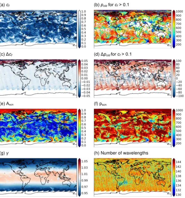
Figure 4 shows the OMCLDO2 retrieval results for 14 May 2005. This day has been selected arbitrarily from the OMI data record. Note that we also have analysed other days, which show consistent results. Figure 4a and b show the ef-fective cloud fraction and the efef-fective cloud pressure. Fig-ure 4c and d show the difference between versions 2 and 1.2.3. For areas with low effective cloud fractions, the effec-tive cloud fraction is approximately 0.01 larger in version 2. Over the high latitudes in the Northern Hemisphere consid-erably large positive and negative differences occur. These occur over snow and ice, where the retrieval algorithm has problems distinguishing the clouds from the highly reflective surface. Under such conditions, the accuracy of the retrieved effective cloud fraction will be very low. Due to the assumed cloud albedo of 0.8, the cloud fraction will become undeter-mined when the surface albedo is close to this value.
illus-(a) cf (b) pcld for cf> 0.1
(c) Δcf (d) Δpcld for cf> 0.1
(e) Ascn (f) pscn
(g) γ (h) Number of wavelengths
Figure 4.Results from the OMCLDO2 version 2 algorithm for 14 May 2005.(a)Effective cloud fraction,(b)effective cloud pressure,
(c)difference of the effective cloud fraction (version 1.2.3 minus version 2),(d)difference of the effective cloud pressure (version 1.2.3 minus version 2),(e)scene albedo,(f)scene pressure,(g)temperature correction factorγand(h)number of wavelengths used in the DOAS fit.
trated in Fig. 5, which shows the precision of the effective cloud pressure retrievals as a function of the effective cloud pressure. The precision is calculated by the propagation of the DOAS fit errors of the O2–O2slant columns and of the
continuum reflectance. For cloud fractions below 0.1 the av-erage precision is larger than 20 hPa with a very large spread, whereas for cloud fractions above 0.9 the precision is less than 10 hPa with a much smaller spread. It is noted that other errors sources, for example in the assumed surface albedo, will also have a much stronger impact at low effective cloud fractions.
3.1 Temperature correction
The correction for the temperature dependence is described above. Based on a temperature climatology, a correction fac-tor is computed and applied to the O2–O2 slant columns.
0.05 0.15 0.25 0.35 0.45 0.55 0.65 0.75 0.85 0.95 Effective cloud fraction [unitless]
0 20 40 60 80 100 120
Precision of the effective cloud pressure [hPa]
2005-05-14
Figure 5. Box-and-whisker plot of the precision of the effective
cloud pressure as a function of the effective cloud fraction for 14 May 2005.
and thick clouds, the temperature correction is in most cases closer to 1, indicating that the largest differences between the climatological temperature and the mid-latitude summer at-mosphere occur at the lowest altitudes.
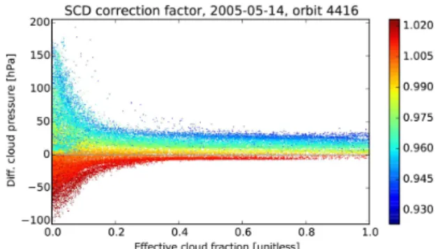
To test the impact of the temperature correction factor on the effective cloud fraction and pressure, we produced datasets with and without the temperature correction applied for 2 days of OMI data in different seasons (14 May and 15 November 2005). While the impact on the cloud fraction is negligible, the impact on the cloud pressure can be signif-icant. Figure 6 shows the difference between the retrievals without and with the correction applied, as a function of the effective cloud fraction. The impact of the correction on the cloud pressure increases towards smaller cloud fractions. De-pending on whether the correction factor is smaller or larger than 1, the impact on the cloud pressure can be both positive or negative. For cloud fractions below 0.2, the impact of the temperature correction can be as large as −100 to 150 hPa, whereas for cloud fractions larger than 0.2 the impact is in the range−20 to 40 hPa. For the higher latitudes (γ< 1) the clouds are at lower pressures (higher altitude) when the tem-perature correction is applied, whereas in the tropics and sub-tropics the effects are reversed.
Figure 6 can be compared to Fig. 3, which is based on retrieval simulations. Although Fig. 6 shows the difference with and without the temperature corrections, and Fig. 3 shows the difference with the simulated truth, the behaviour and magnitude of the bias are very similar. It is noted that for Fig. 3 only temperature profiles have been used which are colder in the troposphere than the reference mid-latitude summer atmosphere. Therefore, Fig. 3 shows only positive biases, whereas in the tropics and sub-tropics Fig. 6 also shows negative values.
Figure 6.Difference in the effective cloud pressure due to the
tem-perature correction (without correction minus with correction) plot-ted as a function of the effective cloud fraction. The colours of the symbols indicate the temperature correction factorγ.
3.2 Look-up tables
To test the impact of the LUTs that are used to derive the effective cloud fraction and effective cloud pressure, we pro-duced datasets using version 2 algorithm with the new and the old LUTs. The cloud fraction with the new LUTs is about 0.01 larger than with the old version, except over snow and ice regions, where the cloud fraction with the new LUT is in most cases significantly smaller. Because over snow- and ice-covered regions the cloud fraction is highly uncertain as the algorithm is not able to distinguish clouds from highly reflective surfaces, this impact is not unexpected.
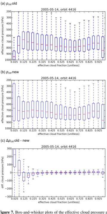
The effect of the new LUTs on the effective cloud pressure is shown in Fig. 7c. This figure shows the difference in the cloud pressure (old minus new) as a function of the effective cloud pressure. The differences become significant at cloud fractions smaller than 0.25, where the difference shows an oscillating behaviour. At acfof approximately 0.125 a
mini-mum is reached, and at smaller cloud fractions the mean dif-ference reverses sign and increases towards lowercf. To
in-vestigate the nature of this behaviour, Fig. 7a and b show the distribution of the retrieved cloud pressures as a function of cloud fraction for the old and new LUT datasets. From these figures it is clear that the origin of the oscillating behaviour of the difference is in the retrievals with the old LUTs. Fig-ure 7a shows that with the old LUTs the cloud pressFig-ure in-creases strongly towards lower cloud fractions, for which we have no physical explanation. The results with the new LUTs (Fig. 7b) do not show this. We attribute the large improve-ments with the new LUTs to the larger number of radiative transfer calculations on which it is based (see Table 1), as well as the improved interpolation scheme that was used to produce it.
Figure 7a and b also show that the effective cloud pressure for the largestcfbin is significantly larger. A further
a)
( pcldold
b)
( pcldnew
c)
( Δpcldold - new
Figure 7.Box-and-whisker plots of the effective cloud pressure as
a function of the effective cloud fraction. The top plot is for the old LUTs, the middle for the new LUTs and the bottom plot for the difference of old minus new.
are highly uncertain. For such cases the scene albedo and pressure provided by version 2 of the algorithm can be used. 3.3 Outlier removal
The outlier removal procedure that was introduced in ver-sion 2 of the algorithm removes spectral pixels from the DOAS fit after evaluation of the fitting residuals. Outliers can have different behaviour: they can be transient, e.g. oc-curring only for spectral pixels for a few pixels, or they can occur systematically for certain spectral pixels. When
out-liers are detected, they are removed from the data, which will decrease the number of wavelengths used in the DOAS fit. Figure 4h shows the number of wavelengths used in the fit for 14 May 2005. The most prominent feature is the re-duced values over South America caused by the South At-lantic Anomaly (SAA). In this region the number of high en-ergetic particles hitting the OMI detectors is significantly in-creased (Dobber et al., 2006), resulting in spikes in the data. It is noted that also the Level 0–1B processor flags transient pixels, so Fig. 4h is the result of the Level 1B flags in com-bination with the outlier removal procedure. In addition to the SAA, Fig. 4h also shows stripes in the along-track direc-tion, as well as features related to geophysical conditions (for example higher values for Australia and India).
The impact of the outlier removal procedure was tested by running the algorithm with and without the procedure switched on for 14 May 2005. The differences in the re-trieved effective cloud fraction are negligible, whereas the impact on the effective cloud pressure depends on the cloud fraction. The mean difference is not significant, but the standard deviation of the difference varies from 16 hPa for
cf< 0.2 to 3 hPa forcf< 0.8.
We also inspected the root-mean-square error (RMSE) of the DOAS fit as a fit quality indicator. Although the differ-ence in RMSE with and without the outlier removal did not differ significantly from 0, the distribution is skewed towards larger RMSE values when the outlier removal is switched off. This indicates that the outlier removal procedure improves the fit for cases with a high RMSE.
3.4 Digital elevation model (DEM)
Version 2 of the algorithm uses a DEM with a resolution of approximately 20 km, which is closer to the spatial reso-lution of OMI compared to the 3 km resoreso-lution DEM used in previous versions. The 20 km resolution DEM is con-structed from the Global Multi-resolution Terrain Elevation Data 2010 (Danielson and Gesch, 2011).
The impact of the new DEM will be largest in mountain-ous terrain. Figure 8 illustrates the effect on the retrieved ef-fective cloud pressures over Europe for 14 May 2005. This is the same day as shown in Fig. 4. Figure 8a shows that sig-nificant impacts of the new DEM are restricted to the main mountain ranges. The difference between using the old and new DEM can be both positive and negative. The impact in-creases towards the lower cloud fractions, when more signal comes from the surface and an accurate knowledge of the surface altitude becomes more important. Figure 8b shows that for most pixels the impact is smaller than±50 hPa. 3.5 Cross sections
Figure 8.Difference in the effective cloud pressure (old DEM minus new DEM) for effective cloud fractions exceeding 0.1 over Europe for 14 May 2005. Left panel: map of the differences over Europe; right panel: histogram of the differences over Europe on a logarithmic scale.
with the old and the new cross sections. The impact on the cloud fraction was negligible. Using the new cross sections increased the effective cloud pressures by 23±23 hPa. The difference in the root-mean-square error of the DOAS was not significant. The new cross sections did not significantly reduce the residuals of the DOAS fit.
3.6 Scene albedo and scene pressure
As described in the algorithm section, for each ground pixel the scene albedo and scene pressure are derived. The most important application of these parameters is over bright sur-faces such as snow and ice, where the surface albedo be-comes close to the assumed cloud albedo of 0.8 and no mean-ingful cloud fraction and pressure can be derived. Figure 9 shows a comparison of the retrieved scene pressure with the surface pressure derived from the DEM, assuming a sea level pressure of 1013 hPa. The figure shows a very good agree-ment between the retrieved scene pressure and the DEM over Greenland. This figure presents the comparison for the OMI cross-track pixel 20, but other cross-track pixels show similar results. It demonstrates the capabilities of the scene pressure for bright surfaces. Also, it is an indirect validation of the retrieved O2–O2slant columns. A correction of the O2–O2
slant columns, as is sometimes used in ground-based DOAS measurements (for a discussion see Spinei et al., 2015), is clearly not necessary for the OMCLDO2 retrievals.
Over dark scenes, such as over oceans under conditions with low cloud fractions, the scene pressure is less well un-derstood. For some areas over the ocean the retrieved scene pressure is significantly larger than the sea level pressure. For scene albedos of less than 5 %, about 3 % of the scene pres-sures exceed 1050 hPa, and 50 % exceed 1013 hPa. We note that scene pressures larger than 1013 hPa are the results of ex-trapolation and therefore should be used with great caution. For dark scenes we recommend using the cloud fraction and cloud pressure, taking into account that there will be a large uncertainty in the cloud pressure in these cases (see Fig. 5).
Figure 9.Top panel: map of the position of the ground pixel centres.
Bottom panel: comparison of the retrieved scene pressure and the surface pressure derived from the DEM, plotted as a function of the longitude.
4 Comparison with ground-based radar–lidar observations
pos-sible to compare the same quantity, which is required in a validation study. Rather than conducting a validation study, we focus on explaining the differences between the OMI re-trievals and the radar–lidar data, given their different sensitiv-ities. This comparison uses a similar approach to that used for comparing Scanning Imaging Absorption Spectrometer for Atmospheric CHartographY (SCIAMACHY) cloud products with radar–lidar data (Wang and Stammes, 2014).
We present comparisons for three sites: Cabauw, the Netherlands; Lindenberg, German; and the Atmospheric Ra-diation Measurement (ARM) Southern Great Plains (SGP), USA, for the period January to June 2005. These datasets were selected because of the continuous data availability for these sites in the Cloudnet (Illingworth et al., 2007) database. Cloudnet is a network of stations for the continuous evalua-tion of cloud and aerosol profiles.
4.1 Cloudnet data
We use the Cloudnet Level 2 classification product (Illing-worth et al., 2007), which is based on the combination of Radar and Lidar observations and is available approximately every 30 s. This product classifies each vertical layer as 1 of 11 classes, which distinguish ice and water clouds, precipi-tation, aerosols, insects, clear sky and combinations thereof. We attribute a value of 1 to layers that are classified as cloudy (classes 1–7) and 0 to layers identified as non-cloudy. For profiles containing at least one cloudy layer, we compute the cloud mid-height as the average of the altitude of the cloudy layers. Next we average all the profiles in the time window of
±30 min of an OMI overpass. We also compute the average and standard deviation of the cloud mid-height over this time window and determine for the average cloud profile if it is single layer or multi-layer.
It is noted that this procedure for computing the cloud mid-height does not take the optical thickness of the layers into account; an optically thick cloud and optically thin cloud are weighted the same in the cloud mid-height. Weighting with the optical thickness – or even better, with the sensitiv-ity of the O2–O2cloud algorithm – would make a
compari-son much more direct. Unfortunately, information on the full optical thickness profile is not available from the Cloudnet data. Alternatively, we could use the Radar reflectivity as a weighting parameter. However, the Radar reflectivity is very sensitive to cloud particle size, which is also not a good rep-resentation for the cloud extinction in the visible. We there-fore decided to use the simple weighting described above. This weighting gives the same weight to optically thin cloud layer as to optically thick layers, whereas the O2–O2 cloud
pressure retrieval is much more sensitive to the thick layers. Further filtering of the Cloudnet data was done using the following criteria:
– the standard deviation of the cloud mid-height should not exceed 1.5 km, to avoid cases with large temporal variability during the OMI overpass;
0 20 40 60 80 100 120
Case no.
0 2 4 6 8 10 12
Cloud altitude [km]
abauw; 135 points Cloudnet
OMI
0.0 0.1 0.2 0.3 0.4 0.5 0.6 0.7 0.8 0.9 1.0
C
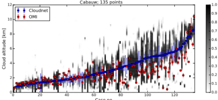
Figure 10.The effective cloud altitude retrieved from OMI (red),
compared to radar–lidar cloud information for Cabauw (blue), the Netherlands. The grey background is the vertically resolved cloud occurrence derived from the radar–lidar data for the period±30 min of the OMI overpass. The cases are ordered according to the ground station cloud mid-height.
– at least one layer in the profile should be cloudy during at least 50 % of the time averaging window.
4.2 OMI collocated data
For the OMI cloud data, we average all the ground pixels of which the centre is within 30 km distance of the ground station. For these pixels we determine the mean and standard deviation for the cloud fraction and pressure. We convert the cloud pressure to altitude using a scaling height of 8 km. We filter the OMI data using the following criteria:
– the effective cloud fraction should exceed 0.2, because the cloud pressure for low cloud fraction has a large un-certainty;
– the standard deviation of effective cloud pressures should not exceed 1.5 km, to exclude cases with large horizontal variability.
4.3 Results
Figure 10 shows a comparison between the Cloudnet data and the OMI effective cloud pressure for the collocations over Cabauw for the period January to June 2005. The cases presented in this figure are ordered by increasing mid-height of ground-based data. The following regimes can be distin-guished in this dataset:
1. Case 1–50: these are low level clouds with limited ver-tical extent. The OMI effective cloud height and the ground station mid-height are in good agreement. 2. Case 51–129: according to Cloudnet the majority of
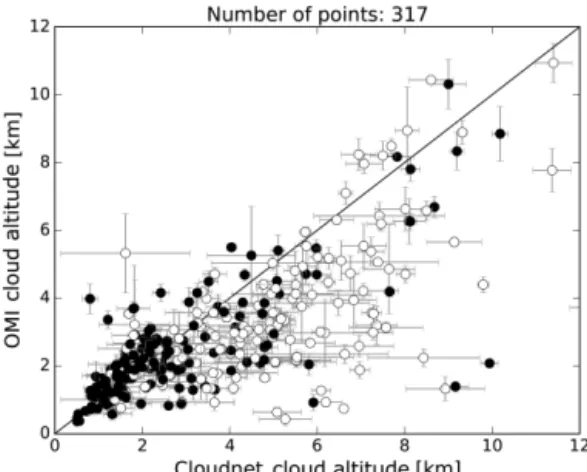
Figure 11.The retrieved effective cloud altitude from OMI, plotted as a function of the radar–lidar-derived cloud altitude. Closed sym-bols are for single-layer clouds; open symsym-bols are for multi-layer clouds.
3. Case 130–135: these cases have high clouds with lim-ited vertical extent. The OMI effective cloud height compares well, except for the outlier for case 131. How-ever, the number of collocations in this regime is small. It is noted that the boundaries of these three regimes are not hard.
Figure 10 shows that for single layer clouds with a lim-ited vertical extent the O2–O2effective cloud height and the
Cloudnet-derived mid-height are in agreement. This shows that the OMI-derived product is capable of retrieving cloud height ranging from low clouds to high clouds. For vertically extended clouds, the OMI-derived cloud heights are gener-ally lower than the radar–lidar-derived heights. A plausible explanation for this difference is that in these cases there are thin high clouds overlaying thicker low-level water clouds. Whereas the radar–lidar mid-heights have equal sensitivity, the O2–O2cloud height will be more sensitive to the
opti-cally thick layers at lower altitude.
When we include not only Cabauw but also Lindenberg and the ARM-SGP site, we get a similar picture. Figure 11 shows a comparison for all these sites for the period January– June 2005, where the single- and multi-layer cloud cases are distinguished. Good correlation is observed for the cloud range of 0–2.5 km, where the single cloud layers dominate. In the region between 2.5 and approximately 8 km the multi-layer clouds dominate and the O2–O2cloud height is lower
than the radar–lidar cloud mid-height. Above 8 km we find both good comparison and very large differences, although the number of points is very limited. As we are interested in the average comparisons, we did not investigate individual cases where big differences occurred.
The comparison between the Cloudnet data was repeated for the old version of the OMCLDO2 algorithm. The results were very similar to those presented in Figs. 10 and 11. This is expected because for effective cloud fractions larger than
20 % the difference between the old and the new algorithm is not very large. Moreover, the difference between the two al-gorithm versions is smaller than with the ground-based data, because of the different sensitivity of ground-based versus satellite observations and because of representation errors in both space and time.
5 Conclusions
We present a new version of the OMI OMCLDO2 Level 2 cloud product. This product is an important input for sev-eral of the operational OMI Level 2 algorithms. The new ver-sion contains six major improvements:
1. the correction for the temperature sensitivity of the DOAS fit;
2. improved look-up tables for computing the effective cloud fraction and effective cloud pressure;
3. retrieval of the scene pressure and scene albedo for ev-ery ground pixel, using the Lambertian equivalent re-flectance model;
4. outlier removal procedure in the DOAS fit. 5. updated gas absorption cross sections;
6. introduction of a DEM with a similar resolution as the OMI ground pixels.
We show that the impact of these changes on the retrieved effective cloud fraction is for most ground pixels less than 0.01. The impact on the effective cloud pressure is larger: es-pecially for cloud fractions less than approximately 0.3 the differences compared to the previous operational version can be as large as 200 hPa. These differences are mainly caused by the temperature correction and the introduction of the new look-up tables. Due to the temperature the differences have a latitudinally and seasonally dependent behaviour, where the updated algorithm gives higher cloud pressures at higher lati-tudes and lower pressures in the tropics and sub-tropics. Also it was found that the new look-up tables give better results at low cloud fractions.
We conclude that the new version of the OMCLDO2 prod-uct is a significant improvement of the previous versions, especially for the cloud pressure at cloud fractions smaller than approximately 0.3. This is very important for cloud cor-rections in retrievals of gases like nitrogen dioxide, sulphur dioxide and formaldehyde, which are very sensitive to the cloud pressure.
After reprocessing of the entire OMI data record, the sta-bility of the product should be investigated, and the scene pressure and scene albedo should be validated.
6 Data availability
The OMCLDO2 dataset is available from the NASA archives: https://disc.gsfc.nasa.gov/uui/datasets/ OMCLDO2_003/summary. DOI provided by NASA is doi:10.5067/Aura/OMI/DATA2007.
Acknowledgements. This work was funded by the Netherlands Space Office under the OMI Science Contract.
We acknowledge the EU Cloudnet and the ACTRIS (European Research Infrastructure for the observation of Aerosol, Clouds, and Trace gases) projects for providing the cloud classification datasets for the Cabauw, Lindenberg and the ARM-SGP sites. We thank Phil Durbin and his team for the processing of the various versions of the OMCLDO2 algorithm. We also thank two anonymous reviewers for their important and constructive comments.
Edited by: N. Kramarova
Reviewed by: two anonymous referees
References
Acarreta, J. R., De Haan, J. F., and Stammes, P.: Cloud pressure retrieval using the O2-O2absorption band at 477 nm, J. Geophys. Res., 109, D05204, doi:10.1029/2003JD003915, 2004.
Boersma, K. F., Eskes, H. J., and Brinksma, E. J.: Error analysis for tropospheric NO2retrieval from space, J. Geophys. Res., 109,
D04311, doi:10.1029/2003JD003962, 2004.
Boersma, K. F., Eskes, H. J., Dirksen, R. J., van der A, R. J., Veefkind, J. P., Stammes, P., Huijnen, V., Kleipool, Q. L., Sneep, M., Claas, J., Leitão, J., Richter, A., Zhou, Y., and Brunner, D.: An improved tropospheric NO2column retrieval algorithm for
the Ozone Monitoring Instrument, Atmos. Meas. Tech., 4, 1905– 1928, doi:10.5194/amt-4-1905-2011, 2011.
Bogumil, K., Orphal, J., and Burrows, J. P.: Temperature dependent absorption cross sections of O3, NO2, and other atmospheric
trace gases measured with the SCIAMACHY spectrometer, in Looking down to Earth in the New Millennium, vol. SP-461, Gothenburg, 2000.
Burrows, J., Vountas, M., Haug, H., Chance, K., Marquard, L., Muirhead, K., Platt, U., Richter, A., and Rozanov, V.: Study of the Ring effect, Tech. Rep. ESA contract 10996/94/NL/CN, Eur. Space Agency, Noordwijk, Netherlands, 1996.
Chance, K. V. and Spurr, R. J. D.: Ring effect studies: Rayleigh scattering, including molecular parameters for rotational Raman scattering, and the Fraunhofer spectrum, Appl. Opt., 36, 5224– 5230, 1997.
Danielson, J. J. and Gesch, D. B.: Global Multi-resolution Ter-rain Elevation Data 2010 (GMTED2010), US Geological Survey, available at: http://topotools.cr.usgs.gov/gmted_viewer/ (last ac-cess: 12 December 2016), 2011.
Dobber, M., Voors, R., Dirksen, R., Kleipool, Q., and Levelt, P.: The High-Resolution Solar Reference Spectrum between 250 and 550 nm and its Application to Measurements with the Ozone Monitoring Instrument, Sol. Phys., 249, 281–291, doi:10.1007/s11207-008-9187-7, 2008.
Dobber, M. R., Dirksen, R. J., Levelt, P. F., Van Den Oord, G. H. J., Voors, R. H., Kleipool, Q., Jaross, G., Kowalewski, M., Hilsenrath, E., Leppelmeier, G. W., de Vries, J., Dierssen, W., and Rozemeijer, N. C.: Ozone monitoring instrument calibration, Geosci. Remote Sens., 44, 1209–1238, 2006.
Illingworth, A. J., Hogan, R. J., O’Connor, E. J., Bouniol, D., De-lanoë, J., Pelon, J., Protat, A., Brooks, M. E., Gaussiat, N., Wil-son, D. R., Donovan, D. P., Baltink, H. K., van Zadelhoff, G.-J., Eastment, J. D., Goddard, J. W. F., Wrench, C. L., Haeffelin, M., Krasnov, O. A., Russchenberg, H. W. J., Piriou, J.-M., Vinit, F., Seifert, A., Tompkins, A. M., and Willén, U.: Cloudnet, B. Am. Meteor. Soc., 88, 883–898, doi:10.1175/BAMS-88-6-883, 2007. Joiner, J. and Vassilkov, A. P.: First Results From the OMI Rota-tional Raman Scattering Cloud Pressure Algorithm, T. Geosci. Remote, 44, 1272–1282, doi:10.1109/TGRS.2005.861385, 2006. Joiner, J., Vasilkov, A. P., Gupta, P., Bhartia, P. K., Veefkind, P., Sneep, M., de Haan, J., Polonsky, I., and Spurr, R.: Fast simula-tors for satellite cloud optical centroid pressure retrievals; evalu-ation of OMI cloud retrievals, Atmos. Meas. Tech., 5, 529–545, doi:10.5194/amt-5-529-2012, 2012.
Jones, E., Oliphant, T., Peterson, P., and others: SciPy: Open source scientific tools for Python, available at: http://www.scipy.org/ (last access: 12 December 2016), 2001.
Kleipool, Q. L., Dobber, M. R., de Haan, J. F., and Levelt, P. F.: Earth surface reflectance climatology from 3 years of OMI data, J. Geophys. Res., 113, D18308, doi:10.1029/2008JD010290, 2008.
Levelt, P. F., van den Oord, G. H., Dobber, M. R., Malkki, A., Visser, H., de Vries, J., Stammes, P., Lundell, J. O., and Saari, H.: The ozone monitoring instrument, T. Geosci. Remote, 44, 1093–1101, 2006.
Nolin, A., Armstrong, R., and Maslanik, J.: Near-Real-Time SSM/I-SSMIS EASE-Grid Daily Global Ice Concentration and Snow Extent, Version 4, NASA National Snow and Ice Data Cen-ter Distributed Active Archive CenCen-ter, Boulder, Colorado, USA, available at: http://dx.doi.org/10.5067/VF7QO90IHZ99 (last ac-cess: 9 December 2016), 1998.
Richter, A., Begoin, M., Hilboll, A., and Burrows, J. P.: An im-proved NO2retrieval for the GOME-2 satellite instrument,
At-mos. Meas. Tech., 4, 1147–1159, doi:10.5194/amt-4-1147-2011, 2011.
Spinei, E., Cede, A., Herman, J., Mount, G. H., Eloranta, E., Mor-ley, B., Baidar, S., Dix, B., Ortega, I., Koenig, T., and Volkamer, R.: Ground-based direct-sun DOAS and airborne MAX-DOAS measurements of the collision-induced oxygen complex, O2O2,
absorption with significant pressure and temperature differences, Atmos. Meas. Tech., 8, 793–809, doi:10.5194/amt-8-793-2015, 2015.
Stammes, P., Sneep, M., de Haan, J. F., Veefkind, J. P., Wang, P., and Levelt, P. F.: Effective cloud fractions from the Ozone Moni-toring Instrument: Theoretical framework and validation, J. Geo-phys. Res., 113, D16S38, doi:10.1029/2007JD008820, 2008. Thalman, R. and Volkamer, R.: Temperature dependent absorption
cross-sections of O2-O2collision pairs between 340 and 630 nm
and at atmospherically relevant pressure, Phys. Chem. Chem. Phys., 15, 15371–15381, doi:10.1039/C3CP50968K, 2013. van Geffen, J. H. G. M., Boersma, K. F., Van Roozendael, M.,
Hen-drick, F., Mahieu, E., De Smedt, I., Sneep, M., and Veefkind, J. P.: Improved spectral fitting of nitrogen dioxide from OMI in the 405–465 nm window, Atmos. Meas. Tech., 8, 1685–1699, doi:10.5194/amt-8-1685-2015, 2015.
Voors, R., Dobber, M., Dirksen, R., and Levelt, P.: Method of cali-bration to correct for cloud-induced wavelength shifts in the Aura satellite’s Ozone Monitoring Instrument, Appl. Opt., 45, 3652– 3658, doi:10.1364/AO.45.003652, 2006.
Wang, P. and Stammes, P.: Evaluation of SCIAMACHY Oxygen A band cloud heights using Cloudnet measurements, Atmos. Meas. Tech., 7, 1331–1350, doi:10.5194/amt-7-1331-2014, 2014. Wang, P., Stammes, P., van der A, R., Pinardi, G., and van
Roozen-dael, M.: FRESCO+: an improved O2 A-band cloud retrieval
algorithm for tropospheric trace gas retrievals, Atmos. Chem. Phys., 8, 6565–6576, doi:10.5194/acp-8-6565-2008, 2008. Zuidema, P. and Evans, K. F.: On the validity of the