www.nat-hazards-earth-syst-sci.net/10/1851/2010/ doi:10.5194/nhess-10-1851-2010
© Author(s) 2010. CC Attribution 3.0 License.
and Earth
System Sciences
GIS and statistical analysis for landslide susceptibility mapping
in the Daunia area, Italy
F. Mancini, C. Ceppi, and G. Ritrovato
Department of Architecture and Urban Planning, Technical University of Bari, Bari, Italy
Received: 25 January 2010 – Revised: 9 June 2010 – Accepted: 16 July 2010 – Published: 7 September 2010
Abstract. This study focuses on landslide susceptibility mapping in the Daunia area (Apulian Apennines, Italy) and achieves this by using a multivariate statistical method and data processing in a Geographical Information System (GIS). The Logistic Regression (hereafter LR) method was chosen to produce a susceptibility map over an area of 130 000 ha where small settlements are historically threatened by land-slide phenomena. By means of LR analysis, the tendency to landslide occurrences was, therefore, assessed by relating a landslide inventory (dependent variable) to a series of causal factors (independent variables) which were managed in the GIS, while the statistical analyses were performed by means of the SPSS (Statistical Package for the Social Sciences) soft-ware. The LR analysis produced a reliable susceptibility map of the investigated area and the probability level of landslide occurrence was ranked in four classes. The overall perfor-mance achieved by the LR analysis was assessed by local comparison between the expected susceptibility and an in-dependent dataset extrapolated from the landslide inventory. Of the samples classified as susceptible to landslide occur-rences, 85% correspond to areas where landslide phenom-ena have actually occurred. In addition, the consideration of the regression coefficients provided by the analysis demon-strated that a major role is played by the “land cover” and “lithology” causal factors in determining the occurrence and distribution of landslide phenomena in the Apulian Apen-nines.
1 Introduction
This study applied the multivariate statistical Logistic Re-gression (LR) method to achieve landslide susceptibility mapping in the Daunia Mts. sector, the Apulian portion of
Correspondence to:F. Mancini ([email protected])
the Italian Apennines chain. This area is historically threat-ened by slope failure phenomena (Cotecchia, 1963; Iovine et al., 1996; Zezza et al., 1994) but a comprehensive investiga-tion of the proneness to landslide phenomena of the Daunia Mts. territory has not previously been performed.
The study area covers 130 000 ha and includes 25 small municipalities belonging to the administrative district of Fog-gia (Fig. 1). It is characterised by hilly terrains, that reach a maximum altitude of 1143 m a.s.l., and small urban areas that are sometimes located on steep slopes.
The geological setting of the Daunia region originated from the evolution of the Apennine chain, a Neogene and Quaternary thrust belt within the central Mediterranean oro-genic system. Being a part of the whole chain, the South-ern Apennines are made of a stack of Meso-Cenozoic tec-tonic units covered by marine turbiditic sedimentary de-posits of the Quaternary period. The deposits consist of limestone and/or sandstone layers interbedded with clay-like marls, clays and silty-clays. Effects due to more recent tec-tonic events have since modified the original sedimentary set-up and the sedimentary successions have been found to be affected by different fissuring intensities (Cotecchia et al., 2009).
1
Fig. 1.Location map showing the administrative boundaries of the 25 small municipalities threatened by slope failure (Daunia Mts., Italian Apennines, Apulian sector).
the location and distribution of landslides in a single map is a difficult task due to the geographical extension of the area and the large number of recorded landslides, but some photographs of a few significant phenomena that occurred at Volturino (FG) are shown in Fig. 2.
Among the variety of existing statistical techniques for data processing of geographical information, the LR was chosen to produce a susceptibility map over the area. By LR, a best fit between the presence or absence of a land-slide (dependent variable) and a set of possible causal fac-tors (independent variables) is established on the basis of a maximum likelihood criterion, and yields an estimation of regression coefficients that are representative of the relation-ship between the factors and the phenomena. The reliability of such an analysis is, therefore, related to its ability to iden-tify the proneness to landslide occurrences and to establish a ranking of landslide susceptibility.
The basic properties of LR analysis will be introduced in the next section, but it must be borne in mind that a range of alternative methods for preparing landslide susceptibility
1
map is currently available in the literature. In Ayalew et al. (2005a) an interesting summary of the most commonly used methods for landslide susceptibility analysis can be found, together with a complete reference list. Relevant stud-ies have also been proposed by Lee and Sambath (2006), who compared the use of frequency ratio and LR models, Lee et al. (2007), who added studies related to the use of artificial neural networks and Akgun et al. (2008), where the likeli-hood of frequency ratio and a weighted linear combination model are compared. Recently, Ayalew et al. (2005b) intro-duced the use of a couple of methods for landslide suscep-tibility mapping: the first using bivariate statistical analysis to classify quantitative variables and the second, based on the Analytic Hierarchy Process (AHP), to assign weights to the attributes. More recently, interesting papers proposed by the B. Pradhan and co-authors research group, based on back propagation ANN and fuzzy algorithms, are worthy of note as the latest results in this discipline (Pradhan et al., 2009; Pradhan and Lee, 2010a, b).
Some of the causal factors adopted are derived from a DEM (Digital Elevation Model), which must meet minimum requirements in terms of spatial resolution and vertical ac-curacy with respect to the scale of investigation and the ex-pected reliability of other, DEM-derived variables. Causal factors based on elevation data are very often cited as “mor-phometric variables” and, among these, the following will be adopted in the present study: altitude, slope angle, slope exposure, planform curvature and profile curvature. How-ever, the most promising techniques in assessing the prone-ness to slope failure (hereafter called susceptibility) at a re-gional scale rely on statistical methods that require, in addi-tion, large amounts of non-morphometric information to de-scribe variables in the geographical and geological domains. Drainage capacity, lithology, land coverage and the presence of water sources or roads could constitute a possible set of non-morphometric causal factors. Nevertheless, an inventory of existing landslides has to be created, within the investi-gated area, in order to determine the relationship between the presence/absence of landslides and the geographical dataset representing possible causal factors. To identify such rela-tionships, the Logistic Regression approach is particularly suitable when the variables involved do not follow random distributions and factors are not necessarily related to the phenomenon by a linear function (Menard, 2001). A calcula-tion of the factors and management of the landslide inventory requires the use of a GIS working environment and, there-fore, the creation of an appropriate geodatabase where vector and raster data are properly defined. As already pointed out, the capacity to perform the data analysis discussed in this paper is not a common tool within the most widely avail-able GIS packages and a reliavail-able statistical software package (SPSS in this work) is, therefore, required.
The management within the GIS environment of variables representing potential causal factors and the final suscepti-bility map provided by the Logistic Regression analysis are
examined in this paper, paying particular attention to the de-scription of the causal factors analysed, the overall perfor-mance achieved by the analysis, as verified using validation procedures, and a discussion of the relevant causal factors that emerged from the analysis.
2 The multivariate approach: Logistic Regression (LR)
Among the wide range of statistical methods proposed in the assessment of landslide susceptibility, LR analysis has proven to be one of the most reliable approaches (Ayalew and Yamagishi, 2005; Chau and Chan, 2005; Chen and Wang, 2007; Dai and Lee, 2002; Dai et al., 2002; Guzzetti et al., 2006; Lee and Sambath, 2006; Lee and Pradhan, 2007; Ohlmacher and Davis, 2003). Basically, LR analysis relates the probability of landslide occurrence (having values from 0 to 1) to the “logit”Z(where−∞< Z <0 for higher odds of non-occurrence and 0< Z <∞for higher odds of occur-rence). In the LR formulae, the probability of landslide oc-currence is expressed by
Pr= e z
1+ez=
1
1+e−z (1)
The logitZ is assumed to contain the independent vari-ables on which landslide occurrence may depend. The LR analysis assumes the termZto be a combination of the inde-pendent set of geographical variablesXi (i=1,2,...,n)
act-ing as potential causal factors of landslide phenomena. The termZis expressed by the linear form
Z=β0+β1X1+β2X2+...+βnXn (2)
where coefficientsβi(i=1,2,...,n)are representative of the
contribution of single independent variablesXi to the logit
following needs drove our choice. The first was the require-ment to establish a linear relationship between causal factors and the logit. This is often done by assigning variables to quartiles or adopting a particular condition such as the equal area, but we did not approach the task in this way.
The second need was to maximize the ability to inter-pret the dependencies existing among causal factors and the occurrence of landslides, which could be improved by the transformation of continuous variables using a proper coding scheme (Dai and Lee, 2002). In addition, to avoid the so-called multicollinearity effect, when mcategorial variables arise from a continuous dataset, onlym−1 are included in
the analysis (Ayalew and Yamagishi, 2005).
In this study, the Optimal Binning methodology, available among classification modes in the SPSS packages was used (Fayyad, 1993). So, the categorization of continuous vari-ables (slope angle, altitude, distance to drainage and distance to road) was based on the distribution of the dichotomous dependent variable (presence/absence of landslides) under the criterion of maximizing differences among the classes formed. After such a classification, possible relationships be-tween classes of independent variables and the phenomenon under study are more easily detectable.
It must also be noted that the independent variables are not necessarily normally distributed, nor are they required to have equal statistical variances. Moreover, in order for the causal factors to be eligible for a LR analysis, they have to be referred to a common space and the rasterization procedure must be done, regardless of whether the variables were origi-nally in a raster (with a different spatial resolution) or vector format. More details on the theory and concept of LR can be found in Hosmer and Lemeshow (2000) and Menard (2001).
3 Causal factors used in the LR analysis
To assess the potential of the analysis of susceptibility to landslides obtained from geographical information, the fac-tors involved need to be identified and validated (Aleotti and Chowdhury, 1999; Ercanoglu and Gokceoglu, 2004). Hence, in addition to making a landslides inventory in the investi-gated area, the following ten causal factors were selected: altitude, slope angle, slope exposure, planform curvature, profile curvature, lithology, land cover, drainage basin, dis-tance from roads and disdis-tance from rivers. All these data, that will be examined in the following sections, were ini-tially available in vector or raster formats and their process-ing and manipulation was entirely managed in the GIS envi-ronment (Akgun et al., 2008; Ayalew and Yamagishi, 2005; Dai and Lee, 2002; Lee and Min, 2001; Lee and Pradhan, 2007; Nandi and Shakoor, 2009; Santacana et al., 2003; Vi-jith and Madhu, 2008; Yesilnacara and Topalb, 2005). The selection of variables with a major role in landslides suscep-tibility analysis can be a very difficult task. Factors must not be redundant or arising from a combination of others (Ay-alew et al., 2005; Yalcin, 2008). Moreover, the whole dataset
must be available all over the study area and single variables defined at a comparable spatial accuracy (usually quantified by the scale of maps containing data). A poorly defined vari-able will constitute a limiting factor in the description of the final susceptibility classes. Prior to discussing the factors we used, a few considerations need to be made. Firstly, despite the fact that the final susceptibility analysis has to be car-ried out with data in raster format, an ontology of the vector data, defining further properties related to causal factors, is also essential. Attributes connected with vector data are use-ful for defining categorical variables, and the development of a relational geodatabase could help to carry out automated processing of the large amount of data needed. Secondly, it must be considered that five of the selected factors are de-rived from a DEM that is required to be more accurate than the scale of investigation adopted. In this paper the DEM, provided by the cartographic facility of the Apulian Region, was derived from the photogrammetric processing of aerial images. It generated a regularly spaced (40×40 m) elevation model without requiring the interpolation of data or vectori-zation of contour lines from existing maps. The more accu-rate the DEM, the more reliable the factors extracted from the topography. The following “morphometric causal fac-tors” will be introduced in advance: altitude, slope angle, slope exposure, planform curvature, profile curvature. 3.1 Morphometric causal factors
The aforementioned DEM, available in grid format (∗.asc files), was generated in the year 2005 with the aim of produc-ing a series of 1:10 000 scale orthophotos (Project IT2000NR by the Compagnia Generale di Ripreseaeree S.p.A., Parma, Italy). The grid exhibits a regular post-spacing of 40 m (with a horizontal error smaller than 2 m) and a vertical accuracy better than 5 m. The study area is represented by 2 856 411 pixels with altitudes ranging between 47 and 1143 m a.s.l. Moreover, the dependency between the DEM accuracy and the reliability of the derived morphometric fac-tors must be stressed. They will exhibit an accuracy level depending on the vertical accuracy featured by the elevation data. In addition, finer pixel spacing does not necessarily correspond to an improvement in the accuracy of the derived factors. A seemingly coarser DEM, but more representative of the slope properties, might better define factors involved in the slope failure mechanism. For instance, when the slope angle is being calculated, an increase in spatial resolution could take into account some morphological properties at a very fine scale that do not, in fact, relate to the investigated phenomena. Moreover, the subsequent statistical analysis fo-cusing, in particular, on the correlation between factors and landslide occurrences could potentially be impaired.
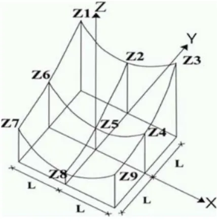
easily be generated once the basic parameters described in Eqs. (3) have been derived for cells according to the scheme in Fig. 3.
A=
hZ
1+Z3+Z7+Z9 4
−
Z
2+Z4+Z8+Z6 2
+Z5 i
L4
B =
h
Z1+Z3−Z7−Z9 4
−
Z2−Z8 2
+Z5 i
L3
C =
h
−Z1+Z3−Z7−Z9 4
−
Z4−Z6 2
+Z5 i
L3 (3)
D=
h −Z4+Z6
2
−Z5 i
L2 E=
h
Z2+Z8 2
−Z5 i
L2
F =
h−Z
1+Z3+Z7−Z9 2
i
4L2 G=
[−Z4+Z6] 2L
H =[Z2
+Z8]
2L I=Z5
The 3×3 pixels kernel was selected for the DEM pixel size, since we considered a distance of 120 m sufficient to repre-sent the factors under study.
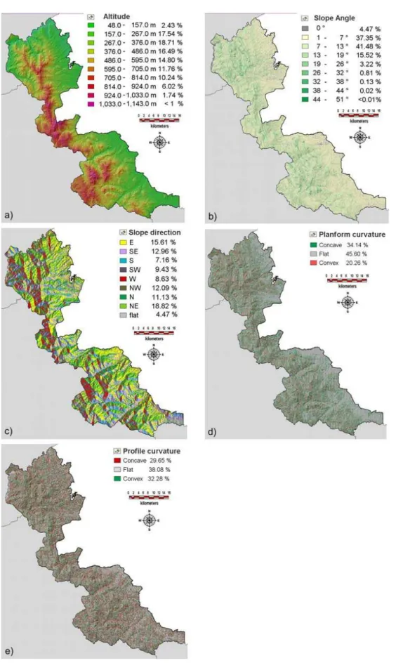
3.1.1 Altitude
The classification of the local reliefs needed in the statistical analysis was performed starting from the DEM, that contains elevation data related to each of the 40×40 m cells. Figure 4a shows the elevation dataset, also representing the prevailing morphology of the area. The whole territory is symbolized by around 3 billion points and altitudes ranging between 47 and 1143 m a.s.l.
3.1.2 Slope angle
Slope angle gradient is one the most important causes of slope instability (Ayalew and Yamagishi, 2005; Guzzetti et al., 1999; Kolat et al., 2006; Ohlmacher and Davis, 2003; Oyagi, 1984; S¨uzen and Doyuran, 2004; Zˆezere et al., 1999). The moisture content and pore pressure could be influenced at local scales, whereas the regional hydraulic behaviour could be controlled by slope angle patterns at larger scales. In accordance with the DEM post-spacing, the slope angle gradient is available over a regular 40×40 m grid. The slope
angle gradient is referred to cells and is calculated as the av-erage value (measured in sessagesimal degrees with respect to the proximal 8 cells) following the formula proposed by Zevenbergen and Thorne (1987)
Slope=arctan q
G2+H2
(4) In Fig. 4b a slope angle factor up to 51 degrees is shown.
Fig. 3.3×3 elevation sub-matrix used to assess morphometric fac-tors.
3.1.3 Slope exposure
Landslide distribution could potentially be affected by fac-tors related to the exposure of slopes with respect to the car-dinal directions. Slope exposure reveals possible influences of dominant winds, different weather conditions or effects related to the incident solar radiation. In particular, the latter effect on landslide occurrences has been suggested by Mossa et al. (2005) in the north-western part of the investigated area. As shown in Fig. 4c, slope exposure has been divided into 9 classes (E, SE, S, SW, W, NW, N, NE and flat areas). 3.1.4 Planform and profile curvatures
Curvatures analysis allows areas to be identified on a surface where convexities or concavities are more or less localized and, consequently, could help to identify zones that exhibit proneness to landsliding when such occurrences are related to these superficial features. Even if several algorithms for curvature analysis are available in GIS packages, the out-comes do not vary significantly when the elevation data are evenly spaced, as in the photogrammetric DEMs. For the sake of brevity and coherence with the causal factors dis-cussed above, only the results of the application of the Zeven-bergen and Thorne algorithm (1987) will be introduced. A concave (negative values) planform curvature could corre-spond to a convergence of the drainage lines and retaining of the water, whereas a planform curvature showing a con-vexity (positive values) could correspond to diverging flow lines (Lee and Min, 2001; Oh et al., 2009). Obviously, the local morphologies are more exhaustively drawn by the def-inition of a profile (longitudinal) curvature showing whether the slope is concave or convex. All these features are nor-mally related to some particular landslide kinematics or other slope instability phenomena, and influence the local drainage system.
3.2 Non-morphometric causal factors
Factors which are related to superficial features are grouped under the non-morphometric category even though at some stage of their computation a detailed knowledge of the mor-phology is required. Instead, the computation of some of the non-morphometric causal factors do not require any informa-tion on surface topography. This is the case of causal factors such as lithology and land cover, which are usually provided by means of vector maps at appropriate scales. In LR analy-sis their processing requires a rasterization procedure where attributes connected with geometric features have to be prop-erly managed in order to divide factors into separate classes. For instance, each pixel will be representative of a specific lithology or land cover class.
3.2.1 Drainage basin
Advanced tools available in GIS packages allow a new layer to be computed, with cell values expressing the cumulative flow that has passed through each cell during the drain pro-cess. The area drained by each pixel is, therefore, evaluated by means of a hierarchical dependency that is accomplished starting from the DEM. An average run-off rate is defined by the user and the same value is uniformly applied over the entire area. The algorithm assumes the run-off to be drained as overland flow and phenomena such as infiltration, perco-lation and evapotranspiration will not be taken into account in this layer. All these parameters could be implemented in the algorithm adopted, but a wide knowledge of these over the studied area is still far from complete at an eligible spa-tial accuracy. Results provided by the analysis are shown in Fig. 5a, where the draining capabilities are expressed as the numbers of cells drained by the reference pixel. Thanks to the introduction of this layer in the statistical analysis, a pos-sible relationship between the superficial run-off processes and the proneness to landslide is investigated. In addition, such an analysis is able to simulate the geographical run-off pattern under severe rainfall conditions, as well as showing the actual flows (Tarboton, 1997).
3.2.2 Lithology
Information on the lithology was derived from a series of 1:100 000 maps produced by the Servizio Geologico d’Italia (Italian Geological Agency) over the period from 1967 to 1975 (Cestari et al., 1975; Jacobacci et al., 1967; Jacobacci and Martelli, 1967; Malatesta et al., 1967). Maps were suc-cessively vectorized and lithologies assigned to geographical areas as attributes connected with vector polygons. In the statistical analysis, the original 36 classes of lithology were grouped into 11 new sub-classes on the basis of similarities in the lithological and geo-mechanical properties. The map reporting the lithology classes is shown in Fig. 5b.
3.2.3 Land cover
Land cover was derived from the classification of Land-sat 7 (sensor ETM+) Land-satellite data provided within the Corine Land Cover project (launched by the European Union Com-mission), after the validation by field survey. The spatial ac-curacy of these data could be related to a 1:50 000 map scale and, in order to reduce the number of variables involved in the analysis of this causal factor, the original classes of land cover were grouped into 9 classes on the basis of presumed similarities. Figure 5c reports the mapping of units in the Daunia Mts. area.
3.2.4 Distance from roads
A road segment may constitute a barrier or a corridor for wa-ter flow, a break in slope gradient or, in any case, may induce instability and slope failure mechanisms. The whole road network, composed of secondary roads was, therefore, in-cluded as a possible triggering factor and source of landslide susceptibility. The distance from the roads is computed as the minimum distance between each of the cells and the nearest road represented in vector format. This factor does not take into account the type of road (width, traffic intensity, rank, etc.). See Fig. 5d for a representation of this factor.
3.2.5 Distance from rivers
Previous studies carried out on a reduced portion of the Dau-nia Apennines by Mossa et al. (2005) highlighted a close spatial relation between the occurrence of landslides and the presence of watercourses or dense drainage lines. The “prox-imity to rivers” factor would potentially include an activating mechanism related to erosion along the slope foot. Unfortu-nately, ephemeral watercourses are not very easily express-ible in symbolic form in the vector data representing a river network, and it is very difficult to model the theory of wa-tercourses as triggers of landslide occurrences by data in a GIS. For this reason the causal factor discussed here must be interpreted as a search for a relationship between landslides and stable or permanent watercourses and rivers. As for the previous causal factor, the distances from rivers are evalu-ated by computing the minimum distance between cells and the nearest watercourse. See Fig. 5e for a representation of this factor.
3.3 Landslide inventory
1
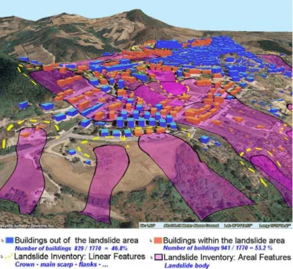
Fig. 6.Representation of the vector landslide inventory of an area enclosing the municipality of Bovino (FG). Buildings located within the mapped landslide are highlighted by means of a spatial query in GIS and coloured in red.
with attributes related to some of the fundamental parame-ters used in the description of the landslide body and possible landslide mechanisms. See Fig. 6 for a layout of the inven-tory with elevation data and aerial images superimposed.
Identification of the landslide locations and delimitations was carried out by fieldwork, supported by analysis of the aerial images and historical data. The geo-database collects information related to 249 landslide bodies, in the surround-ings of the 25 municipalities, as geometrical and alphanumer-ical features. The geometralphanumer-ical and positioning accuracy of polygons representing landslides was validated by overlay-ing them on a recently released numerical map (scale 1:5000) covering the Daunia Apennines.
4 Data analysis by Logistic Regression
In this application the management and processing of data related to individual factors were carried out in the GIS en-vironment (Geomedia Pro, Intergraph), while the statistical analysis by LR was performed using the SPSS (Statistical Package for Social Sciences) after exporting data to suitable exchange formats. In the first step, the 10 selected causal factors were classified in 68 classes that constitute the coded independent variables dataset. Coded variables were then exported to ASCII format and imported into the statistical package to proceed with the LR analysis and assess the β
regression coefficients.
The dependent variables were derived from the landslide inventory after rasterizing polygons and then coding the cells falling in the landslide areas. In the multiple LR analysis cells could inherit attributes providing information on the presence or absence of phenomena within the 40×40 m sub-area. After recombining the coefficients, as seen in Eq. (2), the proneness to landslide was finally computed throughout the Daunia Apennines and a susceptibility map produced. The overall dataset consisted of 799 906 cells with a subsam-ple of 15 895 (corresponding to 2543 ha) representing cells where the occurrence of landslides was proven by field sur-vey. However, in order to form a homogeneous cells dataset with the presence/absence of landslides, an equal number of cells free from slope failures phenomena was randomly extracted from the whole dataset and used in the “train-ing” phase of the LR analysis. Thus, coefficients are deter-mined by the maximum likelihood criterion on a sample of 31 790 cells.
5 Validation
Table 1. Confusion matrix with validation sample constituted by the 25% of the overall sample (0: absence of phenomenon; 1: pres-ence of phenomenon, cut-off value: 0.5).
PREDICTED Correctly classified
(%) 0 1
OBSERVED 0 3135 809 79.5 1 421 3523 89.3 Overall (%) 84.4
Table 2. Confusion matrix with validation sample constituted by the 50% of the overall sample (0: absence of phenomenon; 1: pres-ence of phenomenon, cut-off value: 0.5).
PREDICTED Correctly classified
(%) 0 1
OBSERVED 0 6300 1700 78.8 1 861 7116 89.2 Overall (%) 84.0
In particular, the susceptibility analysis by LR was per-formed twice, starting with 75% and 50% of the overall sam-ple. The validation procedure, based on comparison with the 25% and 50% quotas, not used, provided the confusion ma-trices reported in Tables 1 and 2. The Tables reveal a sub-stantial stability of the overall performance, in both tests up to 84%, as well as no change in the regression coefficients.
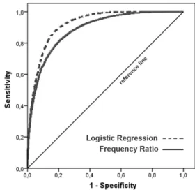
The ROC (Relative Operating Characteristic) is an alterna-tive approach to the assessment classification of the predic-tive rule. In the ROC analysis, the susceptibility map is com-pared with a dataset reporting the presence/absence of occur-rences in the same area. Values close to 1 indicate a very good fit (perfect classification) whereas a random fit of the model produces values of the Area Under the Curve (AUC) close to 0.5 in the ROC space. In this study, when starting with 75% of the overall sample a value of 0.923 was achieved in the AUC value (0.919 with 50% of the overall sample) and, consequently, the balance between the number of correctly classified pixels (true positives) and of incorrectly identified pixels (false positives) could be considered very satisfactory (see Fig. 7).
6 Results
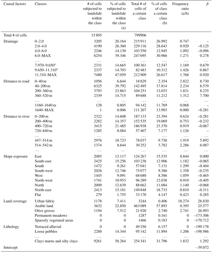
As discussed above, the relative importance of indepen-dent variables can be expressed by the regression coefficient, highlighting the causal factors and variables that are most strongly related to the occurrence of landslides (see Table 3 for a sub-set of the coefficients yielded by the LR analysis).
1
Fig. 7.ROC curves representing the prediction capability achieved by the Logistic Regression and Frequency Ratio analyses.
Land cover, lithology and exposure appear to be more strongly related to slope failure occurrences than other fac-tors. In particular, classes such as “permanent meadows” and “sparsely vegetated areas” show negative regression coeffi-cients and, therefore, act as protection against landslide oc-currences. On the other hand, a negative coefficient could be obtained if such classes are not present, or are assigned little weight in the training sample. Among the remaining classes, “urban and/or industrial fabric” and “arable land” exhibit positive, high regression coefficients and have to be considered as triggering factors.
Such a dependency could be related to the strong presence of urban fabric and arable land in the training areas, since the project was mainly focused on assessment of the landslide hazard in human settlement zones. Nevertheless, it should be stressed that, as pointed out by Akgun et al. (2008), both urbanized and cultivated areas result from heavier modifica-tions of the original landscape, and the instability phenomena could be triggered by such modifications. In addition, the two classes are inclined to be geographically linked because of their presence where the morphological pattern allows an-thropogenic alterations to be made. This trend is confirmed by the analysis of the “exposure” factor, which presents a positive coefficient only in sub-flat cells.
Coefficients related to the classes of lithology identify the “clays, marls and silty clays” as particularly prone to land-slide occurrences, while “terraced alluvial and fluvial de-posits” and “pebbles” exhibit negative coefficients.
Table 3.Results provided by the LR analysis. Coefficients are related to each of the classes created for single causal factors.
Causal factors Classes # of cells % of cells Total # of % of cells Frequency β
subjected to subjected to cells of of class ratio landslide landslide a certain a certain (a/b)
within within class class the class the class (b)
(a)
Total # of cells 15 895 799˙906
Drainage 0–2.0 3205 20.164 215 911 26.992 0.747 – 2.0–4.0 4190 26.360 229 116 28.643 0.920 –0.125 4.0–6.0 2246 14.130 103 550 12.945 1.092 –0.096 6.0–MAX 6254 39.346 247 695 30.966 1.271 0.278 . . . . 7.970–9.650◦ 2331 14.665 100 361 12.547 1.169 0.679
9.650–11.310◦ 2337 14.703 82 483 10.312 1.426 0.867 11.310–MAX 7480 47.059 212 909 26.617 1.768 0.920 Distance to road 0–40 m 1056 6.644 18 829 2.354 2.822 8.730 40–200 m 6325 39.792 142 495 17.814 2.234 8.579 200–360 m 3793 23.863 104 251 13.033 1.831 8.235 360–520 m 2339 14.715 89 688 11.212 1.312 7.700 . . . . 1160–1640 m 128 0.805 94 142 11.769 0.068 – 1640–MAX 1 0.006 111 207 13.903 0.000 –0.281 Distance to river 0–200 m 2322 14.608 187 133 23.394 0.624 –0.281 200–400 m 2282 14.357 152 535 19.069 0.753 –0.232 400–720 m 3415 21.485 186 938 23.370 0.919 –0.067 720–840 m 1285 8.084 57 407 7.177 1.126 – . . . . 447–514 m 2976 18.723 78 037 9.756 1.919 5.892 514–542 m 1374 8.644 30 252 3.782 2.286 6.087 . . . . Slope exposure East 2085 13.117 124 267 15.535 0.844 0.000 South-east 2425 15.256 103 238 12.906 1.182 –0.065 South 1472 9.261 57 041 7.131 1.299 –0.404 South-west 2026 12.746 75 077 9.386 1.358 –0.235 West 1445 9.091 68 680 8.586 1.059 –0.465 North-west 1741 10.953 96 289 12.038 0.910 –0.405 North 2009 12.639 88 662 11.084 1.140 –0.068 North-east 2413 15.181 149 848 18.733 0.810 –0.311 Flat 279 1.755 33 170 4.147 0.423 0.285 Land coverage Urban fabric 1178 7.411 3244 0.406 18.274 28.830 Arable land 3632 22.850 463 089 57.893 0.395 25.577 Olive groves 1194 7.512 21 920 2.740 2.741 26.993 Permanent meadows 0 0 1287 0.161 0 –173.306 Sparsely vegetated areas 0 0 1466 0.183 0 –170.712 Lithology Terraced alluvial 0 0 49 250 6.157 0 –199.178 Loose pebbles 2280 14.344 95 142 11.894 1.206 –198.986 . . . . Clays marns and silty clays 9261 58.264 254 341 31.796 1.832 1.292
1
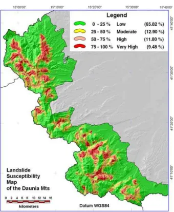
Fig. 8.Susceptibility map produced by the LR analysis.
The “distance from roads” factor is inversely proportional to the regression coefficients. This effect could be explained by the stress induced on a slope by a road, or a network of roads, in terms of the disruption of the natural profile, and the loads imposed by construction materials and vehicles. On the contrary, the “distance from rivers” factor is directly con-nected with the landslide susceptibility. Increasing distances (i.e. the absence of local stable drainage systems) correspond to higher positive regression coefficients. As reported by other authors, the absence of a drainage system could give rise to a higher level of soil saturation. In particular, a well-defined trend toward increasing coefficients is detected by the analysis for classes up to 720 m. Other causal factors do not show well-defined trends and their correlations with the oc-currence of landslides appear to be very weak. In addition to the regression coefficients, Table 3 includes the results pro-vided by the frequency ratio analysis that is very commonly performed beside the LR analysis. The ratio between the per-centage of cells subject to landslide within the class (a) and the overall percentage of cells in the same class (b) consti-tutes an “index of presence” assigned to such a class in areas threatened by slope instabilities, and helps to interpret the results provided by RL.
Finally, after recombining the coefficients with related classes of individual causal factors, a susceptibility map was produced. In Fig. 8, the susceptibility is expressed as prob-ability levels and a ranking of classes ranging from low to very high values is shown.
As shown in the map in Fig. 8, about 10% of the investi-gated area is classified as highly susceptible to landslides oc-currence, with probability levels ranging from 75% to 100%. This is not surprising since all the small municipalities in-volved in the study are continually threatened by slope fail-ure, and restoration of the transportation infrastructures is very often required after heavy rain phenomena.
7 Conclusions
The landslide susceptibility map prepared in the frame of the present work is a step forward in the management of land-slide hazard in the Daunia area. The LR methodology has demonstrated itself to be a suitable tool when the relation-ships between landslides and causal factors have to be anal-ysed. Such a result is achieved by the inspection of the re-gression coefficients that determine the role played by influ-encing factors on the investigated phenomenon. The “clays, marls and silty clays” class correspond to areas that are par-ticularly prone to landslide occurrences in addition to land coverage classes related to anthropogenic environments. As the main outcome of this work, a landslide susceptibility map was finally produced and validated. Up to 10% of the whole territory was assigned to the “high” susceptibility level, re-vealing also the geographical distribution of the areas most prone to landslide occurrences.
However, some weaknesses of this methodology have to be pointed out. Firstly, the analysis is still based on an input-output system due to the lack of full statistical capac-ity within the main GIS packages. In applying the LR model to the geographical data, an external package was necessary for the statistical analysis. However, these packages do not include advanced tools supporting the final mapping of re-sults produced by the analysis and so the resulting data have to be reintroduced into the GIS environment. Implementa-tion of the whole analysis in a single working GIS package is, therefore, essential to avoid time-consuming input-output procedures and other restrictions related to the use of sepa-rate applications. Secondly, owing to the low scale data used for such regional studies, the results are not very useful on a site-specific scale, where more detailed information and the geo-mechanical properties of landslides have to be consid-ered.
Acknowledgements. Research carried out within the project “Landslide risk assessment for the planning of small urban settlements within chain areas: the case of Daunia” (chief scientist: Federica Cotecchia, Technical University of Bari). Thanks are due to Francesca Santaloia (CNR-IRPI Bari) for the contribution to the GIS implementation of the landslide inventory with related geomorphological dataset. Software Geomedia Pro provided by Intergraph under the Synergy Programme.
Edited by: J. Huebl
Reviewed by: L. Saro and B. Pradhan
References
Akgun, A., Dag, S., and Bulut, F.: Landslide susceptibility mapping for a landslide-prone area (Findikli, NE of Turkey) by likelihood-frequency ratio and weighted linear combination models, Envi-ron. Geol., 54, 1127–1143, 2008.
Aleotti, P. and Chowdhury, R.: Landslide hazard assessment: sum-mary review and new perspectives, B. Eng. Geol. Environ., 58, 21–44, 1999.
Ayalew, L., Yamagishi, H., Marui, H., and Kanno, T.: Landslides in Sado Island of Japan: Part II. GIS-based susceptibility mapping with comparisons of results from two methods and verifications, Eng. Geol., 81, 432–445, 2005a.
Ayalew, L. and Yamagishi, H.: The application of GIS-based logis-tic regression for landslide susceptibility mapping in the Kakuda-Yahiko Mountains, Central Japan, Geomorphology, 65(1–2), 15– 31, 2005b.
Cestari, G., Malferrari, N., Manfredini, M., and Zattini, N.: Carta Geologica d’Italia 1:100 000 – Foglio 162, Servizio Geologico Italiano, 1975 (in Italian).
Chau, K. T. and Chan, J. E.: Regional bias of landslide data in generating susceptibility maps using logistic regression: Case of Hong Kong Island, Landslide, 2, 280–290, 2005.
Chen, Z. and Wang, J.: Landslide hazard mapping using logistic regression model in Mackenzie Valley, Canada, Nat. Hazards, 42(1), 75–89, 2007.
Cotecchia, F., Lollino, P., Santaloia, F., Vitone, C., and Mitaritonna, G.: A research project for deterministic landslide risk assessment in Southern Italy: methodological approach and preliminary re-sults, in: Proceedings of the 2nd International Symposium on Geotechnical safety and Risk IS-GIFU, Gifu, Japan, 11–12 June 2009.
Cotecchia, F., Santaloia, F., Lollino, P., Vitone, C., and Mitaritonna, G.: Deterministic landslide hazard assessment at regional scale, in: Proceedings of Geoflorida 2010, Advances in Analysis, Mod-eling and Design, West Palm Beach, Florida, US, 20–24 Febru-ary 2010.
Cotecchia, V.: I dissesti franosi del Subappennino Dauno con riguardi alle stradi provinciali, La Capitanata, 5–6, 1963. Dai, F. C. and Lee, C. F.: Landslide characteristics and slope
insta-bility modeling using GIS, Lantau Island, Hong Kong, Geomor-phology, 42(3–4), 213–228, 2002.
Dai, F. C., Lee, C. F., and Ngai, Y. Y.: Landslide risk assessment and management: an overview, Eng. Geol., 64(1), 65–87, 2002. Ercanoglu, M. and Gokceoglu, C.: Use of fuzzy relations to
pro-duce landslide susceptibility map of a landslide prone area (West Black Sea Region, Turkey), Eng. Geol., 75, 229–250, 2004.
Fayyad, U. and Irani, K.: Multi-interval discretization of continuous-value attributes for classification learning, Proceed-ings of the Thirteenth International Joint Conference on Artifi-cial Intelligence, San Mateo, CA, USA, 28 August–3 September 1993.
Guzzetti, F., Carrara, A., Cardinali, M., and Reichenbach, P.: Land-slide hazard evaluation: a review of current techniques and their application in a multi-scale study, Central Italy, Geomorphology, 31(1–4), 181–216, 1999.
Guzzetti, F., Reichenbach, P., Ardizzone, F., Cardinali, M., and Galli, M.: Estimating the quality of landslide susceptibility mo-dels, Geomorphology, 81(1–2), 166–184, 2006.
Hosmer, D. W. and Lemeshow, S. (Eds.): Applied logistic regres-sion, Wiley Interscience, New York, 2000.
Iovine, G., Parise, M., and Crescenzi, E.: Analisi della franosit`a nel settore centrale dell’Appennino Dauno, Mem. Soc. Geol. It., 51, 633–641, 1996.
Jacobacci, A. and Martelli, G.: Carta Geologica d’Italia 1:100 000 – Foglio 174, Servizio Geologico Italiano, 1967 (in Italian). Jacobacci, A., Malatesta, G., Martelli, G., and Stampanoni, G.:
Carta Geologica d’Italia 1:100 000 – Foglio 163, Servizio Ge-ologico Italiano, 1967 (in Italian).
Kolat, C¸ ., Doyuran, V., Ayday, C., and S¨uzen, M. L.: Preparation of a geotechnical microzonation model using Geographical Infor-mation Systems based on Multicriteria Decision Analysis, Eng. Geol., 87, 241–255, 2006.
Lee, S. and Min, K.: Statistical analysis of landslide susceptibility at Yongin, Korea, Environ. Geol., 40, 1095–1113, 2001. Lee, S. and Sambath, T.: Landslide susceptibility mapping in the
Damrei Romel area, Cambodia using frequency ratio and logistic regression models, Environ. Geol., 50(6), 847–855, 2006. Lee, S., Ryu, J. H., and Kim, I. S.: Landslide susceptibility analysis
and its verification using likelihood ratio, logistic regression and artificial neural network models: case study of Youngin, Korea, Landslides, 4, 327–338, 2007.
Lee, S. and Pradhan, B.: Landslide hazard mapping at Selangor, Malaysia using frequency ratio and logistic regression models, Landslides, 4, 33–41, 2007.
Malatesta, G., Perno, U., and Stampanoni, G.: Carta Geologica d’Italia 1:100 000 – Foglio 175, Servizio Geologico Italiano, 1967 (in Italian).
Menard, S.: Applied Logistic Regression, Second Edition, Sage University Paper on Quantitative Applications in the Social Sci-ences, 106, Thousands Oaks, California, US, 2001.
Mossa, S., Capolongo, D., Pennetta, L., and Wasowski, J.: A GIS-based assessment of landsliding in the Daunia Apennines, South-ern Italy, in: Proceedings of the conference “Mass movement hazard in various environments”, Polish Geological Institute spe-cial papers, 20, 86–91, 2005.
Nandi, A. and Shakoor, A.: A GIS-based landslide susceptibility evaluation using bivariate and multivariate statistical analyses, Eng. Geol., 110, 11–20, 2009.
O’Sullivan, D. and Unwin, D. J. (Eds.): Geographical Information Analysis, Wiley, New Jersey, USA, 2003.
Ohlmacher, G. C. and Davis, J. C.: Using multiple logistic regres-sion and GIS technology to predict landslide hazard in northeast Kansas, USA, Eng. Geol., 69, 331–343, 2003.
Oyagi, N.: Landslides in weathered rocks and residuals soils in Japan an surrounding areas: state-of-the-art report, in: Proceed-ings of the 4th International Symposium on Landslides, Toronto, 1–31, 16-21 September 1984.
Pradhan, B., Lee, S., and Buchroithner, M. F.: Use of geospatial data for the development of fuzzy algebraic operators to landslide hazard mapping: a case study in Malaysia, Applied Geomatics, 1, 3–15, 2009.
Pradhan, B. and Lee, S.: Landslide susceptibility assessment and factor effect analysis: backpropagation artificial neural networks and their comparison with frequency ratio and bivariate logistic regression modelling, Environ. Modell. Softw., 25(6), 747–759, 2010a.
Pradhan, B. and Lee, S.: Regional landslide susceptibility analysis using back-propagation neural network model at Cameron High-land, Malaysia, Landslides, 7(1), 13–30, 2010b.
Santacana, N., Baeza, B., Corominas, J., De Paz, A., and Mar-turi´a, J.: A GIS-Based Multivariate Statistical Analysis for Shal-low Landslide Susceptibility Mapping in La Pobla de Lillet Area (Eastern Pyrenees, Spain), Nat. Hazards, 30, 281–295, 2003. S¨uzen, M. L. and Doyuran, V.: Data driven bivariate landslide
sus-ceptibility assessment using geographical information systems: a method and application to Asarsuyu catchment, Turkey, Eng. Geol., 71, 303–321, 2004.
Tarboton, D. G.: A new method for the determination of flow di-rections and contributing areas in grid Digital Elevation Models, Water Resour. Res., 33(2), 309–319, 1997.
Vijith, H. and Madhu, G.: Estimating potential landslide sites of an upland sub-watershed in Western Ghat’s of Kerala (India) through frequency ratio and GIS, Environ. Geol., 55, 1397–1405, 2008.
Vitone, C., Cotecchia, F., Desrues, J., and Viggiani, G.: An ap-proach to the interpretation of the mechanical behaviour of in-tensely fissured clays, Soils Found., 49(3), 355–368, 2009. Yalcin, A.: GIS-based landslide susceptibility mapping using
an-alytical hierarchy process and bivariate statistics in Ardesen (Turkey): Comparisons of results and confirmations, Turkey, Catena, 72, 1–12, 2008.
Yesilnacara, E. and Topalb, T.: Landslide susceptibility mapping: A comparison of logistic regression and neural networks methods in a medium scale study, Hendek region (Turkey), Eng. Geol., 79, 251–266, 2005.
Zevenbergen, L. W. and Thorne, C. R.: Quantitative analysis of land surface topography, Earth Surf. Proc. Land., 12, 47–56, 1987. Zˆezere, J. L., de Brum Ferreira, A., and Rodrigues, M. L.: The
role of conditioning and triggering factors in the occurrence of landslides: a case study in the area north of Lisbon (Portugal), Geomorphology, 30, 133–146, 1999.