www.atmos-chem-phys.net/16/3683/2016/ doi:10.5194/acp-16-3683-2016
© Author(s) 2016. CC Attribution 3.0 License.
Validation of the Swiss methane emission inventory by atmospheric
observations and inverse modelling
Stephan Henne1, Dominik Brunner1, Brian Oney1, Markus Leuenberger2, Werner Eugster3, Ines Bamberger3,4, Frank Meinhardt5, Martin Steinbacher1, and Lukas Emmenegger1
1Empa Swiss Federal Laboratories for Materials Science and Technology, Überlandstrasse 129, Dübendorf, Switzerland 2Univ. of Bern, Physics Inst., Climate and Environmental Division, and Oeschger Centre for Climate Change Research, Bern, Switzerland
3ETH Zurich, Inst. of Agricultural Sciences, Zurich, Switzerland
4Institute of Meteorology and Climate Research Atmospheric Environmental Research (IMK-IFU), Karlsruhe Institute of Technology (KIT), Garmisch-Partenkirchen, Germany
5Umweltbundesamt (UBA), Kirchzarten, Germany
Correspondence to:Stephan Henne ([email protected])
Received: 30 October 2015 – Published in Atmos. Chem. Phys. Discuss.: 16 December 2015 Revised: 10 March 2016 – Accepted: 14 March 2016 – Published: 21 March 2016
Abstract. Atmospheric inverse modelling has the potential to provide observation-based estimates of greenhouse gas emissions at the country scale, thereby allowing for an inde-pendent validation of national emission inventories. Here, we present a regional-scale inverse modelling study to quantify the emissions of methane (CH4) from Switzerland, making use of the newly established CarboCount-CH measurement network and a high-resolution Lagrangian transport model. In our reference inversion, prior emissions were taken from the “bottom-up” Swiss Greenhouse Gas Inventory (SGHGI) as published by the Swiss Federal Office for the Environ-ment in 2014 for the year 2012. Overall we estimate national CH4emissions to be 196±18 Gg yr−1for the year 2013 (1σ uncertainty). This result is in close agreement with the re-cently revised SGHGI estimate of 206±33 Gg yr−1 as re-ported in 2015 for the year 2012. Results from sensitivity inversions using alternative prior emissions, uncertainty co-variance settings, large-scale background mole fractions, two different inverse algorithms (Bayesian and extended Kalman filter), and two different transport models confirm the ro-bustness and independent character of our estimate. Accord-ing to the latest SGHGI estimate the main CH4source cate-gories in Switzerland are agriculture (78 %), waste handling (15 %) and natural gas distribution and combustion (6 %). The spatial distribution and seasonal variability of our poste-rior emissions suggest an overestimation of agricultural CH4
1 Introduction
Atmospheric methane (CH4) acts as an important greenhouse gas (GHG) whose man-made increase from pre-industrial to present-day levels (from ≈700 nmol mol−1 in 1750 to 1819 nmol mol−1in 2012) directly and indirectly contributes 0.97 (0.74–1.20) W m−2to present-day global radiative forc-ing (Myhre et al., 2013). As such, its contribution to human-induced global warming is second only to carbon dioxide (CO2). Globally, natural sources (wetlands, lakes, geolog-ical seeps, termites, methane hydrates, and wild animals) and anthropogenic sources (fossil fuel extraction, distribu-tion and combusdistribu-tion, rice cultivadistribu-tion, ruminants, and waste) each contribute about half to CH4 emissions to the atmo-sphere (Kirschke et al., 2013), but larger uncertainties are connected with the natural sources. Owing to increased re-search efforts in recent years, uncertainties associated with these fluxes have decreased on the global and continental scale (Kirschke et al., 2013, and references therein). How-ever, there remain open questions about the contributing pro-cesses and their temporal and spatial distributions on the re-gional scale (Nisbet et al., 2014).
In many developed countries, natural CH4sources are of limited importance (Bergamaschi et al., 2010) and anthro-pogenic emissions dominate. For example,≈98 % of Swiss CH4 emissions are thought to be of anthropogenic origin (Hiller et al., 2014a). Owing to its comparatively short at-mospheric lifetime (≈10 years), CH4has been classified as a short-lived climate pollutant, and reducing anthropogenic CH4emissions has become a promising target to lower near-term radiative forcing (Ramanathan and Xu, 2010; Shindell et al., 2012). However, the development of efficient miti-gation strategies requires detailed knowledge of the source processes and the success of the mitigation measures should be monitored once put into action. The Kyoto Protocol sets legally binding GHG emission reduction targets for Annex I countries and the United Nations Framework Convention on Climate Change (UNFCCC) calls signatory countries to re-port their annual GHG emissions of CO2, CH4, nitrous oxide, sulfur hexafluoride, and halocarbons.
In Switzerland, the Federal Office for the Environment (FOEN) collects activity data and emission factors in the Swiss Greenhouse Gas Inventory (SGHGI) (FOEN, 2014, 2015) and annually reports emissions following IPCC guide-lines (IPCC, 2006). According to this inventory, emis-sions from agriculture are the single most important source (161.5 Gg yr−1) in Switzerland, followed by waste handling (32.3 Gg yr−1) and fossil fuel distribution and combustion (12.1 Gg yr−1; all values refer to the 2015 reporting for the year 2012). Estimates following IPCC guidelines are de-rived bottom-up from source-specific information combined with activity data and other statistical data, all of which may contain considerable uncertainties. Anthropogenic CH4 emissions in Switzerland originate from processes that may vary strongly on an individual basis (e.g. ruminants,
ma-nure handling, waste treatment). Hence, at the country level they are much more difficult to quantify than anthropogenic emissions of CO2, which can be largely deduced from fuel statistics. As a consequence, the uncertainty assigned to to-tal Swiss CH4 emissions (±16 %) is much larger than that of CO2emissions (±3 %) (FOEN, 2015). According to the SGHGI, Swiss CH4emissions have decreased by about 20 % since 1990 (FOEN, 2015), but given the above uncertain-ties, these estimates require further validation, also in order to survey the effectiveness of the realised reduction mea-sures. Furthermore, considerable differences exist between the SGHGI and other global- and European-scale invento-ries (e.g. EDGAR) both in terms of total amount and spatial distribution (Hiller et al., 2014a). Previous validation efforts of the Swiss CH4inventory were restricted to flux measure-ments either on the site scale focusing on a specific emission process (Eugster et al., 2011; Tuzson et al., 2010; Schroth et al., 2012; Schubert et al., 2012) or campaign-based flight missions (Hiller et al., 2014b) and tethered balloon sound-ings (Stieger et al., 2015), mainly confirming estimates of the SGHGI on the local scale. In addition, mobile near-surface measurements were used to verify emission hotspots in a qualitative way (Bamberger et al., 2014). However, due to the limited number of studies and the focus on rather small areas, it is very difficult to employ these results for the vali-dation of national total emission estimates.
pro-cesses: oil and gas extraction, ruminants, and natural gas dis-tribution to the end user.
Here, we validate the bottom-up estimate of Swiss CH4 emissions as given in the SGHGI by analysing continu-ous, near-surface observations of CH4 from the newly es-tablished, dense CarboCount-CH measurement network in central Switzerland (Oney et al., 2015) and two neighbour-ing sites. For the first time, we apply an inverse modellneighbour-ing framework with high spatial resolution (<10 km) to a rel-atively small area with considerable land surface hetero-geneity and topographical complexity. Such modelling ap-proaches have only recently become feasible through the use of high-resolution atmospheric transport simulations (e.g. for CH4; Zhao et al., 2009; Jeong et al., 2012, 2013; McKain et al., 2015). The main aim of the study is to provide an in-dependent validation of the SGHGI in terms of national total emissions (FOEN, 2015), geographical (Hiller et al., 2014a) and temporal distribution. Results in the spatio-temporal dis-tribution shall be used to draw conclusions on the estimates of individual source processes.
2 Data and methods 2.1 Observations
The CH4 observations used in this study are those of the CarboCount-CH1network (BEO, LHW, FRU, GIM) located on the Swiss Plateau and those from two additional moun-tain sites: Jungfraujoch and Schauinsland (see Figs. 1, S1 in the Supplement and Table 1). The Swiss Plateau, the rela-tively flat area between the Alps in the south and Jura Moun-tains in the north, covers only about one-third of the area of Switzerland but is home to two-thirds of the Swiss pop-ulation and is characterised by intensive agriculture and ex-tended urban and suburban areas. Approximately two-thirds of the Swiss CH4 emissions are thought to stem from this area (Hiller et al., 2014a). Oney et al. (2015) characterised the transport to the CarboCount-CH sites applying the same transport model as used here. They find that all four sites are mainly sensitive to emissions from most of the Swiss Plateau during summer daytime conditions, whereas sensitivities are more localised around the sites in winter but still provide rea-sonable coverage of the targeted area of the Swiss Plateau.
The Beromünster (BEO) site is located on a hill in an in-tensively used agricultural area. It is surrounded mainly by croplands and to a smaller extent rangeland. The site itself consists of a 217 m high decommissioned radio transmission tower. Gas inlets and meteorological instrumentation are in-stalled on the tower at five different heights above ground (12 to 212 m), whereas the gas analyser is located at the foot of the tower. A comprehensive description of the installa-tion and the measurement system can be found in Berhanu et al. (2015). Here, only the observations from the topmost
1http://www.carbocount.ch, last accessed 9 September 2015
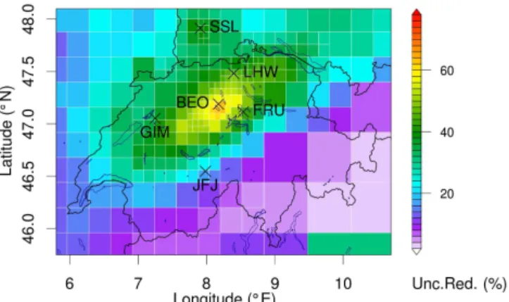
Figure 1.Total source sensitivity for the period March 2013 to February 2014 and the 4 sites used in the base inversion (crosses and labels in subplot – BEO: Beromünster; LHW: Lägern Hochwacht; JFJ: Jungfraujoch; SSL: Schauinsland). Source sensitivities are dis-played on the reduced resolution grid that is used in the inversion. The units of the source sensitivity are given as residence times di-vided by atmospheric density and surface area. The locations of the two validation sites (FRU: Früebüel; GIM: Gimmiz) are given in the subplot as well.
inlet height (212 m) were used, since this height showed the largest extent of the relative footprint and, hence, is least in-fluenced by local sources (Oney et al., 2015).
Lägern Hochwacht (LHW) is a mountaintop site on a very steep, west–east-extending crest approximately 15 km north-west of and 400 m above the city centre of Zurich, the largest city in Switzerland. The site is surrounded by forest with av-erage tree crown heights of 20 m close to the site. The gas in-let and meteorological instrumentation is mounted on a small tower of 32 m.
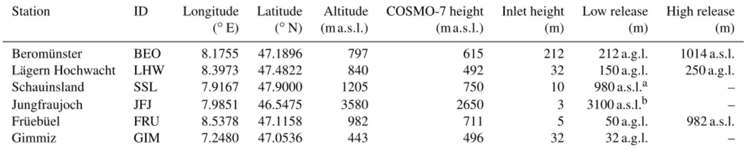
deter-Table 1.Overview of the location of the observational sites used in the study, including particle release heights as used in FLEXPART simulations. See text for details on release height selection.
Station ID Longitude Latitude Altitude COSMO-7 height Inlet height Low release High release
(◦E) (◦N) (m a.s.l.) (m a.s.l.) (m) (m) (m)
Beromünster BEO 8.1755 47.1896 797 615 212 212 a.g.l. 1014 a.s.l.
Lägern Hochwacht LHW 8.3973 47.4822 840 492 32 150 a.g.l. 250 a.g.l.
Schauinsland SSL 7.9167 47.9000 1205 750 10 980 a.s.l.a –
Jungfraujoch JFJ 7.9851 46.5475 3580 2650 3 3100 a.s.l.b –
Früebüel FRU 8.5378 47.1158 982 711 5 50 a.g.l. 982 a.s.l.
Gimmiz GIM 7.2480 47.0536 443 496 32 32 a.g.l. –
a920 m a.s.l. in FLEXPART-ECMWF.b3000 m a.s.l. in FLEXPART-ECMWF.
mined by comparing differences between the observations of BEO (212 m), which exhibit less local influences, and FRU as a function of wind speed and direction at FRU.
At the Gimmiz site (GIM, 443 m a.s.l.) sample gases are drawn from a 32 m tall water tower. The surrounding area is flat and dominated by intensive agriculture, mostly veg-etable farming and croplands. The area is a transformed wet-land that used to be regularly flooded until the 1850s before the levelling of the river system (1868–1891), when former wetlands were also converted to agricultural lands (Schnei-der and Eugster, 2007). Although there are only two small farms in the direct vicinity, larger potential CH4sources are located in the town of Aarberg about 2.5 km to the south-east. Here a sugar refinery, operating a large-scale waste wa-ter treatment plant (250 000-person equivalent), a compost and soil recycling facility, and a biogas reactor for electrical power generation are located. These local sources may not be represented sufficiently well in model simulations. There-fore and as in the case of FRU, observations from GIM were filtered by wind speed and direction, excluding all 10 min av-erages for which wind speeds were either below 2 m s−1or coming from directions between 90 and 150◦. Again, these thresholds were estimated by comparison to the observations at BEO.
Schauinsland (SSL, 1205 m a.s.l.) is a mountaintop site in the Black Forest, Germany, to the north of the Swiss Plateau. As such it is usually situated above the stable nocturnal boundary layer of the surrounding, but at daytime it is af-fected by boundary layer air (Schmidt et al., 1996). The site is surrounded by forests and rangeland and no large CH4source is known in the direct vicinity. While not part of CarboCount-CH network, the observations from SSL provide additional constraints for the atmospheric inversion, especially at mid-distance from the Swiss Plateau.
The high-altitude observatory Jungfraujoch (JFJ, 3580 m a.s.l.) is located in the northern Swiss Alps on a steep mountain saddle between the two mountains Jungfrau (4158 m a.s.l.) and Mönch (4099 m a.s.l.). Al-though JFJ is usually located in the free troposphere, it intermittently receives polluted boundary layer air from
sources both north and south of the Alps (Zellweger et al., 2003; Henne et al., 2010; Tuzson et al., 2011). The intensity of these transport events from the boundary layer can vary strongly depending on the weather condition and the transport process responsible for lifting.
At all sites, CH4 measurements were carried out us-ing PICARRO (Santa Clara, CA, USA) cavity rus-ing-down spectrometers (Rella et al., 2012), which provide high-frequency (approximately 0.5 to 1 Hz) observations of CO2, CH4, H2O and (at BEO and LHW) CO. All instruments were calibrated against the WMO X2004 CH4 scale (Dlu-gokencky et al., 2005) and were reporting dry air mole fractions by either applying a water vapour correction ac-counting for dilution and spectroscopic effects (CarboCount-CH sites and SSL) or by using pre-sample drying of sam-ple air (JFJ). At the CarboCount-CH sites, measurements of additional target gases, not used for the calibration, give an estimate of the instruments’ non-random uncer-tainty for CH4 of ≈0.5 nmol mol−1 (Oney et al., 2015). At SSL observations of three additional target gases yield a combined measurement uncertainty of 0.3 nmol mol−1. For JFJ a combined measurement uncertainty of σ= q
0.312+ 3.61×10⁻⁴×χ2nmol mol−1 was reported for hourly aggregates, where χ is the observed mole fraction (Empa, 2015).
the sites are least influenced by small-scale, thermally in-duced flow systems in the complex topography around the sites. Since the sites are situated on mountaintops no devel-opment of a shallow night-time boundary layer is expected so that the influence of local sources (if at all present) re-mains negligible at night. All of the following analysis and discussion is based on this filtered and aggregated data set. In addition to the absolute mole fraction, an estimate of larger-scale background mole fractions, which represent conditions without recent emission input, was generated using the “ro-bust estimation of baseline signal” (REBS) method (Ruck-stuhl et al., 2012). We refer to this term as baseline mole fraction in the following. It represents a smooth curve fitted to the data, providing a baseline mole fraction for each obser-vational time. The absolute mole fraction of the observations, χo, can then be given as the sum of the baseline,χo,b, and the contribution due to recent emissions,χo,p,
χo=χo,p+χo,b. (1)
The REBS method iteratively fits a non-parametric lo-cal regression curve to the observations, successively ex-cluding points outside a certain range around the baseline curve. REBS was applied separately to hourly data from each site using asymmetric robustness weights with a tun-ing factor of b=3.5, a temporal window width of 60 days and a maximum of 10 iterations. An estimate of the base-line uncertainty is given by REBS as a constant value for the whole time series. For JFJ the baseline uncertainty was estimated to 17.4 nmol mol−1, whereas uncertainties for the other sites ranged between 16.2 nmol mol−1 (SSL) and 18.9 nmol mol−1(LHW). The larger values generally reflect a larger degree of variability in the baseline and a reduced frequency of air masses not influenced by recent surface con-tact and emissions.
2.2 Transport models
Source sensitivities giving the direct influence of a mass emission from a source location onto the mole fraction at a receptor site were calculated with two different versions of the Lagrangian particle dispersion model (LPDM) FLEX-PART (Stohl et al., 2005), which can be run in time-inverted mode. The first represents the standard FLEXPART model (version 9.02) driven by analysis fields of the operational runs of the Integrated Forecast System (IFS) of the European Centre for Medium Range Weather Forecast (ECMWF). In-put fields were available every 3 h with a horizontal resolu-tion of 0.2◦×0.2◦(≈15 km× ≈22 km) for the Alpine area (−4 to 16◦E and 39 to 51◦N) and 1◦×1◦elsewhere. The second FLEXPART version is the one adapted to the use of output from the COSMO regional numerical weather pre-diction (NWP) model (Baldauf et al., 2011). FLEXPART-COSMO was driven by operational analysis fields as gen-erated hourly by the Swiss national weather service, Me-teoSwiss, for western Europe (approximately −10 to 20◦E
and 38 to 55◦N) with a horizontal resolution of approxi-mately 7 km×7 km. Hourly analysis fields are produced ap-plying an observational nudging technique (Schraff, 1997) to near-surface and vertical profile observations of pressure, rel-ative humidity and wind. The use of a high-resolution trans-port model in regional-scale inversions based on point ob-servations is a prerequisite to reduce the representation un-certainty of the model (Tolk et al., 2008; Pillai et al., 2011). Furthermore, the use of a time-inverted LPDM is highly ben-eficial to this purpose as it allows an accurate transport de-scription in the near-field of the sites below the resolution of the driving meteorology.
The main differences between FLEXPART-COSMO and standard FLEXPART-ECMWF are the internal vertical grid representation and the parameterisation of convective trans-port. In FLEXPART-COSMO, the native vertical grid of the COSMO model is used as the main frame of reference, which, in this case, was a height-based hybrid coordinate sys-tem (Gal-Chen and Somerville, 1975). In contrast, standard FLEXPART uses a terrain-following vertical coordinate with constant level depths up to the model top, which requires an initial vertical interpolation from the pressure-based hybrid coordinate used in the IFS. In FLEXPART-COSMO, all in-terpolation to particle positions is done directly from the na-tive COSMO grid, avoiding multiple interpolation errors. In FLEXPART-ECMWF sub-grid-scale convection is treated by an Emanuel-type scheme (Emanuel and Zivkovic-Rothman, 1999; Forster et al., 2007), whereas in FLEXPART-COSMO the same modified version of the Tiedtke convection scheme (Tiedtke, 1989) as used in COSMO was implemented.
PBL heights are a critical parameter in FLEXPART since they are used as a scaling parameter for the turbu-lence parameterisation. We use the default implementation within FLEXPART to diagnose PBL heights applying a bulk Richardson method (Stohl et al., 2005; Vogelezang and Holt-slag, 1996). In contrast to standard FLEXPART we did not use 2 m temperatures from COSMO in the PBL estimation but the lowest model level temperature (approximately 10 m above ground), because FLEXPART and COSMO PBL heights showed a positive bias when compared to PBL height observations from the sounding site Payerne on the Swiss Plateau under convective conditions and when using 2 m temperatures (Collaud Coen et al., 2014). This bias disap-peared when using the first level temperatures instead.
Therefore, we chose to release particles at two vertical loca-tions for the CarboCount-CH sites to analyse the sensitivity of this choice. At BEO, where the model topography is rela-tively close to the site’s altitude, these span the possible range of reasonable release altitudes by representing (1) the height above model surface as given by the inlet height of the ob-servations and (2) the absolute altitude above sea level of the inlet. At the sites FRU and LHW the lower and higher release heights were chosen 50 m and 150 m above model ground, respectively, because height deficiencies in the model were larger there. At GIM only one release height was used be-cause the model topography was relatively close to the true surface altitude. Also, for the more remote sites JFJ and SSL, only one release height was simulated that represents the middle between the model surface and the site altitude. Previously it was shown that such an approach works best (independent of time of day) for the mountaintop site JFJ, which shows large model topography deficits (Brunner et al., 2013). Values for all release heights are given in Table 1. Note that release heights were the same for all FLEXPART-ECMWF and FLEXPART-COSMO simulations except for JFJ and SSL were surface height differences between the models were large.
From both models, output was generated on a regu-lar longitude–latitude grid with a horizontal resolution of 0.16◦×0.12◦ (≈13 km) covering western Europe and for a nested Alpine domain with a horizontal resolution of 0.02◦×0.015◦(≈1.7 km). The generated output represents the summed residence time, τi,j, of particles in a given grid box,i, j, and below a specific sampling height,hs, di-vided by the density of dry air in this grid cell and has units s m3kg−1gridcell−1. The sampling height was set to 50 and 100 m above ground in FLEXPART-COSMO and FLEXPART-ECMWF, respectively, coinciding with the min-imal PBL height used in the models. Multiplication ofτi,j with the volume of the sampling grid cell, Vi,j=Ai,j·hs, and the ratio of the molar weight of the species of interest, µs, and the molar weight of dry air, µd, yields the desired source sensitivity,mi,j, in units of s kg−1mol mol−1,
mi,j = τi,j
Vi,j µd µs
. (2)
Whenmi,j is multiplied by a mass emission in the same grid box,Ei,j (kg s−1), the product gives the effect this emission would have on the dry air mole fraction at the receptor. The sum over all grid boxes then yields the increase in mole frac-tion,χp, due to recent emissions, whereas the baseline mole fraction, χb, can be obtained as the average mole fraction over all particles at their end points in the simulation
χ=X
i,j
mi,jEi,j
| {z } χp
+ 1 K
K X
k χk
| {z } χb
, (3)
wherei, jare the horizontal grid indices,χkthe mole fraction at each particle’s end point, andKis the number of particles. In our FLEXPART-COSMO simulations particles were fol-lowed for 4 days backward in time. Not all particles leave the limited-area model domain during this time, so that the base-line mole fraction as given in Eq. (3) cannot be directly trans-lated to conditions at the domain boundaries, but may also contain contributions from within the domain and, therefore, may vary between different sites. For the inversion set-up it would be beneficial if the baseline mole fractions could be estimated from an external three-dimensional model. How-ever, such model input was not available at the time of anal-ysis, and thus the prior baseline mole fraction was taken as the one estimated from the observations (REBS) and further optimised in the inversion.
2.3 Inversion framework
In our inversion system the source sensitivities calculated by the transport model can be used to give a direct relationship between the simulated mole fractions and the so-called state vector,x=(x1. . . xK)with a total ofK elements, that pri-marily contains the desired gridded emissions. In matrix no-tation this can be expressed as
χ=Mx, (4)
where χ=(χ1. . . χL) represents the simulated mole frac-tions at different times and locafrac-tions,l=1, . . ., L. The sen-sitivity matrixM(dimensioned K×L) contains the sensi-tivities for each time/location towards thekth element of the state vector.
τB=5 days over the observation period and were optimised separately for each site, resulting in 73 baseline elements in the state vector for each site. Prior estimates of the base-line mole fractions were REBS estimates for the site JFJ (see Sect. 2.1). Since the REBS estimate represents a smooth curve to the data, the REBS value at the time of a given base-line node was used as its prior value.
In our base set-up we target temporal average emission fluxes for the period of observations (March 2013 to Febru-ary 2014) and optimise their spatial distribution. We include seasonality in the emission fluxes as part of our sensitivity analysis (see Sect. 2.5.2).
In order to reduce the size of the inversion problem, emis-sions were not optimised on a regular longitude–latitude grid as given by the FLEXPART simulations. Instead, a reduced grid was used that assigns finer (coarser) grid cells in ar-eas with larger (smaller) average source sensitivities. Start-ing from the finest output grid resolution of 0.02◦×0.015◦, four neighbouring grid cells were merged if their average residence time did not reach a specified threshold. This procedure was iterated up to a maximum grid cell size of 2.56◦×1.92◦. The residence time threshold was set manu-ally in order to reduce the number of cells in the inversion to the order of KE≈1000. The overall extent of the emis-sion grid was determined by (1) the extent of the COSMO-7 domain, (2) the existence of considerable CH4emissions (cut-off over the oceans) and (3) a minimum source sensi-tivity. Tests with larger and smaller inversion domains did not indicate significant influences on the deduction of Swiss emissions.
In Bayesian atmospheric inversion, prior knowledge of the state vector, xb, and its probability distribution is used to guide the optimisation process. Mathematically this can be expressed by formulating a cost functionJthat penalises de-viations from the prior state and differences between simu-lated and observed mole fractions (e.g. Tarantola, 2005)
J =1
2(x−xb) TB−1(
x−xb)
+1
2 Mx−χo T
R−1 Mx−χo, (5)
wherexdescribes the optimised andxbthe prior state vec-tor, and Mx−χo is the difference between simulated and
observed mole fractions. BandR give the uncertainty co-variance matrices of the prior state and the combined model– observation uncertainty. In Sect. 2.4 the structure of these matrices is discussed in more detail. Minimisation ofJyields the posterior state
x=xb+BMT
MBMT +R −1
χo−Mxb. (6)
In our implementation the inverse of S= MBMT−R, aL×Lmatrix, was calculated using LU factorisation (func-tion DGESVX in LAPACK). In addi(func-tion to the posterior
state, its uncertainty expressed as an uncertainty covariance matrix,A, can also be given (e.g. Tarantola, 2005):
A=B−BMTS−1MB. (7)
The total emissions and their uncertainty from a certain region or country can then be calculated as
E=
KE X
k
xkgk;σE2=gTAEg, (8)
where the vectorggives the fractional contribution of a
re-gion to an inversion grid cell andAEis the part ofAthat con-tains the uncertainty covariance of the posterior emissions. gk takes a value of 1 for a grid cell that is completely within the region and 0 for grid cells outside the region. For coarse inversion grid cells containing more than one region,gkwas calculated from higher-resolution population data, weighting per region contributions by population and not by land sur-face area. In the case of the present CH4inversion and the na-tional estimates for Switzerland this treatment was of minor importance but is more crucial for other species that exhibit sharp emission gradients more closely following the popula-tion distribupopula-tion (e.g. halocarbons).
In our base inversion, we used the Swiss MAIOLICA in-ventory (Hiller et al., 2014a), which is based on the total Swiss emissions estimated by FOEN (SGHGI) for the year 2011 and reported to UNFCCC in 2013. For areas outside Switzerland, prior emissions were taken from the European-scale inventory developed by TNO for the MACC-2 project (Kuenen et al., 2014) (TNO/MACC-2 hereafter) applying the same country-by-country scaling to 2011 values reported to UNFCCC in 2013.
2.4 Covariance design
This section details the construction of the uncertainty co-variance matricesBandRas used in the base inversion. Pa-rameters used to build the matrices were chosen based on experience and previous publications (see below). The sensi-tivity to these choices was investigated in a set of sensisensi-tivity inversions as described in Sect. 2.5.
Both uncertainty covariance matrices are symmetric block matrices. In the case ofB, one block,BE, describes the uncer-tainty covariances of the emission vector and a second block, BB, the uncertainty covariances of the baseline mole frac-tions. Within each block the off-diagonal elements were al-lowed to be non-zero. The diagonal elements ofBEwere set proportional (factorfE) to the prior emissions in the respec-tive grid cellBj,jE = fExb,j
2
assumed for the off-diagonal elements that decays exponen-tially with the distance between two grid cells (e.g. Röden-beck et al., 2003; Gerbig et al., 2006; Thompson and Stohl, 2014):
Bi,jE =e−di,jL q
Bi,iE q
Bj,jE , (9)
wheredi,jis the distance between two grid cell centres andL the correlation length. In this set-up the total squared uncer-tainty of the prior emissionsσE2=1TBE1, where1is a vec-tor of all ones, only depends on the settings of L andfE. For the base inversion L was fixed to 50 km and fE was adjusted to yield fixed relative uncertainties of the national estimate for Switzerland of 16 %, which is the uncertainty given for the Swiss bottom-up estimate (FOEN, 2015). The choice of 50 km was driven by the need for sufficient con-straints for neighbouring grid cells, whereas Hiller et al. (2014a) suggested a shorter length scale around 10 km based on a comparison of the spatial structures of the MAIOLICA, TNO/MACC-2 and EDGAR CH4inventories.
All diagonal elements ofBBwere set to a constant value, Bi,iB =fbσb2, whereσb is an estimate of any given baseline uncertainty andfbis a scaling factor. The off-diagonal ele-ments were set assuming an exponentially decaying correla-tion of the baseline uncertainty between baseline nodes at a given site
Bi,jB =e− Ti,j
τb q
Bi,iB q
Bj,jB , (10)
where Ti,j is the time difference between two nodes and τbis the temporal correlation length. In the base inversion, σb was obtained from the REBS fit of the JFJ observations (17.4 nmol mol−1),f
bwas set to unity, andτbto 14 days. As forL, the choice ofτbis somewhat arbitrary but governed by the need for sufficient constraints on the posterior solution without restricting adjustments too strongly.
In the case of temporally variable emissions (see Sect. 2.5.2), the state vectorx, the sensitivity matrix and the prior uncertainty matrix have to be extended.BEnow should treat spatial and temporal covariance of the state vector. In-dividual diagonal elements ofBE,Bi,iE, now refer to different emission locations and time, with the indexi running over both of these dimensions. The off-diagonal elements can then be given by
Bi,jE =e− Ti,j
τt e−di,jL q
Bi,iE q
Bj,jE , (11)
where, in addition to Eq. (9),Ti,j gives the time difference between two emission sets andτtis the temporal correlation length scale of the prior emissions.
The block matrixRcontains one block for each site used in the inversion. In its diagonal elements both the observa-tion and the model uncertainty were considered by quadratic
addition:
Ri,i=σo2+σmin2 +σsrr2χp2,i, (12)
whereσois the observation uncertainty as estimated for each 3-hourly CH4 average (see Sect. 2.1) and the second and third term are contributions of the model uncertainty. σmin represents a constant contribution, while the third term rep-resents an uncertainty contribution relative to the prior simu-lation of above-baseline concentrations,χp,i (Brunner et al., 2012). For the base inversion,σminandσsrr were estimated separately for each site from the model residuals (difference between simulated and observed mole fraction) of the prior simulation,χp,i, by fitting a straight line through root mean square errors (RMSEs) calculated for separate bins along χp,o. The choice of this method was motivated by the obser-vation that prior model residuals tend to increase with prior mole fractions. Estimating the model uncertainty from the prior model residuals has been suggested before by Stohl et al. (2009), whereσminwas estimated as the RMSE from the prior simulation, whereasσsrr was set to 0. In an addi-tional step this constant value was then forced to yield a nor-mal distribution of the nornor-malised model residuals. Further-more, Stohl et al. (2009) applied their uncertainty estimation in an iterative way using the model residuals from successive inversion runs. In our experience this may lead to underes-timated model uncertainties and we did not iterate our pro-cedure. These methods have in common that the results of the prior simulation influence the estimation ofR, therefore somewhat violating the independence of prior and model– observation uncertainties assumed in the Bayesian approach. Finally, off-diagonal elements of the model–observation un-certainty covariance matrix were assumed to follow an expo-nentially decaying correlation structure.
Ri,j =e− Ti,j
τo pRi,ipRj,j, (13)
whereTi,j is the time difference between two measurements andτo is the temporal correlation length that describes the autocorrelation in the model–observation uncertainty. In the base inversionτowas set to 0.5 days, a value previously used by other authors (e.g. Thompson et al., 2011) and associated with the inability of atmospheric transport models to cor-rectly simulate the diurnal cycle in the PBL. The uncertainty covariances between observations from different sites were set to 0.
2.5 Sensitivity inversions
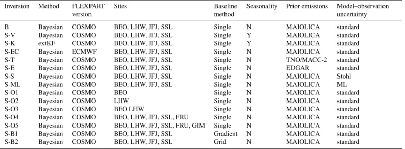
Table 2.Set-up of the base (B) and sensitivity inversions (S-X).
Inversion Method FLEXPART Sites Baseline Seasonality Prior emissions Model–observation
version method uncertainty
B Bayesian COSMO BEO, LHW, JFJ, SSL Single N MAIOLICA standard
S-V Bayesian COSMO BEO, LHW, JFJ, SSL Single Y MAIOLICA standard
S-K extKF COSMO BEO, LHW, JFJ, SSL Single Y MAIOLICA standard
S-EC Bayesian ECMWF BEO, LHW, JFJ, SSL Single N MAIOLICA standard
S-T Bayesian COSMO BEO, LHW, JFJ, SSL Single N TNO/MACC-2 standard
S-E Bayesian COSMO BEO, LHW, JFJ, SSL Single N EDGAR standard
S-S Bayesian COSMO BEO, LHW, JFJ, SSL Single N MAIOLICA Stohl
S-ML Bayesian COSMO BEO, LHW, JFJ, SSL Single N MAIOLICA ML
S-O1 Bayesian COSMO BEO Single N MAIOLICA standard
S-O2 Bayesian COSMO LHW Single N MAIOLICA standard
S-O3 Bayesian COSMO BEO LHW Single N MAIOLICA standard
S-O4 Bayesian COSMO BEO, LHW, JFJ, SSL, FRU Single N MAIOLICA standard S-O5 Bayesian COSMO BEO, LHW, JFJ, SSL, FRU, GIM Single N MAIOLICA standard S-B1 Bayesian COSMO BEO, LHW, JFJ, SSL Gradient N MAIOLICA standard
S-B2 Bayesian COSMO BEO, LHW, JFJ, SSL Grid N MAIOLICA standard
meet exactly in practice. In particular, potential systematic uncertainties in model transport, which may contribute im-portantly to the overall uncertainty (e.g. Gerbig et al., 2008), are not accounted for. To explore the range of uncertainty beyond the analytically derived posterior uncertainty and to test the robustness of the results to different assumptions, it has therefore been proposed to perform additional sensitivity inversions (e.g. Bergamaschi et al., 2010, 2015). To this end, we set up a series of sensitivity inversions that vary different aspects of the inversion (transport simulations, inversion al-gorithm, uncertainty covariance design, prior emissions, ob-servation selection, seasonality of emissions). An overview of these sensitivity inversions is given in Table 2 and details are described in the following.
2.5.1 Transport simulation
One important source of uncertainty when using observa-tional data from elevated sites is the potential mismatch be-tween model and real topography. The choice of the parti-cle release height in the model can considerably change the model’s performance and may lead to systematic biases in simulated concentrations. Therefore, we quantified the effect of the release height by using a “low” and “high” release case for each of the sensitivity inversions in Table 2. One is al-ways using the lower release heights for the CarboCount-CH stations as introduced in Sect. 2.2, whereas the other uses the higher release heights. The release heights of the more remote sites JFJ and SSL were not varied because of their less direct influence on the Swiss emissions. In addition to the release height, two different versions of the atmospheric transport model were used. The base inversion was based on FLEXPART-COSMO and a sensitivity run used the results of FLEXPART-ECMWF (S-EC).
2.5.2 Seasonal variability
In the base inversion emissions were assumed to be constant in time. However, considerable seasonal variability of the emissions especially from the agricultural sector can be ex-pected. To test the implication of this assumption, a sensitiv-ity run extending the state vector to separately hold emissions for each season (S-V) was set up following the common defi-nition of winter spanning the months December, January and February (DJF) and so forth (spring: MAM; summer: JJA; autumn: SON). The prior emissions and their uncertainty were set identical for all seasons. The correlation length scale between different emission times was set toτt =90 days (see Eq. 11). Reducing this time constant to 45 days had only a minor influence on the inverse emission estimate.
2.5.3 Inversion algorithm
uncer-tainty through the respective unceruncer-tainty covariance matri-cesBandR. In addition to these, the extKF requires an un-certainty covariance matrixQthat describes the uncertainty with which the state vector can change from one time step to the next.
Accordingly, uncertainties of the state vector are allowed to grow from one time step to the next, which introduces an additional amount of prior uncertainty as compared to the Bayesian approach. The matricesBandRwere parame-terised according to Eqs. (9) and (12), respectively. The cho-sen parameter values are listed in Table 3. The forecast uncer-tainty matrixQwas also parameterised according to Eq. (9), notably with the same spatial correlation length. The diago-nal elements ofQwere set to a relative forecast uncertainty of the emissions of 0.6 % per 24 h, which resulted in fairly constant posterior emissions in time with only a small sea-sonal cycle.
2.5.4 Covariance parameters
The next set of sensitivity inversions was designed to anal-yse the effect of different uncertainty covariance matrices. Our base inversion is based on the prior emission uncertainty as estimated by the SGHGI, which we consider to be the best knowledge of bottom-up uncertainty in Switzerland. Since Hiller et al. (2014a) used the same by-category emissions as the SGHGI to spatially disaggregate total emissions for the MAIOLICA inventory (our prior), we extrapolated the SGHGI uncertainty information to the whole inversion do-main. Next to the base inversion a set of uncertainty covari-ance parameters as estimated by the method of maximum likelihood (ML; Michalak et al., 2005) were used (S-ML). We estimated the covariance parameters (L,fE,τb, and indi-vidually for each sitefb,σmin,σsrr) by minimising the neg-ative logarithm of the likelihood estimator (Michalak et al., 2005)
Lθ= 1 2ln
MBMT +R
+1
2 χo−Mxb T
MBMT +R −1
χo−Mxb. (14)
As a consequence of the ML optimisation, posterior model residuals and posterior emission differences should follow a χ2 distribution. To find the minimum ofLθ a multivari-ate optimisation routine was used. We applied the Broyden– Fletcher–Goldfarb–Shanno (BFGS) algorithm that is widely used for optimisation problems (see, for example, Nocedal and Wright, 2006). Initial parameter values were set equal to those used in the base inversion, but giving all sites the same σminof 20 nmol mol−1andσsrrof 1. To assess the robustness of the ML optimisation results, an alternative algorithm was tested (Nelder–Mead), yielding very similar parameter sets.
Another sensitivity run varied the design of the model– observation uncertainty covariance by estimating the diago-nal elements of the matrix from the prior RMSE at each site
σmin=RMSE(χb−χo) and applying a correction for ex-treme residual values according to Stohl et al. (2009) (S-S). Such extreme residuals only occurred for two observations at LHW, so that essentially a constant model uncertainty was used for each site. The off-diagonal elements were calculated in the same way as in the base inversion. For the extKF inver-sion it was only possible to use a fixed set of parametersσmin andσsrr for all sites, because by-site treatment was not yet implemented in the current version of the code. They were selected to be close to the average values used in the refer-ence inversion. All covariance parameters used in the base, the ML approach, the Stohl et al. (2009) approach, and the extKF inversion are compared in Table 3. In the case of the Bayesian inversions, the covariance parameters differed be-tween the two release heights, with the high release showing larger values ofσminfor the sites BEO and LHW and all ap-plied estimation techniques.
2.5.5 Prior emissions
The sensitivity of the inversion result to the prior emissions was tested by using different prior inventories. In a sen-sitivity inversion we replaced the MAIOLICA emissions within Switzerland with those given by TNO/MACC-2 (S-T). A third sensitivity run was set up using the EDGAR (v4.2 FT2000) inventory for the base year 2010 (JRC/PBL, 2009) (S-E). In all three cases the prior uncertainty was set so that a value ofσE=16 % was reached for the Swiss emis-sions, which is the uncertainty given for the SGHGI (FOEN, 2015). For individual grid cells the resulting proportionality factor was fE≈30 %. However, the off-diagonal elements inBE contributed considerably to the total country uncer-tainty since they were especially large for small grid cells (see Fig. S2 in the Supplement).
2.5.6 Selection of observations
Another series of sensitivity inversions was set up using dif-ferent parts of the observational data (runs S-01 to S-05, Ta-ble 2). The number and combination of sites used in each inversion was varied from using individual sites to using all six sites. For each of these sensitivity cases the inversion grid was adjusted according to the total source sensitivity of the selected sites, thereby ensuring that small grid cells only oc-curred in areas with large sensitivities. In the base inversion the two CarboCount-CH sites BEO and LHW and the two more remote sites JFJ and SSL were used, whereas the ob-servations of FRU and GIM served for validation only. 2.5.7 Baseline treatment
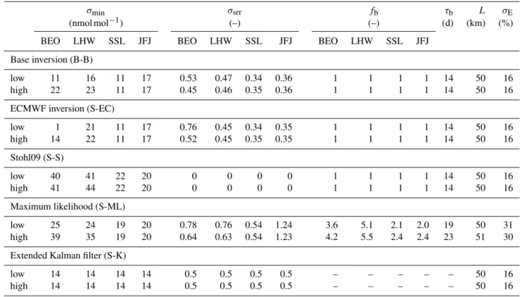
attribu-Table 3. Overview of parameters used for the construction of the uncertainty covariance matrices: contributions to model–observation uncertaintyσminandσsrr, baseline uncertainty factorfb, baseline correlation lengthτb, prior correlation lengthLand prior Swiss emission uncertaintyσE.
σmin σsrr fb τb L σE
(nmol mol−1) (–) (–) (d) (km) (%)
BEO LHW SSL JFJ BEO LHW SSL JFJ BEO LHW SSL JFJ
Base inversion (B-B)
low 11 16 11 17 0.53 0.47 0.34 0.36 1 1 1 1 14 50 16
high 22 23 11 17 0.45 0.46 0.35 0.36 1 1 1 1 14 50 16
ECMWF inversion (S-EC)
low 1 21 11 17 0.76 0.45 0.34 0.35 1 1 1 1 14 50 16
high 14 22 11 17 0.52 0.45 0.35 0.35 1 1 1 1 14 50 16
Stohl09 (S-S)
low 40 41 22 20 0 0 0 0 1 1 1 1 14 50 16
high 41 44 22 20 0 0 0 0 1 1 1 1 14 50 16
Maximum likelihood (S-ML)
low 25 24 19 20 0.78 0.76 0.54 1.24 3.6 5.1 2.1 2.0 19 50 31
high 39 35 19 20 0.64 0.63 0.54 1.23 4.2 5.5 2.4 2.4 23 51 30
Extended Kalman filter (S-K)
low 14 14 14 14 0.5 0.5 0.5 0.5 – – – – – 50 16
high 14 14 14 14 0.5 0.5 0.5 0.5 – – – – – 50 16
tion errors in the posterior emissions. Therefore, we explored two alternative methods that address certain shortcomings of our main approach. For example, there were times when the simulated smooth baseline was not able to follow apparent fast changes in the observed baseline signal. This was the case when the general advection direction towards Switzer-land quickly changed from west to east, with mole frac-tions often being considerably elevated during easterly ad-vection. At such transition times, use of the smooth baseline may lead to attribution errors in the emission field. Instead of a smooth baseline it would have been desirable to take the baseline directly from an unbiased state of a global-scale model, sampling the mole fractions at the FLEXPART parti-cle end points. However, such model output was not available for the investigation period at the time of the analysis.
The first alternative method (S-B1) was based on two base-line estimations – one for the eastern and one for the west-ern part of the inversion domain – which were combined using a weighted mean depending on the end points of the model particles (here 4 days before arrival at the site). Since the initial locations of the particles were available for every 3 h interval, this approach allows for more flexible variations of the simulated baseline signal. As in the standard baseline treatment, prior baseline mole fractions were taken from the REBS baseline at JFJ, applied here to both the eastern and western baselines. The second alternative baseline method
(S-B2) extended the approach to a three-dimensional grid of baseline mole fractions accounting not only for east–west but also for north–south and vertical gradients. Again, the initial positions of the model particles within the grid as obtained from each FLEXPART simulation were used to determine the baseline concentration at the site as a weighted average. Different from methods B and S-B1, however, only one com-mon set of gridded baseline mole fractions was estimated and applied to all sites. Only a very coarse (3×3×2) grid, cover-ing the inversion domain, with a 15-day temporal resolution was used in order to limit the size of the state vector. In the vertical, the grid was separated between heights 3000 m be-low and above ground level. The latter was chosen to ensure that average initial sensitivities were similar for both verti-cal layers. Prior baseline values in the upper vertiverti-cal layer were again taken from the REBS baseline at JFJ, whereas the lower layer was initialised with the REBS baseline at BEO. This ensures a negative vertical gradient in CH4 base-line mole fractions, since estimates for BEO were generally larger than those for JFJ.
3 Results
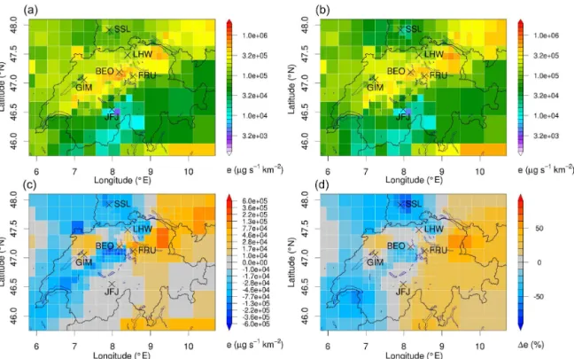
inver-Figure 2. (a) Prior and(b)posterior surface fluxes of CH4 in the base inversion and low particle release heights (B low).(c)Absolute and(d)relative (to prior) difference between posterior and prior emission fluxes. For(c)and(d)red (blue) colours indicate higher (lower) posterior than prior emissions.
sions highlighting the differences from the base case. Note that the base inversion does not necessarily represent the best inversion set-up and most likely or best estimate of the poste-rior emissions. Rather, it is used as a starting point to analyse the sensitivity to different inversion settings. Although there might be a best inversion set-up in the sense that its results are closest to the truth, this best set-up is not known (as little as the true emissions are known). The ML method applied as an alternative is an objective method to tune the free parame-ters of an inversion, but this does not necessarily correspond to the best set-up since it cannot account for potential biases arising from transport errors or the problem in representing the release height of the particles.
3.1 Base inversion
Average source sensitivities as calculated with FLEXPART-COSMO on the reduced grid are shown in Fig. 1 for the base inversion as the combined sensitivity of the four sites BEO, LHW, SSL, and JFJ. Source sensitivities were largest close to the sites and in general for the Swiss Plateau (see Oney et al., 2015, for a detailed discussion of source sensitivities of the CarboCount-CH sites). The pronounced south-west to north-east orientation of the maximal source sensitivities is a result of the flow channelling between the Alps and the Jura Mountains (Furger, 1990). South of the Alps and out-side Switzerland, source sensitivities quickly declined with
generally larger values for westerly compared with easterly directions. Source sensitivities towards the south-east were especially small, reflecting the shielding effect of the Alps.
In Switzerland prior emissions amounted to 178 Gg yr−1. After mapping the high-resolution emission data to the re-duced inversion grid (Fig. 2a) and applying Eq. (8), Swiss prior emissions were quantified at 183 Gg yr−1. The differ-ence of 2 % can be explained by mapping artefacts along the Swiss border, where inversion grid cells overlap with neigh-bouring countries, wrongly attributing some emissions from these to the Swiss total. The distribution of the prior emis-sions (Fig. 2a) in Switzerland clearly emphasises the domi-nant role of emissions from the agricultural sector. Emission maxima are located in the canton of Lucerne in close vicin-ity to BEO and in the north-eastern part of the country to-wards Lake Constance in the cantons of Thurgau and Saint Gallen. All these areas are characterised by intensive agri-culture with a focus on cattle farming. Emissions from the urban centres of Zurich, Basel, Bern and Geneva, in contrast, are not especially pronounced in the MAIOLICA inventory. Within the high Alpine area, and to a smaller degree within the Jura Mountains, MAIOLICA emissions are significantly smaller, but are large again in the north Italian Po Valley and also in south-western Germany.
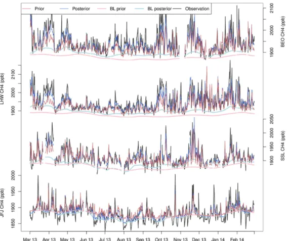
Figure 3.Observed (black) and simulated (prior: red; posterior: blue) CH4time series in the base inversion with low release heights (B low) at sites used in the inversion. Also given are the baseline mole fractions as used in the simulations (prior: light red; posterior: light blue). Note that theyaxes were scaled for each site separately. All data represent 3-hourly averages.
prior simulations were closely following the observed vari-ability, underlining the very good performance of the trans-port model. However, during some periods the prior simu-lations considerably underestimated the observed mole frac-tions. This was especially true for the BEO and LHW sites and a period in March/April as well as during episodes in October and November 2013. Some of the observed tempo-ral variability was common for all sites, suggesting an im-portant influence from large-scale weather systems, whereas at other times the signals from different sites were little cor-related. The two sites on the Swiss Plateau showed the most common behaviour, while, as expected, the high-altitude ob-servations at JFJ were most decoupled from the other obser-vations. Also as expected, peak mole fractions were larger for the sites closer to the emissions (BEO, LHW) and smaller for the higher-altitude sites (SSL and especially JFJ). The trans-port model captured this general tendency very well. Except for JFJ, prior baseline mole fractions (based on the JFJ REBS estimate) were smaller than most observed mole fractions.
The model’s skill considerably improved for the posterior simulations showing greater correlations and lower biases. The simulations more closely followed the observed vari-ability and the bias was reduced (Fig. 3). Partly, this was
achieved through changes in the baseline mole fractions. Pos-terior baselines were generally greater than the prior at the BEO, LHW and SSL sites, whereas they were lower than the prior at JFJ. Largest baseline increases occurred dur-ing extended periods of elevated CH4 (e.g. March 2013). These periods were characterised by easterly advection on the south-easterly side of high pressure systems with centres over north-western to central Europe. In these situations the limited model domain and the relatively short backward in-tegration time of 4 days were likely insufficient to capture all recent emission accumulation above the baseline. As a con-sequence, the inversion adjusted the baseline upward.
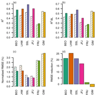
consider-Figure 4.Model performance parameters for simulated time series at all sites for the base inversion with low particle release heights (B low): prior (shaded) and posterior (filled).(a)Coefficient of de-termination (R2) for complete signal and(b)above-baseline signal, (c)normalised RMSE and(d)reduction of RMSE between prior and posterior. Note that the FRU and GIM sites were only used for validation but not in the inversion. All comparison statistics are based on 3-hourly averages.
ably increased for all sites used in the inversion (R2=0.58– 0.69) and slightly increased for FRU but slightly decreased for GIM. Improvements were seen both for the complete sig-nal as well as for the above-baseline sigsig-nal. The ranking be-tween the sites remained similar after the inversion.
An overall quality indicator, which not only accounts for the correlation but also for a correct representation of the amplitude of the variability, is the Taylor skill score (Taylor, 2001)
S= 4(1+R)
σf+σf−1 2
(1+R0)
, (15)
where R is the Pearson correlation coefficient and R0 the maximal attainable Pearson correlation of a “perfect” sim-ulation, which is still limited by factors such as observa-tion and representativeness uncertainty and was set to 0.9. σf =σm/σois the simulated standard deviation normalised by the observed standard deviation.Stakes the value of 1 for a perfect simulation, but would take a value of 0.65 for per-fectly correlated simulations that under/overestimate the ob-served variability by a factor of 2. The prior value ofσf was well below 1 for all sites (0.43 to 0.71), indicating generally underpredicted peak heights, but increased in the posterior simulation to values between 0.65 to 0.8, except for GIM,
where it remained at 0.44. Posterior values ofS for all sen-sitivity inversions and all sites are given in Table 4. For the base inversionSranged from 0.78 to 0.91 for the sites used in the inversion and was smaller for the sites FRU and GIM (0.77 and 0.50). Note, however, that for the latter two sites the baseline was not adjusted by the inversion, which may ex-plain part of the weaker posterior performance. In the case of GIM it is remarkable that the correlation was comparatively large but the normalised standard deviation was very small. This may indicate that the general transport to the site was well captured by the model (correlation), but that either lo-cal boundary layer heights or lolo-cal emissions were overesti-mated or underestioveresti-mated, respectively, so that the model was not able to simulate the observed amplitudes correctly. Taylor skill scores were very similar for posterior simulations of the base inversion using the high particle releases (B high in Ta-ble 4). Also, the prior simulation’s performance was similar for low and high release heights, with lower release heights usually performing slightly better in terms of amplitude of the simulated variability and higher release heights showing slightly improved correlations. No clear preference for the lower or higher release height could be deduced from these results.
As an additional validation parameter the RMSE and its reduction from prior to posterior simulations are shown in Fig. 4c and d. For sites used in the inversion the prior RMSE was between 20 and 40 nmol mol−1and decreased by 15 to 25 % in the posterior simulations. For the near-surface sites FRU and GIM the RMSE did not significantly decrease af-ter the inversion. At both sites simulated mole fractions were smaller than observed, especially at GIM. Even when using only afternoon values and when filtering for wind conditions with possibly large local influences (as done here), the trans-port model was not able to reproduce the amplitude of the ob-served variability at these sites. A reason for this poor model performance in FRU is most likely the inlet height being very close to the surface and the associated high sensitivity to lo-cal emissions that cannot be captured at the resolution of the transport model. In GIM local emissions or mismatches in the local boundary layer height seem to be the main problem since the timing of the temporal variability was captured very well. The effect of including the sites GIM and FRU in the inversion is further discussed in Sect. 3.7.
We used observations from sites in more complex terrain and closer to emission sources than used in other regional-scale inversion studies of CH4 surface fluxes for the Euro-pean and East Asian domain (Bergamaschi et al., 2015; Man-ning et al., 2011; Thompson et al., 2015). This should result in more complex variability at the sites. Nevertheless, our model performance parameters are well within the range re-ported previously by the above studies.
Table 4.Overview of results of sensitivity inversions.EAandEBare the total Swiss CH4prior and posterior emissions (Gg yr−1), respec-tively, andSis the posterior Taylor skill score for the individual sites. The settings of the sensitivity inversions are given in Table 2.
Inversion Emissions Skill score (S)
priorEA posteriorEB BEO LHW SSL JFJ FRU GIM
B low 183.0±29.3 179.0±7.0 0.83 0.89 0.91 0.78 0.77 0.50
B high 183.0±29.3 195.0±7.3 0.84 0.86 0.91 0.78 0.74 0.51
S-V low 183.0±29.3 185.9±6.5 0.84 0.89 0.91 0.77 0.77 0.51
S-V high 183.0±29.3 197.3±6.7 0.85 0.86 0.91 0.78 0.75 0.53
S-K low 179.6±28.7 193.1±13 0.92 0.94 0.94 0.84 – –
S-K high 179.6±28.7 216.7±14 0.93 0.95 0.94 0.85 – –
S-EC low 184.4±28.0 171.1±8.0 0.79 0.87 0.91 0.77 0.74 0.29
S-EC high 184.5±29.0 182.1±7.6 0.88 0.87 0.92 0.77 0.74 0.31
S-T low 188.1±30.1 180.3±7.2 0.82 0.89 0.91 0.78 0.74 0.44
S-T high 187.7±29.7 199.1±7.4 0.83 0.87 0.91 0.78 0.69 0.46
S-E low 228.2±36.5 184.3±7.9 0.84 0.89 0.90 0.77 0.75 0.43
S-E high 227.4±36.4 207.1±7.9 0.83 0.88 0.90 0.77 0.69 0.46
S-S low 183.3±29.3 169.3±7.5 0.79 0.84 0.89 0.77 0.70 0.39
S-S high 183.3±29.3 197.6±8.0 0.81 0.84 0.89 0.77 0.70 0.51
S-ML low 183.0±37.3 158.4±13 0.84 0.92 0.90 0.78 0.73 0.44
S-ML high 183.0±65.6 168.7±13 0.85 0.91 0.89 0.78 0.66 0.44
S-O1 low 184.9±29.2 183.3±10 0.85 0.83 0.84 0.62 0.78 0.40
S-O1 high 184.6±29.5 200.8±11 0.87 0.81 0.84 0.63 0.78 0.38
S-O2 low 185.8±29.7 214.3±11 0.77 0.90 0.83 0.66 0.77 0.57
S-O2 high 184.5±29.6 229.6±11 0.75 0.88 0.82 0.66 0.76 0.64
S-O3 low 183.3±29.3 198.5±7.9 0.85 0.91 0.84 0.66 0.79 0.49
S-O3 high 183.5±29.4 221.3±8.3 0.86 0.89 0.83 0.66 0.78 0.51
S-O4 low 183.3±28.3 191.2±6.2 0.84 0.90 0.91 0.78 0.82 0.46
S-O4 high 183.3±29.2 207.7±6.5 0.85 0.88 0.91 0.79 0.85 0.48
S-O5 low 181.9±29.1 208.8±6.0 0.84 0.90 0.92 0.79 0.83 0.66
S-O5 high 181.9±29.1 224.3±6.1 0.85 0.88 0.91 0.79 0.85 0.69
S-B1 low 183.0±29.3 194.0±6.9 0.83 0.89 0.92 0.79 0.77 0.49
S-B1 high 183.0±29.3 211.7±7.2 0.84 0.87 0.92 0.79 0.74 0.51
S-B2 low 183.0±29.3 195.1±6.9 0.88 0.89 0.92 0.83 0.82 0.62
S-B2 high 183.0±29.3 223.6±6.9 0.88 0.88 0.92 0.83 0.75 0.69
large prior emissions from agriculture, reductions were in the order of 25 %. Further reductions were estimated east of the site LHW in the canton of Thurgau (please refer to Fig. S1 for a map of the Swiss cantons) and in large parts of western Switzerland. In contrast, larger than prior emissions were ob-tained for north-eastern Switzerland in the cantons of Saint Gallen and Appenzell and also beyond the border in south-western Bavaria. Emissions in northern Italy were increased but due to the weak sensitivity for this region these posterior results are subject to larger uncertainties than those on the Swiss Plateau. Relative emission increases (Fig. 2d) of up to 30 % were detected for the Appenzell region and the border-ing Vorarlberg region in Austria. However, relative emission reductions appeared for the southern Black Forest. Similar patterns emerged for the base inversion when using the high release heights (see Fig. S3 in the Supplement), but posterior emissions were generally larger in this case.
In this base inversion Swiss total emissions were estimated at 179±7 Gg yr−1(1σ) and 195.0±7.3 Gg yr−1for the low
and high particle release heights, respectively. Both values are not significantly (two-sided Welcht test) different from their prior value, indicating a high level of consistency be-tween the bottom-up estimate of the MAIOLICA inventory and our top-down estimate. Furthermore, analytical uncer-tainties of the posterior were considerably reduced by about 75 %. However, the difference ±15 Gg yr−1 in total Swiss emissions resulting from the choice of the particle release height suggests a relatively large additional contribution to the overall uncertainty due to the inversion set-up, which is not included in the analytical uncertainty.
Figure 5.Uncertainty reduction between prior and posterior fluxes given in % relative to prior uncertainty (1−σB/σA) for the base
inversion with low particle release height.
around and west of BEO, where emission reductions were also the largest. Uncertainty reductions were smaller for the area east of LHW, where considerable emission reductions were also established. For north-eastern Switzerland, where the inversion produced large emission increases, uncertainty reductions were relatively small. The associated emission creases are thus less well constrained, which in turn may in-dicate temporally variable emissions or increased transport uncertainties for the associated flow direction.
3.2 Seasonal cycle
When allowing seasonal variability of the emission fluxes (S-V), distinct differences between the seasons are visible, although no seasonal variability was included in the prior (Figs. 6 and S4 in the Supplement). Wintertime posterior emissions were strongly reduced especially in agricultural ar-eas. Posterior emissions during the other seasons tended to be slightly larger than their prior values.
Also, the estimated emission patterns changed from sea-son to seasea-son. In spring and summer increased posterior emissions were estimated for eastern Switzerland, the canton of Lucerne (around BEO) and generally the pre-Alpine area, whereas there was a tendency for smaller than prior emis-sions in western Switzerland. The strong increase around the station FRU (not used in the inversion) is consistent with the observation that the posterior model performance for the site FRU was considerably enhanced compared to the prior simulation. Performance was also enhanced compared to the posterior simulation of the base inversion both in terms of correlation and RMSE reduction, although Taylor skill scores were similar in both inversions (see Table 4). How-ever, during autumn higher than prior emissions were present in north-western and eastern Switzerland, and for small areas south of BEO and east of LHW posterior emissions were be-low prior estimates.
For the low model release height, total Swiss emission rates were smallest during winter (152.2±9.7 Gg yr−1) but
were relatively similar and close to the prior estimates dur-ing the other seasons (206.5±12, 182.1±13, and 202.7± 11 Gg yr−1 for spring, summer and autumn, respectively). The annual total Swiss emissions for S-V were 185.9± 6.5 Gg yr−1, very close to those of the base inversion. Winter-time emission rates were 18 % smaller than the annual mean. For the high model release heights, a similar but less pro-nounced annual cycle was derived, which featured total an-nual emissions of 197±7 Gg yr−1and wintertime emission rates of 171±10 Gg yr−1(13 % lower than annual mean). 3.3 Extended Kalman filter inversion
The extended Kalman filter inversion using low particle re-lease heights (S-K low) yielded similar annual mean poste-rior emissions as the base inversion (Figs. 7 and S5 in the Supplement). Several features of the posterior emission dif-ferences obtained by the base inversion are also visible in the extKF inversion: reductions west of BEO, increases in north-eastern Switzerland, small changes in the Alpine area, small increase in the region close to GIM (shifted south-westerly as compared to base inversion). No emission reductions were, however, deduced for the area east of LHW. Overall the pos-terior model performance using the extKF inversion was su-perior (S between 0.84 and 0.95) compared to the base in-version (Table 4), which is most likely related to the time-variable posterior emission field and to a smaller degree to the different treatment of baseline mole fractions.
Figure 6.Absolute difference between posterior minus prior emission fluxes for seasonal inversion.(a)December, January, and February; (b)March, April, and May;(c)June, July, and August; and(d)September, October, and November.
Figure 7.Absolute difference between posterior minus prior emis-sion fluxes as obtained from extended Kalman filter inveremis-sion with low particle releases.
3.4 Influence of transport model
In the sensitivity case S-EC the source sensitivities were derived from ECMWF instead of COSMO (see Sect. 2.2). On the one hand, FLEXPART-ECMWF may be less suitable to resolve the complex flow in the Swiss domain due to its coarser horizontal resolution. On the other hand, FLEXPART-ECMWF is a well-validated model code and has been widely used for inverse mod-elling (e.g. Stohl et al., 2009; Thompson and Stohl, 2014;
Thompson et al., 2015). Using the same inversion settings, FLEXPART-ECMWF simulations yielded generally similar posterior emissions as the base inversion (Figs. 8 and S6 in the Supplement). Common features were again the decrease west of BEO and east of LHW and the increase in north-eastern Switzerland with respect to the prior emissions. In contrast to the base inversion, large emission reductions were also assigned to most of the western part of the country to-wards Lake Geneva. For the low release height, the model performance at the observation sites was only slightly lower compared to the base inversion as indicated by the poste-rior Taylor skill scores (Table 4). In contrast, posteposte-rior Taylor skill scores were slightly larger in the high release case than in the base inversion. An exception was the GIM site, for which skill scores were strongly reduced using FLEXPART-ECMWF. This may reflect the growing inability of a coarser transport model to simulate the local CH4contribution to the site.
Figure 8. (a)Absolute difference between posterior minus prior emission fluxes for S-EC with low particle release height.(b)Uncertainty reduction between prior and posterior fluxes given in % relative to prior uncertainty (1−σB/σA).
than in the base inversion. One possible explanation may be the coarser and, hence, potentially less dispersive behaviour of FLEXPART-ECMWF. Mesoscale flow patterns in com-plex terrain may contribute to effective dispersion (Rotach et al., 2013). The coarser resolution of FLEXPART-ECMWF likely results in larger under-representation of mesoscale flow in the complex Swiss terrain.
3.5 Influence of prior emissions
Two additional spatially explicit sets of prior emissions were used to explore the effect of the prior emissions on the in-version results. The sensitivity run based on EDGAR (S-E) starts off from considerably larger prior emissions for Switzerland (228 Gg yr−1) and also deviates strongly in the spatial allocation of these emissions, putting more empha-sis on the population centres than the MAIOLICA inventory (Hiller et al., 2014a). This can be traced back to EDGARv4.2 containing about 25 Gg yr−1 larger emissions from the gas distribution network (IPCC category 1B2: fugitive emis-sions from oil and gas; 32 vs. 8 Gg yr−1 in MAIOLICA), while other emission categories are similar. However,the re-maining emissions are also more closely following the dis-tribution of population density when compared with the MAIOLICA inventory, which is due to less detailed geo-graphical information in the EDGARv4.2 inventory (Hiller et al., 2014a). Differences between the TNO inventory (S-T) and the MAIOLICA inventory are more subtle and amount to only 5 Gg yr−1for the Swiss total.
In all three inversions (B, S-E and S-T) posterior emissions were very similar both in their distribution (see Figs. S3, S7, S8 in the Supplement) and the national total. The latter only differed by 5 Gg yr−1for S-T and 10 Gg yr−1for S-E despite the fact that prior emissions were 45 Gg yr−1larger in the lat-ter (Table 4). This indicates that the poslat-terior emissions were well constrained by the observations and not solely governed by the prior emissions for which relatively small uncertain-ties were assigned. The strong posterior emission increase in north-eastern Switzerland was also prominent in S-E. The
posterior to prior differences for S-E showed a strong emis-sion reduction in the larger urban areas (mainly Basel and Zurich, but also Lucerne, Bern and Geneva), suggesting that the strong attribution of emissions to urban centres in the EDGAR inventory is unrealistic (Fig. 9a). In contrast to the base inversion, uncertainty reductions in the S-E case were also large for the urban areas (Fig. 9b), lending credibility to the associated emission reductions.
3.6 Influence of uncertainty covariance treatment The inversion results using the model–observation uncer-tainty as estimated by the method of Stohl et al. (2009) (S-S) were smaller than in the base inversion in the low release case but differed only slightly in the high release case (see Table 4). In S-S an almost constant value (see Sect. 2.4) was given to the model–observation uncertainty of each site, while in the base inversion uncertainties tended to be larger for large above-baseline mole fractions. However, model un-certainties were mostly smaller for the base inversion except for 10 to 20 % of the observations in the “low” and less than 10 % in the “high” release case. Despite these differences in the applied model uncertainty, the distribution of posterior fluxes was similar to that of the base inversion, with two ex-ceptions: emission reductions were more pronounced in the area west of BEO and east of LHW in the S-S case and ad-ditional reduction occurred around the BEO site itself (see Fig. S9 in the Supplement). The distinct posterior increase in north-eastern Switzerland was also present in S-S.