Testing the long-run implications of the expectation hypothesis using cointegration techniques with structural change

T

T

L

-R

I

O

T

E

H

U

C

T

W

S

C

P

L.

V

P

Janeiro

de 2009

T

T

e

e

x

x

t

t

o

o

s

s

p

p

a

a

r

r

a

a

D

D

i

i

s

s

c

c

u

u

s

s

s

s

ã

ã

o

o

TEXTO PARA DISCUSSÃO 175 • JANEIRO DE 2009 • 1

Os artigos dos Textos para Discussão da Escola de Economia de São Paulo da Fundação Getulio Vargas são de inteira responsabilidade dos autores e não refletem necessariamente a opinião da

FGV-EESP. É permitida a reprodução total ou parcial dos artigos, desde que creditada a fonte.

Escola de Economia de São Paulo da Fundação Getulio Vargas FGV-EESP

“Testing the long-run implications of the expectation hypothesis using cointegration techniques with structural change”.

Emerson Fernandes Marçal

Universidade Presbiteriana Mackenzie e IE-UNICAMP R. Conselheiro Brotero 1030, apt 33

01232-010, São Paulo, S.P. Tel: (011) 3824-9205 Fax: (011) 3663-4345 efmarcal@gmail.com

Pedro Luiz Valls Pereira EESP-FGV

Rua Itapeva 474 room 1202 01332-000, São Paulo. S.P. Tel: (011) 3281-3726 Fax: (011) 3281-3357 pedro.valls@fgv.br

Omar Abbara IMECC-UNICAMP Caixa Postal 6065

13083-859, Campinas, S.P. muhieddine@gmail.com

Abstract:

1

qui-squared distribution. The results of the paper show evidence in favor of the long run implications of the expectation hypothesis for Brazil.

Key-words: Term structure, cointegration, structural change JEL codes: C32; C52; G14

1

Introduction:

A recent effort has been done to test the expectation hypothesis for Brazilian data. Although this research is in its early stages for Brazil, there is a vast literature about this theme for other countries. (Cuthbertson and Nitzsche (2005))

This paper aims to investigate whether or not multivariate cointegration models with structural change can better describe the term structure of interest rate data for the period from 1995 to 2006. The work uses the Generalized Reduced Rank Technique recently developed by Hansen (2003) to estimate cointegrated process with structural change. Under this framework the number of cointegration relations and the number and the moments of the structural change are assumed to be known. This allows testing hypothesis about the parameters in all regimes and evaluating whether or not there is structural change. It’s also done an effort to control the possible non-stationarity of volatility by using the results of Boswijk and Zu (2005). As far as the authors know this has not been done in the literature for Brazil.

The paper is organized in the following questions. The first section discusses the expectation hypothesis. The second section presents the Generalized Reduced Rank technique and how to correct for heterocedasticity under this framework. The third section the results of the estimated models are shown and discussed. The next section a comparison with the literature is done. Finally the main conclusions are stated.

2

Expectation Hypothesis: What is?

Define m t

R as the logarithmic of annualized return paid by a m period long run bond

and by n t

R , the logarithmic of the annualized return paid by a n period short run bond with

m < n then the spread (m,n) Sm,n can be defined as n t m t R

R − .

2

eq. 1:

( )

n m t n

in t n

n t n

in t n t t m

t k E R R R R T

R = 1 [ + + + +2 +...+ + ]+ ,

where Et denotes the expectation formed in instant t, k = (m/n), i = 1,2,..,k and

,

m n t

T the premium for the agents who decides for a long term strategy.

The investor can decide between two strategies. In the first he holds a bond of

maturity m and obtains an annualized return of m t

R . The other strategy consists in buying

bonds of maturity m during (m/n) successive periods. In equilibrium the equation (eq. 1) must hold if the agents arbitrate the difference in two relations corrected for the risk premium and if the expectations are rational. This is called the expectation hypothesis. The discussion about the determinants of term premium started long ago. Authors like Keynes (1930) and Hicks (1946) have discussed its determinants. A recent survey was done by Shiller (1990).

Cuthbertson and Nitzsche (2005) pages 494 to 498 show the following typology to model the term risk premium:

I) Pure Expectation Hypothesis: the term premium is assumed to be constant and equals zeros for all maturities.

II) Constant Premium Expectation Hypothesis: The term premium differs from zero and it is equal for all maturities;

III) Liquidity Preference or Growing Term premium: The term premium is constant throughout the time and it’s bigger for longer spreads;

IV) Time Varying Risk Premium: the term premium varies throughout the time;

V) Market Segmentation: The value of the asset depends in some way of its stock level and this influences the spreads;

VI) Preferred Habitat Theory: Bond that matures at the same date should be reasonably close substitutes and, hence, have similar term premium.

3

under certain circumstances. The model V contains possible explanation for the failure of the expectation hypothesis in its stronger versions. The model VI is a very skeptical approach for the expectation hypothesis.

The expectation hypothesis can also be stated as the following form.

eq. 2: mn

t k i n in t n t n t m

t E R T

k i R R , 1 1 ) ( ) 1 ( − ∆ + = −

∑

The eq. 2 is the starting point for the most of the test of the so-called expectation hypothesis. One can note that if the short interest rate following an integrated process of order one and the term premium is time varying but stationary, then the spreads must stationary.

3

Econometric Methodology:

In this section it will be discussed the econometric techniques used in the paper. The generalized reduced rank regression is briefly discussed and it will be shown how it can be used to estimate cointegrated models with structural change. This part of the paper is based mainly in Hansen (2003).

3.1

Estimating a VAR with structural change:

Hansen (2003) generalizes the model proposed by Johansen (1988):

eq. 3 T m ,m , j ,T , t j j j j

j _{k k t}

< = = + + Φ + ∆ Γ + + ∆ Γ = ∆ − − ... 1 ... 1 ) ( ) ( ) ( ) ( ... )

( _{α β}' _ε

1 t t t t 1

t X X D X

X

where εt are random errors with Ω(j) as the covariance matrix and j denotes the regime.

The first regime starts at t=0 and ends at t=T1-1. The second regime starts at t=T1 and ends at t=T2-1 and so on. It’s assumed that there are m different regimes.

4 eq. 4 1 0 ) 1 ( 1 1 1 ,..., 1 1 ... 1 ) ( 1 ... 1 ) ( 1 ... 1 ) ( 0 1 , , , , 1 , 1 , , , 1 , 1 , , , 1 , 1 + ≡ ≡ − ≤ ≤ ≡ − = Ω + + Ω = Ω Φ + + Φ = Φ Γ + + Γ = Γ − T T T T t T k i j j j m j j t j t m i m t i t m i m t i t m i m t i i

By using the following notation: Z_ot =∆X_t , (1 ,...,1 , ' 1)' '

1 , 1

1t = tXt− mtXt−

Z , )' , ,..., ( ~ ' ' ' 1

2t Xt Xt k Dt

Z = ∆ ₋ ∆ ₋ ,

                = − m m B β β β β 0 ... 0 0 0 ... 0 0 ... ... 0 ... ... 0 0 0 ... 0 1 2 1 ) ,...,

( _{1 m}

A= α α ,

) ,..., (ψ₁ ψ₁

=

C and ψ_j =(Γ_j,1,...,Γ_j,k−1,Φ_j).

The eq. 1 can be rewritten as

eq. 5 Z_0t =AB'Z_1t +CZ_2t +ε_t

The problem consists in finding an estimator for A, B and C. This can be done by using the GRRR.

3.1.1 Generalized Reduced Rank Regression (GRRR):

Hansen (2003) show how to estimate the process described in eq. 5. In order to do this he uses the vec operator and defines two matrices H and G::

eq. 6 vec(B)=Hϕ+h

where H is known, φ

, contains the free parameters and h is a tool to normalize or

identifies the parameters A and B. eq. 7 vec(A,C)=Gψ

where G is known and, ψ, contains the free parameters.

5 eq. 8

1

' '

1 1 1 2 1

' '

1 _{2 1 2 2}

1 ' ' 1 2 1

ˆ_' ˆ ˆ_'

ˆ ˆ ˆ

( , ) ' ( )

ˆ

ˆ ˆ

' ( ( ) ( , ))

T

t t t t

t _{t t t t}

T

ot t t t

B Z Z B B Z Z

vec A C G G t G

Z Z B Z Z

G vec t Z Z B Z

− − = − =         

=  ⊗ Ω ×

   _{ } _    Ω

∑

∑

1 1 '

1 0 2 1

1 1

ˆ ˆ

ˆ ˆ

( ) ' ( ' ( ) )

ˆ ˆ ˆ ˆ ˆ ˆ

' ' ( ( ) ' ( ) ) ( ' ( ) ) t T t t t T T

t t t t

t t

vec B H H A t A Z Z H

H H vec Z Z CZ t A A t A Z Z h h

− − = − − = =  

=  Ω ⊗  ×

 

 

− Ω − Ω ⊗ +

 

 

∑

∑

∑

eq. 10

∑

+ = − − − − = Ω j j T T t t t j j T T j 1 1 1 1 'ˆ ˆ ) ( ) (

ˆ _εε

eq. 11 εˆt =Z0_t −AˆBˆ'Z1_t +CˆZ2_t

This equation must be used iteratively. The analysts starts the routine with a good guess for A, C and Ω(t) and then obtains an estimator for B. Then another estimator for B

and Ω(t)can be obtained. The process must continue until convergence and the maximum

likelihood estimator are obtained (see Hansen (2003) for details).

The algorithm can also be used to estimate the model if one assumes that variance and covariance of the errors are known (or estimated previously). The algorithm uses only equations 8 and 9. In this case Ω(t) is estimated using the Dynamic Conditional

Correlation Model of Tse & Tsui (2002) and it is this approach that is used in order to control the heteroscedasticity in the model.

3.2

Description of the estimate models:

6

part of this paper. It is used models with 4 regimes. With the exception of the variance and covariance matrix of the errors, all other parameters can be made different within the regimes.1

The starting point of the analysis is the following VECM:

eq. 12 ∆ =Γ∆ − +Γ∆ − +α(t)(β (t) − +ρ(t))+εt

' 2

2

1 t t 1

t 1

t X X X

X 2

εt ~N(0,Ω(t)) [ ]'

360 180 90 60 30

i i i i i

=

t

X

3.3

Data base description:

The data were collected from Risktech web page (www.risktech.com.br) for

different vertices. The frequency of the data is monthly and the data corresponds to last working day of the month. The vertices were chosen due to liquidity constrains for 30, 60, 90, 180 e 360 days.

Figure 1 shows the evolution of all interest rate for the whole sample. Some periods, particular in the beginning of the sample has huge instability. This is due to the effects of financial crisis in Asia, Russia. Brazilian economy had worked with an almost fixed exchange rate regime that generates great volatility in interest rates. After 1999 the interest rates have smoother movements. There is also a tendency of interest rate falling in long run.

Figure 1: Taxa de Juros de 30, 60, 90, 180 e 360 dias.

1 _{It is possible to work with different error variances, allowing for heteroscedasticity. Since the sample}

is not big enough to accommodate all this heavy structure. It must be noted that a time varying short structure in the models allow for different unconditional variances.

2_where ( )

t

7

1996 1997 1998 1999 2000 2001 2002 2003 2004 2005 2006 2007

0.15 0.20 0.25 0.30 0.35

Li30 Li90 Li360

Li60 Li180

3.4

Report of the estimation results:

Figure 2: shows the evolution of the spreads for different vertices. There is great volatility from the beginning of the sample until 1998. After the changes in exchange rate regime in January of 1999, the spreads are less volatile and with an apparent large memory.

Figure 2: Spreads for different maturities.

1996 1997 1998 1999 2000 2001 2002 2003 2004 2005 2006 2007

-0.02 -0.01 0.00 0.01 0.02 0.03

S60_30

S180_90 S90_30 S360_180

8

• regime 1: from 1995:1 to 1997:9 – (macroeconomics stabilization process);

• regime 2: from 1997:9 to 1998:12 – (Asian Crisis);

• regime 3: from 1999:1 to 2006:12 (floating exchange rate era and second Cardoso administration and first Lula administration);

The following models were estimated:

• Model 01: Unrestricted with three complete different regimes.

• Model 02:

                    − − − − = = = 4 3 2 1 ' ' ' 1 0 0 0 1 1 0 0 0 1 1 0 0 0 0 1 0 0 1 1 ) 3 ( ) 2 ( ) 1 ( ρ ρ ρ ρ β β β

• Model 03: Restrictions imposed in model 02 plus α(1)=α(2)=α(3)=α. There is no structural change in first moment of the process.

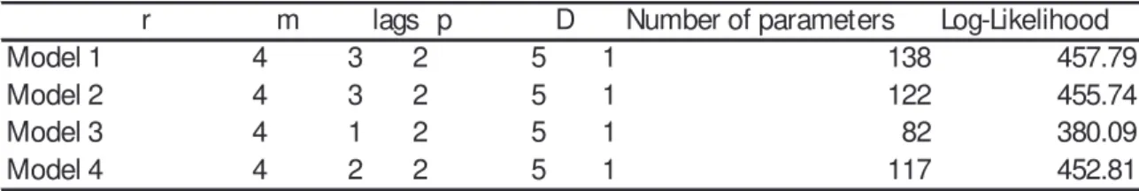
Table 1: Likelihood ratio test for proposed simplifications.

r m lags p D Number of parameters Log-Likelihood

Model 1 4 3 2 5 1 138 457.79

Model 2 4 3 2 5 1 122 455.74

Model 3 4 1 2 5 1 82 380.09

Model 4 4 2 2 5 1 117 452.81

In Table 2 the simplifications from the general model are tested. The hypothesis the spreads and the average term premium does not differs significantly in the three regimes is not rejected from the data (line 1). The hypothesis that there is no structural change in first moment of the process is strongly rejected from the data (line 3).

Then using this structure it is possible to document the existence of three different regimes. The first starts in 1995:1 and ends in 1997:9. The second starts in 1997:10 and ends in 1998:12. The third regime starts in 1999:1 and lasts until the end of the sample.

9

that results in zero (a’* α(t)=0). If α is constant in all regimes then the common trends are

the same in all regimes. Suppose that this structure is correct α(t)= α∗∗ρ(t) where α∗ is a p

x r matrix and ρ(t) is a r x r matrix, then it’s possible to find a matrix a that satisfies the

restrictions a’* α(t)= a’* α∗_∗ρ(t)=0.

The model under this restriction can be estimated using GRRR and a likelihood ratio test can be formulated to test the validity of this hypothesis. Then the hypothesis that the common trends remain the same during the period of 1997:9 to 2006:12 is not rejected by the data (line 3). Despite the fact that there is evidence of structural change under the whole period, the change does not affected the long run implications of the expectation hypothesis. The spreads are found to be stationary and the factors that drive the interest rate remains intact during the whole sample.

The evidence of a changing structure can be rationalized under the McCallum (1994) framework. In this paper he had shown that the spreads can have memory if the risk premium evolves as a process that has memory (as an autoregressive process for example). A change in the risk pattern or the rules followed by central bank can imply in a relation between spreads and first difference of short rates that change throughout the time.

To sum up the evidence in this paper is favorable of the expectation hypothesis if it’s assumed a time variant risk premium. However it must be noted that not all the implications of the expectation hypothesis is tested. For example, if the expectation hypothesis holds under McCallum (1994) framework the spreads can be approximated by an autoregressive process but only the past value of the spreads can help to predict the current values of the spreads. (See for example Serna and Arribas (2006) and Gallmeyer, Hollifield and Zin (2005))

Table 2: Likelihood ratio test for proposed simplifications.

Ha: Ho: Likelihood

Ratio

Degree of freedom

p-value

Line 1 Model 1 Model 2 4.10 16 99.87%

Line 2 Model 1 Model 3 155.41 21 0.00%

10

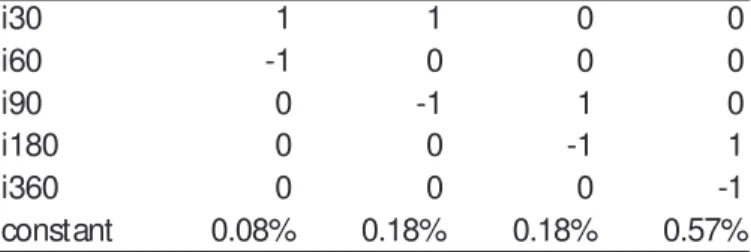
Table 3: Cointegrated vectors estimated from the best model.

i30 1 1 0 0

i60 -1 0 0 0

i90 0 -1 1 0

i180 0 0 -1 1

i360 0 0 0 -1

constant 0.08% 0.18% 0.18% 0.57%

The poor performance of expectation hypothesis for Brazilian data reported in the literature is related to non-modeled conditional heterocedasticity. In terms of long run implications of the expectations hypothesis it was not possible to reject that the short spreads are stationary in all regime: spread (60, 30), spread (90, 30). The spread (180, 90) and spread (360, 180) are found to be stationary in the whole sample. In the first sample the hypothesis that these spreads are stationary are rejected. One possible tentative explanation to this fact is the conjunction of the effects of Mexican crisis and stabilization process in Brazilian economy started in 1994 on term structure did not encourage the agents to arbitrage the difference between short and long run rates due to risk considerations (expected devaluation of Brazilian currency and inflation concern). The estimated cointegration vectors are reported in Table 4.

4

Comparison with other papers:

Hansen (2003) implemented the same test for American data. The author divides the sample in 3 periods. There are some differences from this work. He controls for heteroscedasticity but imposes the same short-run structure to all regimes. It is not possible to reject the hypothesis of stationary of the spreads. The constant risk premium hypothesis across the sub-samples is rejected. The hypothesis that the common trend remains the same is not rejected.

11

The study of the term structure for Brazilian data is at its early stages. The following works uses cointegration techniques to test the expectation hypothesis: Brito, Guillen and Duarte (2004), Lima and Isler (2003), Marçal (2004) and Marçal and Valls Pereira (2007). Just Marçal (2004), Marçal and Valls Pereira (2007) tries to model more than two vertices simultaneously using a cointegrated VAR. They have found evidence of cointegration but the evidence of stationary for longer spreads is weak.

Brito, Guillen and Duarte (2004) use cointegration techniques to test the expectation hypothesis. They have worked with daily data from 01/07/1996 to 31/12/2001. The cointegration hypothesis is tested using Johansen cointegration test. The authors conclude that the cointegration vector is equal to the spreads and this validates the expectation hypothesis. The frequency of the data is daily while the frequency of this work is monthly. In high frequency data it’s more likely to find some sort of conditional heteroscedasticity. If some conditions are not satisfied the trace and maximum eigenvalue statistics cannot be used (Rahbek, Hansen and Dennis (2002)). Under monthly data the conditional heteroscedasticity can be seen as a minor problem. But the fact is that the result of this work is different from their work.

Lima and Isler (2003) uses the ADF and Phillips-Perron test to evaluate whether or not the spreads are stationary. They have used monthly data from January of 1995 to December of 2001. They have obtained evidence in favour of no unit root in spreads (Lima and Isler (2003), p. 886). These results are confirmed by bivariate cointegration tests Lima and Isler (2003), pages. 888 e 889) applied to short and long interest rate. No effort to build up a VEC was done.

12

5

Conclusion:

This work investigates the evidence of structural change in Data Generator Process of Brazilian term structure of interest rate data. It is documented the presence of 3 regimes. The first lasts from 1995:1 to 1997:9. The second lasts from 1997:10 to 1998:12. The third lasts from 1999:1 to the end of the sample (2006:12).

The cointegration vector equals the spreads in all regimes and the common trends remains unchanged despite the evidence of structural change. Future studies of term structure using Brazilian data should be aware of the differences among the three periods and particularly with the data sooner after the Real Plan (particularly before 1997). As there is the ‘1979-1982 data problem’ in American term structure of interest rate (Seo (2003), Hansen (2003) and Cuthbertson and Nitzsche (2005)), it seems reasonable to state that there is a similar data problem for Brazilian data (post Real Plan and Asian Crisis data - 1995:1 to 1998:12) but the long-run implications of expectation hypothesis is satisfied.

6

References:

Boswijk, H. Peter, and Y. Zu, 2005, Testing for Cointegration with Nonstationary Volatility, (Tinbergen Institute & Amsterdam School of Economics).

Brito, R. D., O. T. C. Guillen, and A. J. M. Duarte, 2004, Overreaction of yield spreads and movements of Brazilian interest rate, Revista de Econometria 24, 1-55.

Campbell, J, and R. J. Shiller, 1991, Yield Spreads and Interest Rate Movements: A Bird's Eye View, Review of Economic Studies 58, 419-514.

Cuthbertson, Keith, and Dirk Nitzsche, 2005. Quantitative Financial Economics (John

Wiley & Sons Ltd., West Sussex).

Gallmeyer, Michael F., Burton Hollifield, and Stanley E. Zin, 2005, Taylor Rules, McCallum Rules and the Term Structure of Interest Rates, NBER Working Paper (NBER, Cambridge).

Gonzalo, J., and C. W. J. Granger, 1995, Estimation of Common Long-Memory Components in Cointegrated Systems, Journal of business and Economics Statistics

13.

Hansen, Peter Reinhard, 2003, Structural changes in the cointegrated vector autoregressive model, Journal of Econometrics 114, 261-295.

Hicks, John, 1946. Value and Capital (Oxford University Press, Oxford).

Johansen, Soren, 1988, Statistical Analysis of cointegration vectors, Journal of Economic Dynamics and Control 12, 231-254.

Johansen, Soren, and Anders Rygh Swensen, 1999, Testing exact rational expectations in cointegrated vector autoregressive models, Journal of Econometrics 93, 73-91.

13

Expectations in Cointegrated Vector Autoregressive Models:Restricted Drift Terms, Discussion Papers 348 (University of Oslo, Oslo).

Keynes, J. M., 1930. Treatise on Money.

Lima, A. M., and J. V. Isler, 2003, A hipótese das expectativas na estrutura a termo da taxa de juros no Brasil: Uma aplicação de modelos a valor presente, Revista Brasileira de Economia 57.

Marçal, E. F., 2004, Ensaios sobre eficiência, cointegração, componentes comuns, não linearidades na variância nos mercados financeiros: um estudo da estrutura a termo das taxas de juros e da volatilidade de títulos da dívida soberana., Departamento de Economia (Univesidade de São Paulo, São Paulo).

Marçal, E. F., and P. L. Valls Pereira, 2007, A Estrutura a Termo das Taxas de Juros no Brasil: testando a hipóteses de Expectativas, Pesquisa e Planejamento Econômico

37, 113-147.

McCallum, B. T., 1994, Monetary Policy and the Term Structure of Interest Rate,

Economic Quartely 91, 1-21.

Rahbek, Anders, Ernst Hansen, and Jonathan G. Dennis, 2002, ARCH Innovation and their impact on Cointegration Rank Testing, (University of Copenhagen, Copenhagen). Seo, Byeongseon, 2003, Non linear mean reversion in the term structure of interest rate,

Journal of Economic Dynamics and Control 27, 2243-2265.

Serna, Maria Isabel Martinez, and Eliseo Navarro Arribas, 2006, The expectations theory of the term structure of interest rates and monetary policy, Social Science Reasearch Network (SSRN).

Shiller, R. J., 1990, The term structure of interest rate, in Benjamin M. Friedman, and Frank H. Hahn, eds.: Handbook of Monetary Economics (North-Holland).