An investigation of Hebbian phase sequences as assembly
graphs
Daniel G. Almeida-Filho1, Vitor Lopes-dos-Santos1, Nivaldo A. P. Vasconcelos2,3, José G. V. Miranda4, Adriano B. L. Tort1and Sidarta Ribeiro1
*
1Brain Institute, Federal University of Rio Grande do Norte, Natal, Brazil
2Circuit Dynamics and Computation Laboratory, Champalimaud Neuroscience Programme, Lisbon, Portugal 3Universitary Center of Rio Grande do Norte , Natal, Brazil
4Physics Department, Federal University of Bahia, Salvador, Brazil
Edited by:
Guillermo A. Cecchi, IBM Watson Research Center, USA
Reviewed by:
Antonio C. Roque, Universidade de São Paulo, Brazil
Fernando Montani, CONICET Argentina, Universidad Nacional de La Plata, Argentina
*Correspondence: Sidarta Ribeiro, Laboratory of Memory, Sleep and Dreams, Brain Institute, Federal University of Rio Grande do Norte, Av. Nascimento de Castro 2155, Natal,
RN 59056-450, Brazil
e-mail: [email protected]
Hebb proposed that synapses between neurons that fire synchronously are strengthened, forming cell assemblies and phase sequences. The former, on a shorter scale, are ensembles of synchronized cells that function transiently as a closed processing system; the latter, on a larger scale, correspond to the sequential activation of cell assemblies able to represent percepts and behaviors. Nowadays, the recording of large neuronal populations allows for the detection of multiple cell assemblies. Within Hebb’s theory, the next logical step is the analysis of phase sequences. Here we detected phase sequences as consecutive assembly activation patterns, and then analyzed their graph attributes in relation to behavior. We investigated action potentials recorded from the adult rat hippocampus and neocortex before, during and after novel object exploration (experimental periods). Within assembly graphs, each assembly corresponded to a node, and each edge corresponded to the temporal sequence of consecutive node activations. The sum of all assembly activations was proportional to firing rates, but the activity of individual assemblies was not. Assembly repertoire was stable across experimental periods, suggesting that novel experience does not create new assemblies in the adult rat. Assembly graph attributes, on the other hand, varied significantly across behavioral states and experimental periods, and were separable enough to correctly classify experimental periods (Naïve Bayes classifier; maximum AUROCs ranging from 0.55 to 0.99) and behavioral states (waking, slow wave sleep, and rapid eye movement sleep; maximum AUROCs ranging from 0.64 to 0.98). Our findings agree with Hebb’s view that assemblies correspond to primitive building blocks of representation, nearly unchanged in the adult, while phase sequences are labile across behavioral states and change after novel experience. The results are compatible with a role for phase sequences in behavior and cognition.
Keywords: cell assembly, phase sequence, graph, sleep, learning and memory
INTRODUCTION
The firing synchronization of groups of neurons is a well-known phenomenon in the brain (Harris et al., 2003; Buzsáki, 2004; Harris, 2005; Canolty et al., 2010; Lopes-dos-Santos et al., 2011). According to the cell assembly hypothesis (Hebb, 1949), neu-rons transiently synchronize in order to form elementary units of information processing. Some reports have provided experimen-tal evidence that assembly activity, i.e., the co-firing of assembly members, can be related to formation of memories and behav-ior (Wilson and McNaughton, 1994; Stopfer et al., 1997; Robbe et al., 2006; Peyrache et al., 2009; Liu et al., 2012; Ramirez et al., 2013). Furthermore, sensory or electrical stimulation able to synchronize neuronal firing in the millisecond scale has been shown to generate sequentially, in the minute to hour scale, synaptic potentiation, immediate-early gene expression, synap-tic remodeling and dendrisynap-tic sprouting (Chang et al., 1991; Bliss and Collingridge, 1993; Deisseroth et al., 1995; Klintsova and
Greenough, 1999). In principle, this sequence of events satisfac-torily explains why neurons that fire together wire together, and vice-versa. However, to date there is still a mechanistic hiatus between neuronal synchronization and the perception of complex stimuli, or the planning and execution of complex motor tasks.
For many years these ideas remained untestable, but in the past two decades, the detection and tracking of assemblies became feasible due to major improvements in multi-electrode record-ing techniques (Nicolelis et al., 2003; Buzsáki, 2004; Schrader et al., 2008), as well as the development of adequate mathematical frameworks for the identification of non-random synchroniza-tion (Berger et al., 2010; Denker et al., 2010; Peyrache et al., 2010; Lopes-dos-Santos et al., 2011, 2013). As a consequence, studies on assembly activity and learning were recently published (Peyrache et al., 2009; Benchenane et al., 2010); there were also demonstra-tions of information coding by the temporal sequence of neurons (Ikegaya et al., 2004; Ji and Wilson, 2006; Pastalkova et al., 2008; Peyrache et al., 2009; Dragoi and Tonegawa, 2010). The hip-pocampus, in particular, harbors assemblies activated by specific places or time intervals, forming representational sequences (Lee and Wilson, 2002; Macdonald et al., 2011; Kraus et al., 2013; Pfeiffer and Foster, 2013).
In the present work we aimed to advance the investigation of the next logical step in Hebbian theory, namely the detec-tion of phase sequences as consecutive multi-assembly activadetec-tion patterns. We also set out to investigate the relationship between phase sequences and cognitive behavior. The developed method was based on graph theory and it was applied to datasets com-prising chronic extracellular spike recordings from the primary visual (V1) and somatosensory (S1) cortices, as well as the CA1 region of the hippocampus (HP), of rats subjected to a novel object exploration paradigm (Ribeiro et al., 2007).
MATERIALS AND METHODS
EXPERIMENTAL PERIODS OF THE BEHAVIORAL PARADIGM
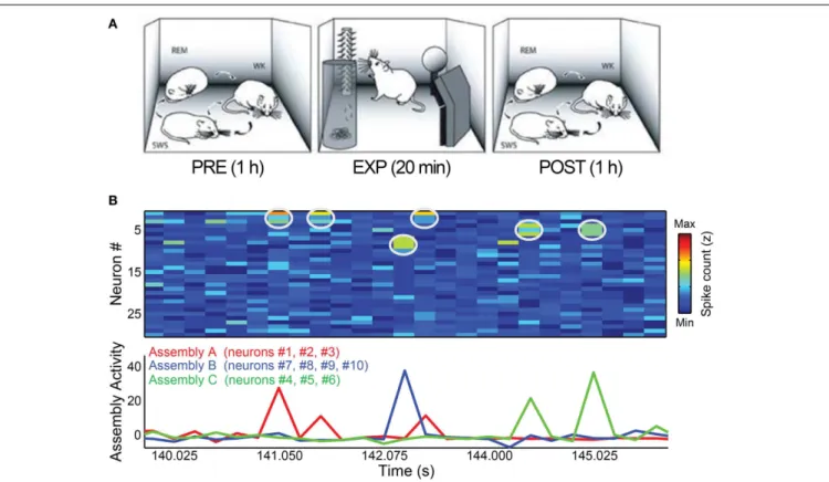
We used data from five Long-Evans adult male rats (300–350 g) recorded before, during and after a novel object exploration paradigm (Ribeiro et al., 2007). The behavioral paradigm began with 1–2 h of recordings as a freely-behaving rat went through the wake-sleep cycle (PRE period). Next, the animal was allowed to explore 4 novel objects placed in the corners of the recording box for 20 min (EXP period). Finally, the objects were removed and the animal was recorded for an additional 1–4 h, freely traversing the wake-sleep cycle (POST period). Video recordings with infrared illumination were used to document behavior. The present study focused on the 1 h PRE and POST periods flanking EXP (Figure 1A).
MULTIELECTRODE ARRAY IMPLANTATION
Briefly, the rats were anesthetized and surgically implanted with multielectrode arrays of tungsten microwires (35µm, 1.0–1.2 MOhm at 1 kHz). A screw implanted on the frontal portion of the skull served as recording ground. The arrays targeted HP, S1, and V1 in the left hemisphere stereotaxic coordinates in mm from Bregma with respect to the antero-posterior (AP), medio-lateral (ML), and dorso-ventral (DV) axes (Paxinos and Watson, 1997): HP (AP:−2.80; ML:+1.5; DV:−3.30); S1 (AP:−3.00; ML: +5.5; DV:−1.40); V1 (AP:−7.30; ML:+4.00; DV:−1.30). DV
measurements were taken with respect to the pial surface. Arrays comprised 16–32 microwires spaced at 250 mm intervals (4×4
arrays for S1 and V1, 2×16 array for HP). In S1 and V1, arrays
were aimed at pyramidal layer V.
ELECTROPHYSIOLOGICAL RECORDINGS AND UNIT SORTING
As described in detail inRibeiro et al. (2007), action potentials (spikes) and local field potentials (LFP) were recorded with multi-electrode arrays placed in the dorsal CA1 region and dentate gyrus of HP, in the barrel field of S1, and in V1. Animals were recorded after a 1-week recovery period following surgery. A 96-channel multineuron acquisition processor (MAP, Plexon Inc, Dallas, TX) was used for digital spike waveform discrimination and storage. Action potentials (spikes) were extracted from the high frequency band data and sorted into units using supervised online spike sorting (SortClient 2002, Plexon Inc.) associated with posterior offline validation (Offline Sorter 2.3, Plexon Inc). LFPs recorded from the same wires were pre-amplified, filtered, and digitized using a Digital Acquisition card (National Instruments, Austin, TX) and a MAP (Plexon Inc). Behaviors were recorded through-out the entire experiment under infrared illumination, by way of two CCD video cameras and a videocassette recorder. Video and neural recordings were synchronized with a millisecond-precision timer (model VTG-55; For-A, Tokyo, Japan). Within each region, the amount of units consisted of 42 HP, 33 S1 and 20 V1 for rat # 1, 59 HP, 23 S1 and 28 V1 for rat # 2, 34 HP, 25 S1 and 23 V1 for rat # 3, 39 HP, 27 S1 and 37 V1 for rat # 4 and 45 HP, 39 S1 and 42 V1 for rat # 5.
SORTING OF BEHAVIORAL STATES
We used LFP data associated with a behavioral state sorting algorithm (Gervasoni et al., 2004) to classify the states with 1 s res-olution. The algorithm is based on a two-dimensional state space defined by two spectral amplitude ratios calculated by divid-ing integrated spectral amplitudes at selected frequency bands. A scatter plot of the two chosen LFP spectral amplitude ratios (state-space) reveals distinct clusters that correspond to the three major wake-sleep states studied here: waking (WK), slow wave sleep (SWS), and rapid eye movement sleep (REM).
ASSEMBLY DETECTION
A cell assembly is a subset of cells that somehow behave as a sin-gle entity. Here we assumed a linear model. More specifically, we defined the activity of a cell assembly as a weighted sum of the activity of individual units. In order to determine the weights of each neuron to each cell assembly we used a recently developed framework (Lopes-dos-Santos et al., 2013), which can be briefly described in four main steps:
(1) The spike train of each neuron was binned into 5 ms windows and z-scored (i.e., variance and mean were set to 1 and 0, respectively). Thus, the population activity was transformed in a matrix in which each element represented the normalized number of spikes of a given neuron in a given time bin. We referred to this matrix asactivity matrix.
FIGURE 1 | Behavioral paradigm and cell assembly detection. (A)Rats were submitted to three periods of experimentation. During PRE and POST periods, animals were kept in a rectangular box freely behaving for 1 h, including complete wake-sleep cycle, sorted here as WK, SWS, and REM. Within EXP period, 4 novel objects were placed in the corners of the box and the animals were free to explore them for 20 min. Figure adapted from
Ribeiro et al. (2007).(B)Toy example of assembly detection and projection of
assembly activity time-series. We simulated 30 independent neurons as Poisson processes with mean 1 spike/bin and created three assemblies (A–C)
by setting 3% of the data (1% for each assembly) as bins with synchronization between the cells of a specific assembly. In this dataset, assembly A comprises neurons # 1, # 2, and # 3; assembly B is formed by neurons # 7, # 8, # 9, and # 10 and neurons # 4, # 5, and # 6 make assembly C. Top panel shows the spike matrix (white circles mark co-activations of assembly neurons). Bottom panel shows the assembly activity time-series, calculated using the ICA-based method described inLopes-dos-Santos et al.
(2013). Note that the assembly activities peak only when their corresponding
neurons co-fire.
(3) The activity matrix was projected into the subspace spanned by the principal components with eigenvalues crossing the statistical threshold and then submitted to Independent Component Analysis (ICA) (Laubach et al., 1999; Hyvärinen and Oja, 2000). Independent components can be understood asassembly patternsthat represent assemblies when the lin-ear model is assumed (Lopes-dos-Santos et al., 2013), i.e., the values attributed to each neuron in a pattern define the weights of the cells in the corresponding assembly.
(4) Individual cell assembly activity was computed by projecting the activity matrix onto its assembly pattern (Lopes-dos-Santos et al., 2013), which can be mathematically defined as:
AAb= Nneurons
i=1
wizib=WTZb,
whereAAb is the assembly activity at time binb,Nneurons is
the total number of neurons,wiis the weight of neuroniin
a specific assembly andzibis the z-scored activity of neuron
iwithin binb. We removed the contribution of single units
firing alone (for instance, if a heavily-weighted neuron acti-vated but others were silent, the assembly activity remained low).
Figure 1B shows an illustrative example of an activity matrix (top panel) along with the assembly activities estimated by the method. For more details, see (Lopes-dos-Santos et al., 2013).
RESULTS
TIME BIN DETERMINATION
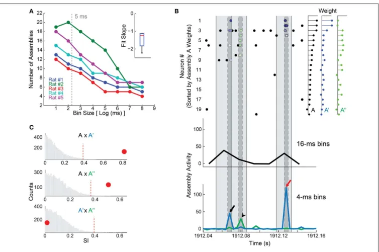
FIGURE 2 | Time bin size influences the detection of cell assemblies. (A)Plot between log2 of bin size in milliseconds and the number of detected assemblies. We assessed bins in a binary scale from 2 to 256 ms. Notice an inverse correlation between log2 of bin size and the number of assemblies; inset shows the distribution of slopes of the linear fits in the main panel. Gray dashed line depicts the 5 ms bin size chosen in our study.(B)(Bottom) 120 ms of assembly activity from animal # 1, showing activity of assembly A (black line), detected in EXP WK with 16 ms bin size, and of assemblies A′
(blue line) and A′′
(green line), detected with a bin size of 4 ms. (Top) Rasterplot of the 20 most relevant neurons that constitute assembly A (80% of the weight), ranked from highest weight to the twentieth highest. Light gray shadow represents 16 ms intervals, dark gray ones represent 4 ms. Blue dots exhibit the spike times of neurons contributing to assembly A′
activity peak (black and red arrows, bottom panel). Green dots mark spikes contributing to assembly A′′activity peak (black arrow head, bottom panel).
Colored dots (spike times) are graded from darker to lighter respective to the
weight of the correspondent neuron in the assembly pattern. Note that neurons participating in assembly A (bin 16 ms) were sorted into assemblies A′
and A′′
(bin 4 ms), which can be active in sequence (black arrow and arrow head) or independently (red arrow).(C)Exploring similarities between assemblies. Panels show the histogram of SI values from 10,000 comparisons made by shuffling the neurons weights within assemblies to build a null hypothesis (bootstrap procedure). Red dashed line shows the threshold for significance atp=0.01. Red circles depict the SI between A
and A′
(0.82, top), A and A′′
(0.51, middle), and A′
and A′′
(0.016, bottom). Note that assembly A is significantly similar to A′and A′′(SI=0
.82 and 0.51,
respectively). The SI between A′and A′′was small (
SI=0.016), indicating
that, in addition to the fact that these assemblies have independent activity, they also have orthogonal membership. A′
and A′′
exhibit strong assembly activations at different time bins (panelB–arrows vs. arrow head). However, when 16 ms time bins were used, the activities of these assemblies were packed in the same time window, causing the merge of A′and A′′into A.
a 16 ms time bin in rat # 1 dataset, and its activity is shown in black (Figure 2B, bottom); while the activities of two assemblies detected using a 4 ms bin size (A′
and A′′
) are depicted in blue and green, respectively (Figure 2B, bottom).
To use a quantitative criterion to compare assembly compo-sition, a Similarity Index (SI) was defined as the absolute value of the inner product between the assembly patterns (unitary vec-tors) of two given assemblies, varying from 0 to 1. Thus, if two assemblies attribute large weights to the same neurons, SI will be large; if assemblies are orthogonal, SI will be zero. We applied a permutation test in order to determine whether SIs were signif-icantly above chance. This test consisted in shuffling the weights
of each pattern across neurons, and then recalculating the SI. We ran 10,000 permutations in order to construct a null hypoth-esis distribution. Two patterns were regarded asrepresentations of the same assembly if their original SI was larger than the 99th percentile of the null hypothesis distribution (i.e.,p=0.01).
Using this process, we found that both A′
and A′′
were signifi-cantly similar to assembly A (Figure 2C). This indicates that units with larger weights in assembly A were split in two independent (SI=0.016) assemblies A′ and A′′ comprising partially
sequences (Figure 2B), we chose the 5 ms bin as a compromise between a high temporal resolution and the need to avoid small bin sizes close to the neuronal refractory period.
SEARCHING FOR ASSEMBLIES IN DIFFERENT EXPERIMENTAL PERIODS
After defining bin size, we focused on the assessment of the dif-ferences among assemblies detected using spike matrices from different experimental periods (PRE, EXP and POST). Our goal was to investigate whether the exposure to novel objects changes the assembly repertoire. At first we ignored sleep states and extracted assembly patterns from entire PRE, EXP and POST-WK periods (each one independently). Next, we used the SI to compare all assemblies between experimental periods.
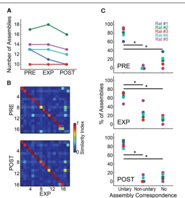
We found little variation in the numbers of assemblies across different experimental periods (Figure 3A). Most animals showed a maintenance or minor decrease in the number of assemblies from PRE to EXP, except for rat # 2, which showed an increase of one assembly. From EXP to POST, the number of assemblies detected also dropped slightly, except for rat # 3, which showed a stable number of 10 assemblies per period. Rat # 1 showed the highest variance in the number of assemblies detected across peri-ods, ranging from 13 in PRE to 10 in POST.Figure 3Billustrates the substantial similarity between assemblies detected in differ-ent experimdiffer-ental periods for rat # 2, which overall showed the largest number of assemblies. To assess assembly conservation across experimental periods, we then categorized the assemblies within each experimental period as showing unitary correspon-dence, non-unitary corresponcorrespon-dence, or no correspondence. An assembly was considered to show unitary correspondence when it was significantly similar to only one assembly in each of its flanking experimental period(s) with p<0.0001; non-unitary
correspondence defined assemblies which showed more than one correspondence or, in the case of EXP, those with correspon-dence to one assembly from a flanking period but not with the other (e.g., correspondence with PRE but not with POST); the no-correspondence category comprised assemblies showing no significant correspondences. Group results across different exper-imental periods (Figure 3C) show that the number of assemblies exhibiting unitary correspondence was significantly higher than those showing non-unitary correspondence or no correspon-dence, including EXP which is flanked by two neighbor periods (Wilcoxon ranksum test,p<0.05, Bonferroni corrected).
A comparison across experimental periods reveals that the percentage in PRE of assemblies with no correspondence was slightly elevated, while non-unitary correspondence was very minor. During EXP the percentage of non-unitary dences increased, while the percentage of unitary correspon-dences and no-corresponcorrespon-dences decreased. This could represent the fact that EXP is flanked by two neighbor periods, while PRE and POST are flanked by only one. Another possible explanation is that the exposure to novel objects could have changed some assembly activation patterns, increasing their co-activations (see
Figure 6B), and causing separate assemblies to be detected as one. This may decrease the SI, leading to non-significance between similar assemblies, and/or to significant similarity of one assem-bly with two or more assemblies from flanking periods, compris-ing significant but lower SIs. The POST period showed the highest
FIGURE 3 | Cell assemblies are highly conserved across experimental periods. (A)Number of assemblies detected using spike matrices from the different experimental periods.(B)SI values among assembly patterns of rat #2 across experimental periods. Assembly patterns were detected using a 5 ms bin size. Assembly labels were sorted to let highest values in the main diagonal.(C)For each experimental period, the panels show the percentages of assemblies within each of the categories defined by the number of significant correspondences between the assemblies of a given experimental period and the assemblies from flanking periods (from top to bottom, PRE, EXP and POST). Two assembly patterns were deemed correspondent if their SI was above a threshold set by a bootstrap procedure (p=0.0001). The categories were defined as unitary
correspondence, non-unitary correspondence and no correspondence, representing the percentage of assemblies within rats that showed, respectively, a single correspondence between flanking periods, two or more flanking correspondences, or no correspondence whatsoever. Note that the percentage of assemblies within the unitary correspondence category was considered significantly higher than the other categories for all experimental periods (Wilcoxon ranksum test,∗
p<0.05, Bonferroni
corrected).
over the entire recording, throughout the wake-sleep cycle. Using this approach, we detected 11, 18, 10, 13 and 13 assemblies for rats # 1 to # 5, respectively.
DETECTING ASSEMBLY ACTIVATIONS
In order to improve the time resolution for the analysis of assem-bly activation sequences, we first re-binned the spike trains from each unit using 1 ms bins, and convolved the data with a Gaussian kernel (maximum=1, 80% of the AUC within 5 ms windows).
Then we projected the activity of all assemblies, and defined a threshold (for each assembly) as the 99th percentile of the distri-bution of activity values across time bins (Figure 4A, red lines).
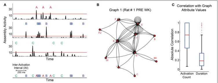
Figure 4Ashows the activity of three exemplary assemblies (A, B, and C) from rat # 1, which above-threshold peaks are depicted by red, blue and green letters (assembly activations), respec-tively. Subsequent assembly activation was only considered after a “refractory” period of 3 ms elapsed.
CALCULATION OF ASSEMBLY GRAPH ATTRIBUTES
We constructed the assembly activation sequence by labeling and concatenating assembly activations from different assemblies (Figure 4A, bottom). Graphs were built from this sequence, so that each assembly corresponded to a node, each edge corre-sponded to the temporal sequence of consecutive node activa-tions, and the time intervals between two assembly activations were considered inter-activation intervals (IAI) (Figure 4A, bot-tom). The coactivation of two or more assemblies within the same time bin was represented as an additional node in the graph, whose label comprised the labels of the assemblies activated at the same time. For instance, if assemblies F and J displayed
synchronous activation, a fourth node FJ was added to the graph, always in the alphabetical order (Figure 4B).
Two parameters shaped the graphs: maximum IAI and num-ber of activations per graph (activation count). The maximum IAI parameter defined the threshold IAI within each graph, i.e., every time interval between assembly activations within a graph should be less than or equal to this maximum IAI. Seven different maximum IAI values ranging from 10 to 1000 ms were explored.
An initial assessment of the data varying only the maxi-mum IAI criterion showed that, in general, the assembly graph attributes were proportional to the activation count in a graph (Figure 4C, median of absolute Pearson correlation indexes dis-tribution=0.74), while the duration (the interval between the
first and last assembly activation within a graph) was not corre-lated to assembly graph attributes (Figure 4C, median of absolute Pearson correlation indexes distribution=0.18).
A fixed number of assembly activations per graph was used to control for this variability in the graph attributes. Since the minimum activation count necessary to maximize the density of a graph (Table 1) is the square of the number of nodes –Number of Assemblies2, we evaluated seven values of activa-tion count as percentages of Number of Assemblies2 (10, 20, 50, 100, 120, 150 and 200%). The custom-made java software Speechgraphs(Mota et al., 2012; http://neuro.ufrn.br/softwares/
speechgraphs) was used to calculate 13 assembly graph attributes (Table 1).
CHANGES IN POPULATION RATE DO NOT EXPLAIN THE ACTIVITY OF
INDIVIDUAL ASSEMBLIES
The algorithm to algebraically define assembly activity was the squared linear combination of the firing rate of the units in a
FIGURE 4 | Determination of sequences of cell assembly activations. (A)1.5 s interval showing activity of 3 assemblies (A–C) of rat # 1 (3 top panels). Thresholds are the 99th percentiles of the activity values for each assembly. Threshold-crossing peaks are considered assembly activations. Assembly activation sequence is defined as the series of activation across different assemblies within subjects; and the time interval between two subsequent activations is called inter-activation interval (IAI) (bottom panel).
(B)Exemplary graph generated with assembly activations from the first WK
episode of rat # 1 during PRE.(C)Distribution of absolute Pearson correlation values between graph attributes and two other variables: activation count and graph duration. Graphs were generated using assembly activation sequences from behavioral states’ episodes. Panel shows distribution of data from all episodes. Note that activation count was generally correlated with graph attribute values in our dataset (median=0.74, 74% of correlations were significant withp<0.05), while the graphs duration were not (median=
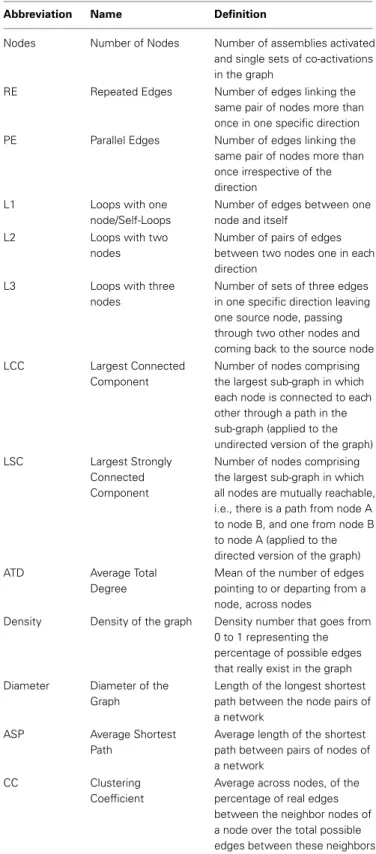
Table 1 | Graph attributes.
Abbreviation Name Definition
Nodes Number of Nodes Number of assemblies activated
and single sets of co-activations in the graph
RE Repeated Edges Number of edges linking the
same pair of nodes more than once in one specific direction
PE Parallel Edges Number of edges linking the
same pair of nodes more than once irrespective of the direction
L1 Loops with one
node/Self-Loops
Number of edges between one node and itself
L2 Loops with two
nodes
Number of pairs of edges between two nodes one in each direction
L3 Loops with three
nodes
Number of sets of three edges in one specific direction leaving one source node, passing through two other nodes and coming back to the source node
LCC Largest Connected
Component
Number of nodes comprising the largest sub-graph in which each node is connected to each other through a path in the sub-graph (applied to the undirected version of the graph)
LSC Largest Strongly
Connected Component
Number of nodes comprising the largest sub-graph in which all nodes are mutually reachable, i.e., there is a path from node A to node B, and one from node B to node A (applied to the directed version of the graph)
ATD Average Total
Degree
Mean of the number of edges pointing to or departing from a node, across nodes
Density Density of the graph Density number that goes from 0 to 1 representing the percentage of possible edges that really exist in the graph
Diameter Diameter of the
Graph
Length of the longest shortest path between the node pairs of a network
ASP Average Shortest
Path
Average length of the shortest path between pairs of nodes of a network
CC Clustering
Coefficient
Average across nodes, of the percentage of real edges between the neighbor nodes of a node over the total possible edges between these neighbors
given time bin (Lopes-dos-Santos et al., 2011, 2013). Hence, while assembly activity is dependent on population firing rate, it is not fully determined by it, because its projection also depends on the weight of each unit on that specific assembly.
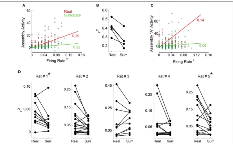
A plethora of studies have shown that firing rate changes con-vey behavioral information (Adrian and Zotterman, 1926; Hubel and Wiesel, 1959; O’Keefe and Dostrovsky, 1971; Moritz et al., 2008); thus, it was first important to show that assembly activ-ity is not just an epiphenomenon of population rate. To address this issue, we plotted the squared mean population rate against the mean of all assemblies’ activity within each bin along the whole experiment for each rat (Figure 5Afor rat # 1, dark red dots). TheR2 of the linear fit between these two variables was low for all animals (Figure 5B), indicating that they display a weak correlation. We then plotted the same squared mean of the population rate against the mean assembly activity projected using spike matrices with surrogated rates within each single bin (Figure 5A, dark green dots). This allowed us to vary one of the variables that define assembly activity (weights of each unit within each assembly), while keeping the other unchanged (population rate). This approach showed linear fits with even lowerR2 val-ues (Figure 5A, light green line for rat # 1 and Figure 5B for all rats).
Next we investigated activity time-series of individual assem-blies (Figure 5C, exemplary assembly from rat # 1).Figure 5D
showsR2 values for the linear fits from all individual assem-blies as in Figure 5C, for all animals (real data—left; surro-gated data—right). All values are very low, and become even lower when we use the surrogated dataset, including a sta-tistically significant difference in R2 values between real and surrogated datasets, for rats # 1 and # 5. (Figure 5D, aster-isk, Wilcoxon signed-rank paired test, p<0.05). Altogether,
these results indicate that the activity of individual assem-blies is not reducible to fluctuations of the population firing rate.
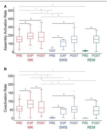
ASSEMBLY ACTIVATION RATE AND COACTIVATIONS
We analyzed assembly activation time-series (Figure 6A, exem-plary plot from rat # 5) from all behavioral states (WK, SWS and REM) and experimental periods (PRE, EXP and POST). Considering all rats, we found that the assembly activation rate during WK was significantly higher in almost all the paired com-parisons (18 out of 21) of experimental periods between behav-ioral states (gray lines with asterisk,p<0.05, Wilcoxon ranksum
FIGURE 5 | The activity of individual assemblies is not reducible to rate fluctuations. (A,C)show exemplary panels from rat # 1 and(B,D)show group data.(A)Squared mean of the population rate and the mean of all assemblies’ activity within each 1 ms bin (dark red dots). In order to scramble associative behavior and keep the firing rate fixed, we also plotted the mean population rate against the mean assemblies’ activity projected using the spike matrix with neurons’ labels surrogated within each time bin (dark green dots). Light red and green lines depict the least square linear fit for each color coded subset of points along with the correspondent coefficients of determination (R2).(B)Coefficient of determination distribution for all rats.
For all animals, data surrogation impaired the correlation between firing rate and assembly activity.(C)The same color code as in(A), but plotting the mean population rate against the activity of a single exemplary assembly from rat # 1.(D)Shown are distributions of all ratsR2values for the linear fits
from the correlation between mean population rate and individual
assemblies’ activity (left) and mean population rate and individual assemblies’ activity estimated from surrogated spike matrices (right). Note that both distributions exhibit very lowR2values and that there is a decreasing trend
from real to surrogated data, with significant difference for rats # 1 and # 5 (∗p
<0.05, Wilcoxon signed-rank paired test).
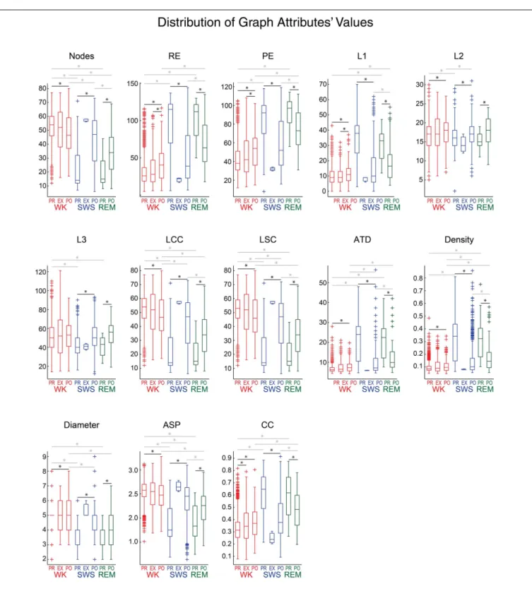
GRAPH ANALYSIS
We found that graph attributes varied significantly across behavioral states and experimental periods (Figure 7). We tested therefore whether a Naïve Bayes classifier could extract, from the assembly graph attributes, information enough to sort behav-ioral states and experimental periods (John and Langley, 1995). We used the java softwareWeka (http://www.cs.waikato.ac.nz/
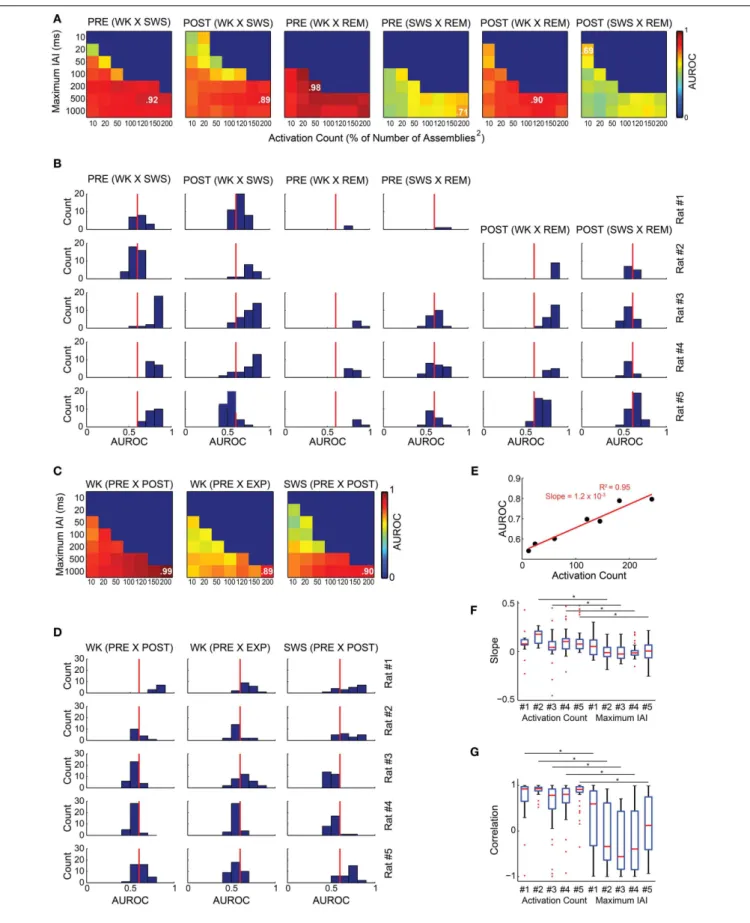
ml/weka/) to perform the classifications and estimated their qual-ity by the area under the receiver operating characteristic curve (AUROC).Figures 8A,Bshow that it was possible to sort behav-ioral states with very high quality of classification, particularly when WK and REM were compared (maximum AUROCs ranging from 0.78 to 0.98). WK and SWS could also be distinguished, at a somewhat lower level (maximum AUROCs ranging from 0.69 to 0.96). The poorest quality of classification was obtained by sort-ing SWS from REM (maximum AUROCs rangsort-ing from 0.64 to 0.78).
The classification quality across experimental periods was not as good as across behavioral states (median across rats 0.57
vs. 0.69, Wilcoxon ranksum test, p<0.01), except for rat # 1. Figures 8C,D show that the maximum AUROC values for the comparisons between experimental periods ranged from 0.55 to 0.99, with distribution of all values yielding 0.52 and 0.67 as the first and third quartiles, compared to 0.58 and 0.84, as quartiles for the comparisons between behavioral states. We found a strong positive correlation between the AUROC of graph attributes and activation count for all the comparisons made (e.g., rats # 4 and # 1 inFigures 8A,C). One example of this correlation is shown on a plot of the AUROC values from the classification between PRE WK and PRE SWS vs. the activation count of the graphs of rat # 1, considering only values obtained using the 1000 ms maximum IAI (Figure 8E). The figure shows a positive correla-tion associated with an extremely strong linear fit (R2=0.95)
and a 1.2×10⁻³ slope, in association with major variation in
FIGURE 6 | Descriptive statistics.Panels show the distribution of assembly activation rate(A)and co-activation rate(B)(events per second) during different behavioral states and experimental periods for rat # 5. Behavioral states boxplots are color coded as red, blue, and green for WK, SWS and REM, respectively. Experimental periods (PRE, EXP and POST) are placed together and in chronological sequence within each behavioral state. Black lines with asterisks reflect significance between two different experimental periods within a given behavioral state. Gray lines with asterisks reflect significance between two different behavioral states within a given experimental period (p<0.05, bootstrap corrected for multiple
comparisons).
the AUROCs vs. the maximum IAIs considering a constant acti-vation count for the panels from all rats. Note that actiacti-vation count accounts for AUROC variability significantly more than the maximum IAI, except for rat # 1 (Figure 8F), according to a pos-itive correlation (Figure 8G). It is important to note that there was no AUROC above 0.68 when we used maximum IAIs below 20 ms. Maximum AUROCs were obtained using each of the seven different activation counts explored.
DISCUSSION
Our results show that assembly graphs comprising synchronized neuronal units recorded from the hippocampus and primary sen-sory cortices can be used to sort behavioral states (maximum AUROC values ranging from 0.64 to 0.98) and experimental peri-ods (maximum AUROC values ranging from 0.55 to 0.99) before, during and after novel object exploration. This sorting is based on several attributes that reflect the structural properties of assembly graphs. At this point we do not know whether these attributes are informative due to a causal relationship with behavior, or
as an epiphenomenon of some other underlying cause. In all, our investigation corroborates the notion that phase sequences, understood as specific patterns of assembly activations, reflect the different regimes of neural processing as animals traverse the wake-sleep cycle and acquire novel information about the environment.
Such interpretation of the results cannot be furthered with-out addressing the problem of the arbitrary definition of time scale for synchronous firing. As shown inFigure 2A, the number of assemblies detected decreases with bin size. We showed evi-dence that this may be due to the tight temporal association of assemblies detected using smaller bin sizes, which are detected as a single assembly when larger bin sizes are used. Our choice of bin size=5 ms for the generation of assembly graphs, well within the
potentiation window of spike time dependent plasticity (STDP) (Bi and Poo, 1998), represents a compromise between the num-ber of assemblies detected and the need to avoid extremely low bin sizes near the neuronal refractory period.
Our results show that the repertoire of assemblies is almost unchanged across experimental periods, which suggests that novel experience does not create new assemblies in the hippocam-pus and primary sensory neocortex of the normal adult rat. Our finding is compatible with Hebb’s hypothesis that assemblies correspond to the primitive building blocks of representations, being slowly formed across development but nearly unchanged in adulthood. The experience-dependent changes in the structure of assembly graphs, revealed by the use of a classifier, also cor-roborates the complementary Hebbian hypothesis that relevant information about concepts, percepts and behavior in general is coded at the level of multiple assembly activations, the so called phase sequences (Hebb, 1949).
We also showed that the activity of single assemblies cannot be reduced to the changes in firing rate. Changes in neuronal firing rates constitute well-known indexes of behavior (Adrian and Zotterman, 1926; Hubel and Wiesel, 1959; O’Keefe and Dostrovsky, 1971; Moritz et al., 2008). If phase sequences are indeed important to generate new neural representations, they should carry more specific information than firing rates. Since assemblies are subsets of neurons that function transiently as closed systems, the neurons related to a given perception or behavior should have their rates affected synchronously, so as to be detected as assemblies. The calculation of assemblies and the projection of their activity is a way to reduce the dimension-ality of a population of neuronal units onto neuronal subsets which are likely related to behavior. Investigation of whether phase sequences carry more information than firing rates is ongoing.
FIGURE 7 | Assembly graph attributes vary significantly across behavioral states and experimental periods.Panels show the
distribution of graph attributes’ values from rat # 5, using 1 s maximum IAI and 169 activations/graph, for different behavioral states and experimental periods. As inFigure 6, behavioral states boxplots are color coded as red, blue, and green for WK, SWS and REM, respectively. Experimental periods (PRE, EXP and POST) are placed together and in chronological sequence within each behavioral state. Black lines with asterisks reflect significance between two different experimental periods within episodes of a given behavioral state (p<0.05, Wilcoxon ranksum test, Bonferroni corrected).
Gray lines with asterisks reflect significance between two different
behavioral states within a given experimental period. Note that nearly all the attributes sorted WK from SWS, during PRE or POST (except for L1 during PRE and L3 during POST). WK was significantly different from REM during PRE (12 attributes) and POST (11 attributes), SWS was significantly different from REM during POST (10 attributes), but no attribute could sort SWS and REM during PRE. Only one attribute was capable of sorting PRE from EXP within WK. When comparing PRE×POST within WK, 12
FIGURE 8 | Assembly graph attributes allow for the automatic classification of experimental periods and behavioral states. (A,C)The rows of each panel represent the graphs maximum IAI (within the graph, every IAI is less than or equal to the maximum IAI value), while the columns
correspond to the number of activations within the graphs defined as percentages of the squared number of assemblies. Color codes vary from 0 to 1 and represent the median AUROC of 50 classifications made for 20
FIGURE 8 | Continued
random graphs from each of the experimental periods compared using a Naïve Bayes classifier; e.g., 20 graphs from PRE WK compared with 20 graphs from EXP WK. In some cases of the parameter screening, we could not obtain the minimum 20 graphs necessary for the classification. For instance, it was impossible to generate one single graph comprising 200 activations (200% of
Number of Assemblies2for rat # 3) within the 10 ms maximum IAI. These conditions were coded blue to indicate no classification. The maximum AUROC value of each panel is indicated.(A,B)Sorting of behavioral states.(A)Panels show the classification quality across different maximum IAI and activation count values for rat # 4.(B)Histograms of AUROC values as in panel(A)for all rats. Red line depicts the 0.6 AUROC value, which sets the lower bound for a good classification quality. WK and REM were well sorted by graph attributes, with maximum AUROC values ranging from 0.68 to 0.98 for all rats within both PRE and POST periods. The sorting of SWS and REM was substantially less accurate, with maximum AUROC=0.78 during POST in rat # 5. The sorting between WK and REM was very good for all rats during PRE, (maximum AUROCs from 0.78 to 0.98).(C,D)Sorting of experimental periods.(C)Panels show the classification quality for rat # 1 across different maximum IAI and activation count values.(D)Histograms of AUROC values from the panels as in panel(C)for all rats. All the comparisons yielded maximum AUROCs ranging from 0.55 to 0.99.(E)Correlation between AUROC and activation count using a
1000 ms maximum IAI from rat # 1 graphs comparing PRE WK and PRE SWS. The slope of the linear fit indicates that each single activation added to a graph, adds 0.0012 to the AUROC, with activation counts varying from 12 to 242 (AUROCs vary from 0.54 to 0.80).(F)Distribution of slopes of the linear fits between activation count and AUROC with fixed maximum IAI value (e.g., panel
E); and between maximum IAIs and AUROC with fixed activation count. We used the AUROCs from all the comparisons and conditions (maximum IAI and activation counts) for all animals and considered only fits with three or more data points. The analysis shows that the maximum IAI contribution to the AUROC is around zero (mean across rats=0.0024) and even negative, while the contribution of the activation count is divergent, with a clear majority of positive contributions (mean across rats=0.097), yielding a significant
difference between these two variables, except for rat # 1(G)Distribution of Pearson correlations indexes for the comparisons in panel(F). Note that activation count shows strong positive correlation with AUROCs (medians=
0.92, 0.93, 0.78, 0.80, and 0.91 for rats # 1 to # 5, respectively; 53% of the values withp<0.05), while maximum IAIs are scattered, with values spanning
the entire scale, and medians closer to zero or even negative for all rats (0.59,
−0.33,−0.56,−0.39, and 0.12 for rats # 1 to # 5, respectively; 8% of the values withp<0.05). Asterisks indicate significant differences between activation
count and maximum IAI distributions of correlation values within the same animal.
It is important to point out that in the present study we assumed that the activity of a cell assembly could be described as a linear combination of the activity of individual neurons. While this simplification of the assembly model allows for the analy-sis of large neuronal populations, it also presents some potential caveats (Lopes-dos-Santos et al., 2013). In particular, strong non-linear correlations between neurons may lead to spurious results, since both the determination of the number of assemblies and the extraction of assembly patterns are based on the linear model. Nevertheless, because this representation of assemblies is intuitive and straightforward, it is possible to verify the outcomes of the analysis; for instance, visual inspection of the raw data confirms that co-activations of assembly members correspond to peaks in assembly activity (seeFigure 2B, also see examples employ-ing similar linear methods in (Nicolelis et al., 1995; Peyrache et al., 2009, 2010; Benchenane et al., 2010; Lopes-dos-Santos et al., 2011, 2013). In principle, a non-linear method should be more robust and realistic, but we are not aware of any non-linear method capable of extracting assembly composition from the ongoing activity of neuronal populations with dozens of neu-rons. An ideal method should also incorporate information on the physiology of specific cell types and neural circuits. Taken together, our results show that, despite any possible non-linear correlations that may exist among neurons, the linear ones carry relevant information that support a role for phase sequences in behavior and cognition. Future research shall include non-linear modeling and also consider a neural coding approach, in order to fully characterize the repertoires of phase sequences, and elu-cidate the role of specific graph attributes in the representation of contextual cues, sensory stimuli and motor behavior.
AUTHOR CONTRIBUTIONS
Sidarta Ribeiro collected the data; Daniel G. Almeida-Filho, Nivaldo A. P. Vasconcelos, Vitor Lopes-dos-Santos, and Sidarta Ribeiro analyzed the data; Daniel G. Almeida-Filho prepared the figures; Daniel G. Almeida-Filho, Sidarta Ribeiro, Nivaldo A. P.
Vasconcelos, Vitor Lopes-dos-Santos, Adriano B. L.Tort, and José G. V. Miranda wrote the manuscript.
ACKNOWLEDGMENTS
Support was obtained from the Pew Latin American Fellows Program in the Biomedical Sciences, Financiadora de Estudos e Projetos (FINEP)—Grant 01.06.1092.00, Ministério da Ciência e Tecnologia e Inovação (MCTI), CNPq Universal 481351/2011-6, PQ 306604/2012-4, Coordenação de Aperfeiçoamento de Pessoal de Nível Superior (CAPES), FAPERN/CNPq Pronem 003/2011, Capes SticAmSud, FAPESP Center for Neuromathematics (grant #2013/ 07699-0, São Paulo Research Foundation), and NIMBIOS working group “Multi-scale analysis of cortical networks.” We thank N. B. Mota, P. Petrovitch, and R. Furtado for help with the SpeechGraphs software, A. Karla for administrative help, and D. Koshiyama for library support.
REFERENCES
Adrian, E. D., and Zotterman, Y. (1926). The impulses produced by sensory nerve-endings Part II.The response of a Single End-Organ.J. Physiol.61, 151–171. Benchenane, K., Peyrache, A., Khamassi, M., Tierney, P. L., Gioanni, Y., Battaglia, F.
P., et al. (2010). Coherent theta oscillations and reorganization of spike timing in
the hippocampal-prefrontal network upon learning.Neuron66, 921–936. doi:
10.1016/j.neuron.2010.05.013
Berger, D., Borgelt, C., Louis, S., Morrison, A., and Grün, S. (2010). Efficient iden-tification of assembly neurons within massively parallel spike trains.Comput. Intell. Neurosci.2010, 1. doi: 10.1155/2010/439648
Bi, G.-Q., and Poo, M.-M. (1998). Synaptic modifications in cultured hippocampal neurons: dependence on spike timing, synaptic strength, and postsynaptic cell type.J. Neurosci.18, 10464–10472.
Bliss, T. V., and Collingridge, G. L. (1993). A synaptic model of memory: long-term
potentiation in the hippocampus.Nature361, 31–39. doi: 10.1038/361031a0
Buzsáki, G. (2004). Large-scale recording of neuronal ensembles.Nat. Neurosci.7, 446–451. doi: 10.1038/nn1233
Canolty, R. T., Ganguly, K., Kennerley, S. W., Cadieu, C. F., Koepsell, K., Wallis, J. D., et al. (2010). Oscillatory phase coupling coordinates anatomically dispersed functional cell assemblies.Proc. Natl. Acad. Sci.U.S.A.107, 17356–17361. doi: 10.1073/pnas.1008306107
two-year-old rat hippocampusin vitro.Neurobiol. Aging 12, 517–522. doi: 10.1016/0197-4580(91)90082-U
Deisseroth, K., Bito, H., Schulman, H., and Tsien, R. (1995). Synaptic plastic-ity: a molecular mechanism for metaplasticity.Curr. Biol.5, 1334–1338. doi: 10.1016/S0960-9822(95)00262-4
Denker, M., Riehle, A., Diesmann, M., and Grün, S. (2010). Estimating the con-tribution of assembly activity to cortical dynamics from spike and population
measures.J. Comput. Neurosci.29, 599–613. doi: 10.1007/s10827-010-0241-8
Dragoi, G., and Tonegawa, S. (2010). Preplay of future place cell sequences by
hip-pocampal cellular assemblies.Nature469, 397–401. doi: 10.1038/nature09633
Gervasoni, D., Lin, S. C., Ribeiro, S., Soares, E. S., Pantoja, J., and Nicolelis, M. A. L. (2004). Global forebrain dynamics predict rat behavioral states and their
tran-sitions.J. Neurosci.24, 11137–11147. doi: 10.1523/JNEUROSCI.3524-04.2004
Harris, K. D. (2005). Neural signatures of cell assembly organization.Nat. Rev. Neurosci.6, 399–407. doi: 10.1038/nrn1669
Harris, K. D., Csicsvari, J., Hirase, H., Dragoi, G., and Buzsáki, G. (2003). Organization of cell assemblies in the hippocampus.Nature424, 552–556. doi: 10.1038/nature01834
Hebb, D. (1949).The Organization of Behavior. New York, NY: Wiley.
Hobson, J. A., and McCarley, R. W. (1971). Cortical unit activity in sleep and waking.Electroencephalogr. Clin. Neurophysiol.30, 97–112. doi: 10.1016/0013-4694(71)90271-9
Hubel, D. H., and Wiesel, T. N. (1959). Receptive fields of single neurones in the cat’s striate cortex.J. Physiol.148, 574–591.
Hyvärinen, A., and Oja, E. (2000). Independent component analysis:
algo-rithms and applications. Neural Netw. 13, 411–430. doi:
10.1016/S0893-6080(00)00026-5
Ikegaya, Y., Aaron, G., Cossart, R., Aronov, D., Lampl, I., Ferster, D., et al. (2004). Synfire chains and cortical songs: temporal modules of cortical activity.Science
304, 559–564. doi: 10.1126/science.1093173
Ji, D., and Wilson, M. A. (2006). Coordinated memory replay in the visual
cortex and hippocampus during sleep. Nat. Neurosci. 10, 100–107. doi:
10.1038/nn1825
John, G. H., and Langley, P. (1995). “Estimating continuous distributions in Bayesian classifiers,” inProceedings of the Eleventh conference on Uncertainty in artificial intelligence (San Francisco, CA: Morgan Kaufmann Publishers Inc.), 338–345.
Klintsova, A. Y., and Greenough, W. T. (1999). Synaptic plasticity in cortical
sys-tems.Curr. Opin. Neurobiol.9, 203–208. doi: 10.1016/S0959-4388(99)80028-2
Kraus, B. J., Robinson Ii, R. J., White, J. A., Eichenbaum, H., and Hasselmo, M.
E. (2013). Hippocampal time cells: time versus path integration.Neuron78,
1090–1101. doi: 10.1016/j.neuron.2013.04.015
Laubach, M., Shuler, M., and Nicolelis, M. A. (1999). Independent component analyses for quantifying neuronal ensemble interactions.J. Neurosci. Methods
94, 141–154. doi: 10.1016/S0165-0270(99)00131-4
Lee, A. K., and Wilson, M. A. (2002). Memory of sequential experience in the
hip-pocampus during slow wave sleep.Neuron36, 1183–1194. doi:
10.1016/S0896-6273(02)01096-6
Liu, X., Ramirez, S., Pang, P. T., Puryear, C. B., Govindarajan, A., Deisseroth, K., et al. (2012). Optogenetic stimulation of a hippocampal engram activates fear
memory recall.Nature484, 381–385. doi: 10.1038/nature11028
Lopes-dos-Santos, V., Conde-Ocazionez, S., Nicolelis, M. A. L., Ribeiro, S. T., and Tort, A. B. L. (2011). Neuronal assembly detection and cell
member-ship specification by principal component analysis.PLoS ONE6:e20996. doi:
10.1371/journal.pone.0020996
Lopes-dos-Santos, V., Ribeiro, S., and Tort, A. B. (2013). Detecting cell
assem-blies in large neuronal populations.J. Neurosci. Methods220, 149–166. doi:
10.1016/j.jneumeth.2013.04.010
Macdonald, C. J., Lepage, K. Q., Eden, U. T., and Eichenbaum, H. (2011). Hippocampal time cells bridge the gap in memory for discontiguous events.
Neuron71, 737–749. doi: 10.1016/j.neuron.2011.07.012
Marˇcenko, V. A., and Pastur, L. A. (1967). Distribution of
eigenval-ues for some sets of random matrices. Mat. Sb. 1, 457–483. doi:
10.1070/SM1967v001n04ABEH001994
Moritz, C. T., Perlmutter, S. I., and Fetz, E. E. (2008). Direct control of paralysed
muscles by cortical neurons.Nature456, 639–642. doi: 10.1038/nature07418
Mota, N. B., Vasconcelos, N. A. P., Lemos, N., Pieretti, A. C., Kinouchi, O., Cecchi, G. A., et al. (2012). Speech graphs provide a quantitative measure of thought
disorder in psychosis.PLoS ONE7:e34928. doi: 10.1371/journal.pone.0034928
Nicolelis, M. A., Baccala, L. A., Lin, R., and Chapin, J. K. (1995). Sensorimotor encoding by synchronous neural ensemble activity at multiple levels of
the somatosensory system. Science 268, 1353–1358. doi: 10.1126/science.
7761855
Nicolelis, M. A. L., Dimitrov, D., Carmena, J. M., Crist, R., Lehew, G., Kralik, J. D., et al. (2003). Chronic, multisite, multielectrode recordings
in macaque monkeys.Proc. Natl. Acad. Sci.U.S.A. 100, 11041–11046. doi:
10.1073/pnas.1934665100
Noda, H., Manohar, S., and Adey, W. R. (1969). Spontaneous activity of cat
hip-pocampal neurons in sleep and wakefulness.Exp. Neurol.24, 217–231. doi:
10.1016/0014-4886(69)90016-8
O’Keefe, J., and Dostrovsky, J. (1971). The hippocampus as a spatial map. Preliminary evidence from unit activity in the freely-moving rat.Brain Res.34, 171–175. doi: 10.1016/0006-8993(71)90358-1
Pastalkova, E., Itskov, V., Amarasingham, A., and Buzsáki, G. (2008). Internally gen-erated cell assembly sequences in the rat hippocampus.Science321, 1322–1327. doi: 10.1126/science.1159775
Paxinos, G., and Watson, C. (1997).The Rat Brain in Stereotaxic Coordinates. San Diego, CA: Academic Press.
Peyrache, A., Benchenane, K., Khamassi, M., Wiener, S. I., and Battaglia, F. P. (2010). Principal component analysis of ensemble recordings reveals cell
assemblies at high temporal resolution.J. Comp. Neurosci.29, 309–325. doi:
10.1007/s10827-009-0154-6
Peyrache, A., Khamassi, M., Benchenane, K., Wiener, S. I., and Battaglia, F. P. (2009). Replay of rule-learning related neural patterns in the prefrontal cortex during sleep.Nat. Neurosci.12, 919–926. doi: 10.1038/nn.2337
Pfeiffer, B. E., and Foster, D. J. (2013). Hippocampal place-cell sequences depict future paths to remembered goals.Nature497, 74–79. doi: 10.1038/nature12112 Ramirez, S., Liu, X., Lin, P. A., Suh, J., Pignatelli, M., Redondo, R. L., et al. (2013). Creating a false memory in the hippocampus.Science341, 387–391. doi: 10.1126/science.1239073
Ribeiro, S., Shi, X., Engelhard, M., Zhou, Y., Zhang, H., Gervasoni, D., et al. (2007). Novel experience induces persistent sleep-dependent
plastic-ity in the cortex but not in the hippocampus. Front. Neurosci.1:43. doi:
10.3389/neuro.01.1.1.003.2007
Robbe, D., Montgomery, S. M., Thome, A., Rueda-Orozco, P. E., Mcnaughton, B. L., and Buzsaki, G. (2006). Cannabinoids reveal importance of spike
tim-ing coordination in hippocampal function.Nat. Neurosci.9, 1526–1533. doi:
10.1038/nn1801
Schrader, S., Grün, S., Diesmann, M., and Gerstein, G. L. (2008). Detecting synfire chain activity using massively parallel spike train recording.J. Neurophysiol.100, 2165–2176. doi: 10.1152/jn.01245.2007
Stopfer, M., Bhagavan, S., Smith, B. H., and Laurent, G. (1997). Impaired odour
dis-crimination on desynchronization of odour-encoding neural assemblies.Nature
390, 70–74. doi: 10.1038/36335
Vanderwolf, C. (1969). Hippocampal electrical activity and voluntary movement in the rat.Electroencephalogr. Clin. Neurophysiol.26, 407–418. doi: 10.1016/0013-4694(69)90092-3
Wilson, M. A., and McNaughton, B. L. (1994). Reactivation of hippocampal
ensemble memories during sleep. Science 265, 676–679. doi:
10.1126/sci-ence.8036517
Conflict of Interest Statement:The authors declare that the research was con-ducted in the absence of any commercial or financial relationships that could be construed as a potential conflict of interest.
Received: 20 December 2013; accepted: 19 March 2014; published online: 08 April 2014.
Citation: Almeida-Filho DG, Lopes-dos-Santos V, Vasconcelos NAP, Miranda JGV, Tort ABL and Ribeiro S (2014) An investigation of Hebbian phase sequences as assembly graphs. Front. Neural Circuits8:34. doi: 10.3389/fncir.2014.00034 This article was submitted to the journal Frontiers in Neural Circuits.