!"
# $ % & ' ( ) '
* +, - ./0 1 & 2 ' / +, & , . '
3 4 2 11 / ' 5 6 7 / '
2 +, 8 % & ' ( ) ' * +, - ./0 1 & 2 '
/ +, & , . ' 9 '
* +, = & 2 '
/ +, & ,
. ' +, ( ' > 2
? @ +, 9 '
( , 2 '
6 2 2 $ +
* +, = & 2 '
/ +, & , . '
+, ( ' > 2 ?
@ +, 9 '
( , 2 '
6 2 2 $ +
!"# $%"& ''''(''''(''''
) *+ , -.* "! &
AAAAAAAAAAAAAAAAAAAAAAAAAAA
. * % ( ) ' )
- 0
(>1&/& .
AAAAAAAAAAAAAAAAAAAAAAAAAAA
. * 6 6 '
(>1&/& .
AAAAAAAAAAAAAAAAAAAAAAAAAAA
. * ' ( ' )
ABSTRACT
This paper was aimed at the analysis of calendar spread trading of STIR (Short Term Interest Rate) contracts in the intraday timeframe. Calendar spread trading consists of simultaneously buying and selling STIR contracts with different expiration dates. Each of the two contracts individually behave in a rather random (hardly predictable) way. Notwithstanding, they may move together in the long run, with any short term deviations being corrected in the near future. If this long run behavior is empirically confirmed, there is room for a profitable trading strategy. When a sufficiently large deviation of price spread is identified, a trade may be opened by simultaneously buying the under-valued contract and selling the over-valued one. When the deviation is reverted, the trade would be closed out by selling the long position and off-setting the short position. To be successful, this strategy depends on the existence of the long term equilibrium of the contracts and the definition of a threshold that would trigger a change in positions.
In this paper, we analyze a sample of 1304 observations, collected every 10 minutes during one month, from 5 different spread series. Long term equilibrium between the pairs of contracts is empirically tested by means of cointegration. Four pairs proved to be cointegrated. For each of these, a simulation analysis allowed the estimation of a threshold which would maximize trading profits. We were able to generate a steady and positive cash flow in simulated environment taking into consideration practical matters related to spread trading such as cost of commissions and execution risk.
RESUMO
Neste trabalho analisaram-se estratégias de calendário de contratos futuros de taxa de juros de curto prazo (STIR – ) em operações de . O spread calendário consiste na compra e venda simultânea de contratos de STIR com diferentes maturidades. Cada um dos contratos individualmente se comporta de forma aleatória e dificilmente previsível. No entanto, no longo prazo, pares de contratos podem apresentar um comportamento comum, com os desvios de curto prazo sendo corrigidos nos períodos seguintes. Se este comportamento comum for empiricamente confirmado, há a possibilidade de desenvolver uma estratégia rentável de . Para ser bem sucedida, esta estratégia depende da confirmação da existência de um equilíbrio de longo prazo entre os contratos e a definição do limite de mais adequado para a mudança de posições entre os contratos.
Neste trabalho, foram estudadas amostras de 1304 observações de 5 diferentes séries de , coletadas a cada 10 minutos, durante um período de 1 mês. O equilíbrio de longo prazo entre os pares de contratos foi testado empiricamente por meio de modelos de cointegração. Quatro pares mostraram-se cointegrados. Para cada um destes, uma simulação permitiu a estimação de um limite que dispararia a troca de posições entre os contratos, maximizando os lucros. Uma simulação mostrou que a aplicação deste limite, levando em conta custos de comissão e risco de execução, permitiria obter um fluxo de caixa positivo e estável ao longo do tempo.
LIST OF CHARTS
CHART 1 DEIA, Bund, £/$, Euribor volatilities ... 9
CHART 2 Price movement for notional Euribor 3 month spreads ... 14
CHART 3 Correlation between contracts and standard deviation of spread ... 15
CHART 4 Graph of individual contract... 29
CHART 5 Graph of spreads ... 29
CHART 6 Graph of residuals ... 31
CHART 7 Graph of returns... 43
CHART 8 Normality graphical test ... 58
LIST OF PICTURES PICTURE 1 Range trading strategy ... 23
PICTURE 2 Two traditional spread trading strategies ... 24
PICTURE 3 Process of analysis ... 26
LIST OF TABLES TABLE 1 Summary of main values for variables at their levels and first differences ... 37
TABLE 2 Summary of main values for cointegrated variables ... 38
TABLE 3 ECM ... 39
TABLE 4 Descriptive statistics for spreads……… ... 40
TABLE 5 Simulated results for respective thresholds……… ... 42
TABLE 6 Day trading returns ... 43
TABLE 7 Time series stationarity and non stationarity ... 53
TABLE 8 Cointagration results ... 55
TABLE OF CONTENTS
1. Introduction ... 8
2. Literature review ... 11
2.1. Background of spread trading ... 11
2.1.1 Calendar spreads of STIR futures ... 13
2.1.2.Yield curve behavior ... 16
2.2. Practical issues related to spread trading ... 17
2.2.1.Contract structure ... 17
2.2.2.Execution ... 18
2.2.3.Margins and cost ... 20
2.3. Model construction ... 21
2.4 Trading strategies ... 24
2.5. Objective ... 26
3. Methodology ... 27
3.1 Cointegration ... 27
3.2. Calculation of the numerical profit value ... 33
3.2.1. Assumptions ... 33
3.2.2. Total profit formula ... 33
3.3. Data description ... 34
4. Results ... 37
4.1 Results of cointegration analysis ... 37
4.2. Results of financial performance ... 39
5. Conclusions... 44
6. References ... 47
1. Introduction
Spread trading dates back to the earliest days of the futures markets. The reason for the early adoption of this trading approach is easy to find. A 1989 magazine article quotes a veteran trader on the subject: "The guy who spreads and makes a little every day is the one who walks away with the big money". To introduce the concept in a simple way, spread means a simultaneous purchase of the undervalued contract and a sale of the overvalued one, relying on the fact that a market will reestablish its equilibrium (Schap, 2005). Currently, there are several major papers on spread trading, and some more on interest rate trading, but seldomly we find a relevant paper combining these two concepts that in practice may result into an interesting trading opportunity.
There are several reasons why we decided to study interest rate or STIR (short term interest rate) futures. One of the most successful STIR traders (Aikin, 2006) depicts some of these reasons. First of all, STIR future are defined on Liffe. Euronext brochure, where they are lively traded1. STIR futures are derived from interest rates covering a deposit period of three months, extending forward from three months up to ten years. These interest rates refer to near term money market interest rates which are compromised of the unsecured inter-bank deposit markets and the secured paper market covering instruments such as treasury bills, floating rate notes and certificated of deposit. STIR futures are among the largest financial market in the world. The two largest contracts, Eurodollar and Euribor, trade in volume higher than one trillion euros a day (Aikin, 2006). Another advantage of this market is that it is fully computerized and we do not face discrepancy between physical and so called paper market. STIR futures are one of the lowest risk financial futures contracts and trading them in spreads provides even lower risk profile. Trading STIR futures gives more frequent and consistent returns with lower risk profile caused by smaller volatility compared to other markets (Aikin, 2006). According to Chart 1, we can see that a volalility of STIRs is substantially lower than that of bunds, indices and currencies.
Chart 1: volatilities close to close, with 10 day observation, for DJIA, Bund, £/$, and Euribor futures, (Jan 2004-Jun 2006)
Source: Aikin (2006)
Finally, STIR futures are financial building blocks of this industry as any interest rate movement does condition the economies and entire industries. Thanks to their large impact they happen to be one of the largest financial markets in the world. Their liquidity is the reason that makes them suitable for trading against each other or other interest rate contracts. They offer a wide range of permutations and almost every trader can find his niche in the STIR market according to his trading style. STIR futures prices have a very clear link to their underlying interest rates and market expectations for their future levels which helps traders to have a more accurate idea of their value as explained in Aikin (2006).
We will analyse spread trading of STIRS with a statistical method of cointegration, which will test if both contracts do have a common long term behavior. Based upon past data analysis we build up an intraday trading model for the spreads in futures market contract. A simulation study accounting for variables that do affect real trading results (commission costs, threshold limit and margin requirements) will be used to estimate the performance of the model.
The question we will be trying to answer in this paper is the following: If spread trading in STIR futures is confirmed to be a strategy capable of generating positive cashflows, what value in prices sould trigger the best entry and exit point into a trade applicable on our sample would generate the highest returns?
Our primary objective is develop a set of objective criteria used to construct an investment strategy aiming at maximization of returns. This paper will focus on the definition of the
threshold that will trigger trading of the contracts. We will try to accomplish this objective in an environment that simulates actual market, hence we include transaction costs, and execution risk into our analysis.
2. Literature review
2.1 Background of spread trading
What has preceded spread trading as we know it today was a simplified version of pairs trading which was born in the 80s. According to Lin, McCrae and Gulati (2005), pairs trading is the strategy of matching a long position with a short position in two stocks of the same sector. This creates a hedge against the sector and the overall market that the two stocks are in. The hedge created is essentially a bet that you are placing on the two stocks; the stock you are long in versus the stock you are short in. This methodology was designed by a team of scientists and it was brought into financial field by a Wall Street quant Nunzio Tartaglia. He attributed success of the spread trading in a large measure to a psychological aspect. Gatev (2006) inspired himself for his research by Nunzio`s claim: “Human beings don’t like to trade against human nature, which wants to buy stocks after they go up, not down” (Gatev, 2006 Hansell, 1989). The objective of Gatev`s research was to use statistical methods to develop computer based trading platforms, while eliminating all the human interference and subjectivity. These systems were very successful mainly in the initial period, but not very consistent over the longer trading horizon. More details over the origins of pairs trading can be found at Vidyamurthy (2004) and Gatev (2006).
As stated in Yun (2006), strong efforts in estimating the performance of mean reverting trading strategies were initiated by Litterman and Scheinkman (1991), followed by Mann and Ramanlan (1997) and Drakos (2001) on this subject. In Bessembinder (1995) and Swanson, Zheng and Kocagil (1996), the ability to forecast commodity prices is directly linked to mean reversions. Swanson and White (1995) evaluate the information in the term structure of interest rates using linear and nonlinear models. Wahab, Cohn and Lashgari (1994) examine gold-silver intermarket arbitrage, based on predictions from cointegrating relationships.
Chua, Koh, Ramaswami (1994) have proven profitability of several mean reverting strategies that outperform respective benchmarks. We can inspire ourselves by their classification of trading strategies between directional trading, where one bets on changes in interest rates into specific directions. On contrary, relative value trading focuses on market view that unconditional yield curve is upward sloping and in case current curve is deviated, it should mean revert to unconditional yield.
Spread trading in a simplified form means finding two contracts that move together and take long position on one (buy) and short on second one (sell) and hope for spread (difference between two contracts) to move back to its historical behavior. The aim is to make profits out of market reversions to the average behavior. In our analysis, we clearly focus on intra-contract behavior, where one series is traded against another within the same interest rate contract (Schap, 2005).
The spread trading has a lower risk profile than outright trading that requires taking a single directional position. The strategy offers a controlled exposure to the differential between two futures contracts instead of trading single futures and being exposed to its price variations, therefore, offers a more controlled exposure (Lin, 2005).
Another rather intuitive tradeoff is related to the transaction costs versus capital requirements. Many more contracts are required by spread trader to generate similar dollar return; we may expect that transaction costs for VAR adjusted spreads to be comparably higher than those associated with trading a single outright. On the other hand capital requirements for spreads are considerably smaller than for outright positions (Euronext. Liffe, 2004).
In this paper we analyze a specific kind of spread, i.e, calendar spread, as discussed in the next session.
2.1.1 Calendar spreads of STIR futures
Calendar spread in general is the simultaneous purchase and sale of the same underlying contract but in the different delivery months. To simplify, it is difference between two delivery months in the same contract, they are also known as the legs (Euronext. Liffe, 2004, p.11).
Calendar spread are always priced by convention of dealing, the nearest dated expirty is always quoted first in the spread price from which we substract the far dated series. For example, if we buy a spread, we buy the nearest month and sell the further. On contrary, selling the spread means selling the nearest dated series and buying the far dated series. Calendar spreads have the same market bid/offer spread just like any other futures. In a practical term, we face 2 prices, spread bid price which is a bid price nearest future-offer price further future and spread offer price which means offer price nearest future-bid price further future (Aikin, 2006) .
In the case of Euribor, where the contract has a half tick spread, the bid/offer spread would be of 1 tick. In case of more illiquid markets, it could be even wider. Spread markets are usually tight and liquid since they have less volatility than outright futures. Traders like to promote volume on the instruments that have less movement and usually, put up a lot bigger volume, this strategy helps to keep their risk under control. Some characteristics apply also to calendar spread; however, we shall consider the following findings (Aikin, 2006).
• A spread with a larger interval between component delivery months will be more volatile than the one with shorter interval.
• Short intervals are more liquid that longer interval spreads. Trading white months is certainly safer in terms of filling order than blue months.
• White pack spreads are more volatile than red packs, which will be more volatile than green packs and so on.
• Margin requirements are higher on longer interval spreads and on white pack spreads (due to volatility feature) than red and green packs as we can see in Chart 2, longer time interval between contracts implies higher values in volatility.
Chart 2: price movement for notional Euribor 3 month spreads: The white pack, red pack and green pack ( 3 January 2005 to 25 November 2005)
Volatility of the spread increases with wider spread intervals, as the chart 2 below shows,a longer interval included in the spread, higher the volatility. We can see that the correlation to the front month decreases with time. Correlation between front month and the next following month is much higher than between front month and a delivery month say one year later. A correlation widens as the interval between delivery months widens, and this is reflected by the increasing standard deviation of the spreads. More distant the contracts from one another, the higher standard deviation is between them. This means, the interval widens, also risk and volatility increases based on out Excel output. As we can observe in Chart 3, if C1 is the closest contract and in numerical order we continue with further expiries, longer the gap between contracts, lower the correlation and higher the standard deviation of the spread.
Chart 3. Graph of correlation between contracts and standard deviation of spread for the EURIBOR contract of different maturities
Source: analysis by the author
Also, it has been proven (Aikin, 2006) that spreads of any interval will be more volatile in the front white pack than spreads in the read pack, which are more volatile than spreads in the green pack.
be more reflected in the front months, as forecasting longer series is less reliable and outlooks tend to change before that period takes place (Aikin, 2006).
As trading happens to be very irrational game, expectations play an important part in price making mechanism. An anticipation of higher interest rates invites trader to purchase calendar spread, hoping that the curve would steepen. This would cause calendar spread to rise in the value, as the further dated contract declines more quickly than the nearer as pictured on Chart 2, implying higher volatility for further dated contracts.
From practice, we may not reject an idea that spread has a directional move, of a much smaller measure than outright, of course. Nevertheless, an intraday calendar spread trading does not discount interest rates moves immediately purely on directional basis, but more often, confirms mean reversion (Schap, 2005).
2.1.2. Yield curve behavior
As stated in Chua Koh, Ramaswami (2004), the initial researchers felt an opportunity in yield curve trading already in the late 60s. Among authors of the theory he includes De Leonardis (1966), Freund (1970), Darst (1975), Weberman (1976), Dyl and Eoehnk (1981) and Stigum and Fabozzi (1987). More recent analysis are published in Eones (1991), Mann and Ramanlal (1997), Grieves and Marchus (1992), Willner (1996) and Palaez (1997).
The study by Chua, Koh and Ramaswami (1994) considers all three aspects of the yield curve, level, spread and curvature of the curve. For our purpose, we will only analyze the spread (or slope of the curve) for this matter.
term yield and a short term yield, subsequently narrowing of the spread. Obviously, for negatively shaped yield curves, the opposite is the truth (Schap, 2005).
Our technique must be able to detect equilibrium relationships and provide a measure of short term variations from that equilibrium. As showed in Chua, Koh, Ramaswami (2004), the spread in yield curve trades within a tight range, and this prevents curve from reaching some extreme values. The trade is constructed in the following way, consider spread between two months of different maturities. If the front month spread is larger (smaller) than historical average, the expectation is that slope of yield curve would fall (rise).
2.2. Practical issues related to spread trading
Margins will affect the size a trader can put on, we will evaluate our model also in connection to the underlying capital requirement. Execution is the among the most complicated steps, while one “leg” contract may get filled at an expected price, an important slippage may happen on the second “leg” and the final spread price is far from a desired one (Porter, 1992).
Liquidity may have serious impact on the overall performance; our contracts chosen will be tested for sufficient liquidity prior to adding them to the pool of series (Kryzanowski and Zhang, 2002). Cost of commission for every contract needs to be taken into consideration in the return measure (Tirthankar, 2004).
2.2.1. Contract structure
Euribor® (Euro Interbank Offered Rate) is the rate at which euro interbank term deposits are being offered by one prime bank to another within the EMU zone. This contract benefits of a large zone using a single currency as well as of a huge number of banks quoting it (cca 5000).
The Euribor futures contract is a binding agreement between two parties to make a particular exchange on a specified date t in the future. Thus, in a futures contract there exists a time lag between the agreement to trade at a certain price and the execution of the trade. The Euribor futures is a futures contract with a Euribor deposit as the underlying asset. Since 1 Eanuary 1999, the Euribor (European Interbank Offered Rate) was put in use as the European money market reference rate for the unsecured market. 1-month and 3-month Euribor futures have been traded on the derivatives market since December 1998, they are listed on NYSE Liffe London. The 3-month Euribor future is a contract binding in a three 3-month loan or deposit of a face value of 1.000.000 Euro. This number is used to calculate its minimum movement, half of a basis point, a minimum permitted increment (L1000000x 0.005/1000x1/4=L12.5=0.01)2.
Euribor 3 month interest rate futures trade as a quote of 100-interest rate (eg. If interest rate is 3%, then futures quote 97). If interest rates were cut, the Euribor price would rise and vice versa. As we are dealing with futures contracts, in order to avoid delivery, one must be aware of the last trading day, which falls on two business days prior to the third Wednesday of the delivery month.
2.2.2. Execution
If a contract expiring in March 2009 (H09) has a bid of 98.79 and an offer of 98.79, and a contract expiring in Eune 2009 (M09) is bidded at 98.55 and offered at 98.56, every component of the spread, both contracts can be categorized by bid and offer price, therefore, a spread bid price in (H09,M09) is a difference of a bid of H09 subtracting the offer of M09= 0.22 while the offer price is 0.24.
Execution on exchanges can operate on a time priority based algorithm, when the preference is given to the earlier placed orders, or a pro-rata algorithm, less often seen, when orders are filled irrespective of the time they were placed.
A trader has basically two possibilities when trying to hit a spread price, firstly, he can queue and lean of the each contract strip separately, and try to increase chances of getting filled on both legs. This strategy is rather risky and one may be filled on one leg and left empty on the other one. A trader may increase chances of getting desired price by queuing on one leg and when filled immediately hitting market price on the other leg before prices shift. This often means lower risk, but less favorable prices (Aikin, 2006).
The second option is to use spread matrix, when implied prices, or in other words, spread price composed of the two legs will be traded just like an outright contracts and exchanges guarantee a fill on both contracts. Exchanges trading computerized algorithms will ensure a pro rata trade allocation. In reality, the order for implied prices is usually completed only if the entire spread price has traded out, or to say so, quite late, (Aikin, 2006).
All these execution nuances are of utmost importance for an interest rate futures trader, every half a tick means a potential profit or loss, and however for the sake of simplicity, we will only analyze spread prices, or implied prices. We will not consider risks on legging or leaning.
the profit reduction is due to bid-ask bounce and which portion stems for true mean reversion in prices due to rapid market adjustment (Aikin, 2006).
If prices used to compute these excess returns are equally likely to be at bid or ask, which seems a reasonable assumption, we have to correct these excess returns to reflect that in practice we buy at the ask and sell at the bid prices. An important question in the context is whether the trading rule that we have used to open and close pairs can be expected to generate economically significant profits even if pairs trading works perfectly. As we use a measure of historical standard deviation to trigger the opening of pairs , and since this estimated standard deviation is the smallest among all pairs, it is likely to underestimate the true standard deviation of a pair. As a consequence, we may simply be opening pairs “too soon”and at that point we cannot expect it to compensate for transaction costs even if the pair subsequently converges (Gatev, 2006).
In order to prepare the model that simulated the practice as much as possible, we will reflect in our P/L column also the bid/ask bounce spread that corrects the bias of our results, in a considerable way. We assume that a trader is able to control (queue) on one lag of the spread and hits the second leg at market price. Hence, already by opening a spread, he creates a loss of half tick (-12.5 euro). In a similar way, he closes spread by queuing on one leg and hitting market price on the other. In total, the real loss incurred by execution would be one full tick (-25 Euros).
2.2.3. Margins and cost
Besides fixed costs that comprise software, and data feed subscription, eventually some office rental, more important for our analysis are variable costs meaning transaction fees, exchange fees and commissions. The total cost payable per transaction includes exchange fee, charged by futures exchange, clearing house fee, charged by clearing house and margin. In case certain contract monthly volume is exceeded, rebates are applicable, but these are not a subject of our modeling (Aikin, 2006).
negotiated terms and conditions, but climb up to 2L per round trip (to buy and sell 1 lot). Obviously, depending on a number of lots traded, there commissions are multiples of a unit cost. The most popular method for calculating margin requirements is SPAN (Standard Portfolio Analysis of Risk). The system calculates the range of all possible scenarios for price variation and the worst losing scenario is adopted as margin. This system, opposed to fixed fees, takes into account also the offsetting risk profile of inter contract products such as spread, as they carry similar risk characteristics. In case of spread, both legs will benefit from 75% credit on margin, so the final requirement for calendar spread would equal 475*0.25*2=237.5 L, a considerable saving for a trading allowing spread traded to add up volume compared to tremendous outright margin requirements of some more volatile contracts.
It is obvious also, that reduced margin requirements allow increasing diversification benefits for a trader, as he can create his portfolio owning several contract pairs. As the number of pairs increases, the portfolio standard deviation decreases (Schap, 2005).
2.3 Model construction
In our approach, we like to stress out the objective trading rules, once these are set, cut the losing trades off and let the profitable trades run. This concept results into a summary of statistics, if you win on half of your winning trades and lose on second half, you still gain as long as the amount associated with winners outweighs the one resulting from the losers. When these objective criteria are met, the trade is initiated. We are using a mean reverting approach, when the rule is designed to determine when the prices have gone too far and some adjustment is expected back to a “more normal value”.
Then, we create trading rules serving as trading signal for opening a trade (say 2σ or other) compare performance under different trading rules.
• We observe ε (basic model: ε=C1-C2 logic behind: if the movements between the pairs
are going to continue in the future, when a distance between two contracts is higher than particular threshold, say Z1, there is a good possibility that prices will converge in the
future, which we will explore for profit purposes. This method works in both directions. We may be going long the spread (buying the closer month and selling the futher at the same time) or shorting the spread (selling the front month and buying the back)
• We set the closing rule: signal when again the distance for Z2 will be reached, trade will
be closed. The contract that was bought earlier will be sold and the one that was sold will be both so we sum back to 0.
• Identification of the stop loss limit: while trading is the result of probabilities, no model is flawless; therefore importance of “cutting off the loss” in the losing trade is never estimated enough. We will set parameters for this end in order not to close out potential winner too soon due to over-sensibility of the model.
Position closed
Position opened
Picture 1: Range trading strategy
Source: the author
We will compare within range trading two approaches. In the first one, the trade will open and close, as indicated above, when extreme values will be reached. Every trade will be considered separately. The other approach, is in a way little bit more demanding on executions, but allows us to revert positions. In more simple words, when we open 1 lot position and we go long the spread, the moment when we will be closing this position, we will double the size, if we previously bought 1 lot of contract 1 and at the same time sold 1 lot of contract 2, when reverting the position, we will sell 2 lots of contract 1 and buy 2 lots of contract 2. In the end, we will be short the spread by 1 lot on each side. The advantage of this strategy is that we do not need to wait until another new extreme value will be reached, but at one occasion we use this extreme to close the previous spread and reopen a new one.
2.4 Trading strategies
Several trading strategies are suggested in the literature, among them we will pick the major 2 trends: contrarian strategy and momentum strategy (Kawasaki, Tachiki, Hirano, 2003). Once the series were judged to be candidate for a model creation, such as a non stationary of individual series, while their combination testifies stationarity of the spread, authors studied behavior of the spread in different market scenarios.
The model is based upon an assumption that while the present realization of the spread deviates from its mean value, we expect the spread will revert to its mean sooner or later. This discrepancy can be seen as a source of profit. However, to clarify our analysis, we think of a pair of contracts as of a single financial instrument. This leads to a so called “contrarian strategy”.
• Contrarian strategy is based on opening positions when the spread is at their extreme values (obviously limited by some trading rules often of a standard deviation metric character) and closing position when it crosses back the mean. (Kawasaki, Tachiki, Hirano, 2003)
• Momentum strategy is more relying on mean reverting feature of the spread. Therefore it suggests opening position when the spread is crossing the mean and taking profit (closing position) when it reaches the extreme. See pic.1
________________________________________________________________________
Picture 2: Two spread trading strategies
Looking at the statistical results, we can see that contrarian strategy set up is quite a rare event and occurs only at about 5% of time. This leads us to the result that spread tends to move around its mean most of the time, but in a very tight range.
Regardless which strategy we take, it is desirable we could establish a timing rule. As we focus solely on intraday trading, we should study movement of the spread only within the trading day limited by times detailed in the section Data (TICKWRITE, 2010; Euribor futures data).
Also, one should understand prior to analyzing aspect of return that negative spread value does not mean negative return as a spread can be traded in both direction, short and long.
In contrarian type, we choose a threshold for number of σ, when the spreads lies between certain no of σ in absolute value. If to buy or to sell is deducted from the sign of the spread. In the momentum type, pairs when spread value is smaller than certain standard deviation chosen (starting around mean value) combined with a criteria for a tentative direction of the spread, if spread has deviated to the upper bound by a preset limit for deviation (eg 1.5 σ), we expect it to turn its direction and go towards lower bound.
Another step of the same importance, at least is to set a number (threshold) of when to close position. In the contrarian strategy, if we opened at 3 σ we aim to close trade when a spread reverts to 1 σ. In the momentum strategy, we may suggest to close the trade if the spread has departed from expectations by more than, for example, 3σ (Kawasaki, Yoshonori, Tachiki, Udaka, 2009). We will study risk-return properties of the two investment styles, which optimizing the parameters to maximize returns.
Tickwrite input
Stata section
Excel section
Picture 3: process of analysis
Source: the author
2.5. Objective
Our objective is to develop a set of criteria used to construct an investment strategy aiming at maximization of returns over the restricted period of time. We will tackle this aim by simulating an actual market, hence we include transaction costs, and execution risk into our analysis. The major value of the paper resides in the finding that intraday spread ratio allows us to maintain reasonable return while keeping risk profile low.
Data
Unit roots Cointegration Error Correction Model
Simulation Numerical
3. Methodology
3.1. Cointegration
The use of the cointegration method is relatively well spread in financial modeling. It is based upon assumption that two price processes (two series) are cointegrated if the linear combination of their prices is stationary. So when the spread is stationary, the prices are cointegrated. Spread prices may deviate in short term but they are “tied” together by a long term trend because of the mean reversion of the spread, which is a statistical property (Gatev, Gillespie, Ulph, 2006).
Models of traditional cointegration studies are quite common in the literature, but unfortunately, are slightly scarcer in the practical use. Risk management was mainly accustomed to use correlation as the main parameter for risk return analysis (Alexander, 1999). In the typical risk/return the data are differenced before the analysis is begun, but this removes any long term trend from the study. Cointegratoin considers the long term trends, and is therefore more accurate for the analysis by calculating so called “cointegration vectors”. This is the dynamic correlation model also called “error correction model” (Alexander, 1999).
The ECM (error correction model) appears to be a powerful tool for short term trends in several markets and seems to dominate over other forecasting models as proven by Zheng (1997).
In our study, we aim to analyze short term interest rates from the statistical viewpoint. As many other financial time series, their behavior is often market by stochastic components resembling to random walk. These series do not necessarily fit into linear trend, on contrary; they are non stationary variables having a unit root. The reason why STIRS tend to behave this way is closely related to economic news on the market, and mainly short and long term outlook differently impacting parts of the yield curve.
markets. Several risk-return models study “co-trending” of contracts, and use correlation to trigger entry and exit orders. However, this approach tends to underestimate long term equilibrium in the market. Cointegration, on contrary, establishes long term trend via cointegrating vectors. Then using ECM (Error Correction Model), we can project the corrections into short term horizon. More detailed studies on cointegration can be found in classical texts by Hamilton (1994). The technique of cointegration tests the null hypothesis that any combination of two series contains a unit root, if the null hypothesis is refuted; the conclusion is that a unit root does not exist, the combination of the two series is cointegrated.
In order to tie together two contracts, or any other time series, these two must be non stationary, while their first differences are stationary, in order to be integrated of order 1, I(1). A non-stationarity process is by definition the one which violates the non-stationarity requirement, its means and variances are not constant along the timeline.
In the first stage of our analysis, before commencing with cointegartion, we test using Phillips Perron test with time trend. This test in STATA defines automatically a preset number of lags.
yt = φy (t-1) + εt, where εt →W N(0, σ2)
H0 : φ=1 (unit root in φ(z) = 0) → yt I(1), random walk
H1 : |φ| < 1 yt →I(0), stationary series
By definition of integration, a time series is said to be integrated of order d, I(d), if it has a stationary, invertible representation after differencing d times.
If the below mentioned two series would have compatible long run properties. We can proceed with a study of cointegration, which refers to a linear combination of nonstationary variables. Theoretically, it is possible non linear relationship could occur among a set of integrated variables, the practice shows chances for this scenario are minimal. Cointegration simulates the existence of a long run equilibrium to which the system converges over time. Then the two random walks are likely to have an equilibrium relationship and to be cointegrated (Best, 2008
Two series can be interpreted by the following equation: Serie no 1
Xt - Xt-1 = represents the stationary white-noise shocks of the contract 1
Serie no 2
Yt - Yt-1 = represents the stationary, while-noise process of the contract 2
C
<
!
C
"
C
"
!
C
C
! !
C ) C
Chart 4: Graph of individual contract
Source: the author adapted from STATA
Chart 5: Graph of spreads
Source: the author adapted from STATA
1
7
1
5
1
1
! !
C) C ) C
Some series share co-movements with other series and it is understandable, that common economic phenomena affect the futures interest rate contracts simultaneously, then the two random walks are likely to have an equilibrium relationship and to be cointegrated (Murray, 1994). Deviations from this equilibrium relationship will be corrected over time. Looking at Chart 4, the shocks of individual contracts are less well absorbed compared to spreads between these same contracts in Chart 5 that tend to re-establish equilibrium more smoothly.
Thus, part of the stochastic processes of both walks will be shared and will correct deviations the equilibrium
Xt - Xt-1 = ut + c(Yt-1 - Xt-1)
Yt - Yt-1 = wt + d(Xt-1 - Yt-1)
Where the terms in parentheses are the error correcting mechanisms Their linear combination would look:
Zt = Yt - bXt
Where Z is the portion of (levels of) Y that are not shared with X: the equilibrium errors. We can also rewrite this equation in regression form
Yt = bXt + Zt
DYt will be a function of the degree to which the two time series were out of equilibrium in the
previous period: Zt-1
Zt-1 = Yt-1 - Xt-1
When Z = 0 the system is in its equilibrium state Yt will respond negatively to Zt-1
If Z is negative, then Y is too high and will be adjusted downward in the next period. If Z is positive, then Y is too low and will be adjusted upward in the next time period.
Following the Engle and Granger theorem, we proceed in two steps
- Cointegration analysis
Yt = a + bXt + Zt
The cointegrating vector ,Z, is represented by taking the residuals from the regression of Yt on Xt
Zt = Yt - bXt - a
First, in order to test whether the series are cointegrated, the cointegration regression (Best, 2008). Y=α+ßX+ Zt is estimated by ordinary least squares (OLS) ans is tested whether the
cointegration residuals z= y1 - α - ß2 are I(1). To avoid spurious regression, residual based
cointegration test can be used, where the stationarity of residuals implies a cointegrating
relationship among the variables in the long run equation. To validate the model, we need to test residuals (z) that must be stationary for us to reject the null.
- Error Correction Model
Regress changes on Y on lagged changes in X as well as the equilibrium errors represented by Z. ∆Yt = b0∆Xt-1 - b1Zt-1
The second step of analysis is the construction of ECM (Error correction model) based on the long run dynamics, we study short term movements. According to Best (2008), one of the first explorers of error correction was Davidson (1978) study of consumer expenditure and income in the U.K., later followed by Engel and Granger (1987).
Error Correction Models (ECMs) are a category of multiple time series models that directly estimate the speed at which a dependent variable - Y2 - returns to equilibrium after a change in
an independent variable –Y2.
model works with lagged residuals that will be an element of correction of deviation from the previous period. Both, residuals, and first differences are I(0).
1
1
!
!
'
! !
' '
' '
Chart 6: Graph of residuals Source: the author adapted from STATA
The general model we will be regressing is the following:
dyt=ß₀+ ß₁*dxt+ ß₂*σ(t-1)+ε
The basic structure of the ECM
DYt = a + ß DXt-1 - ß ECt-1 + et
In the Engle and Granger Two-Step Method the EC component is derived from cointegrated time series as Z.
∆Yt = ß₀∆Xt-1 - ß₁Zt-1
β0 captures the short term effects of X in the prior period on Y in the current period.
The Engle and Granger approach assumes endogeneity between the cointegrating time series. We do not need to speculate which side of the equation we should line up variables. This study does not clearly distinguish between dependent and independent variables.
3.2. Calculation of the numerical profit value
3.2.1. Assumptions
1. Individual time series are non stationary, while their pair is stationary
2. The two contract prices are always cointegrated over the relevant time horizon
3. Divergence from the equilibrium pricing is random; any one contract in a pair is just as likely to be overpriced as underpriced. However, we are concerned with profit per trade; we will assume the loss for one contract as long as it is outweighed by the profit on the other contract.
3.2.2. Total profit (TP) formula for the trade
C₁: closer contract C₂: further contract
N₁: number of contracts C₁ purchased or sold at the same time N₂: number of contracts C₂ purchased or sold at the same time to: time when trade is open
tc: time when trade is closed
→if N₁=n, then N₂=n/ ß
TP= N₁.[( C₁( tc)- C₁ (to) ]+ N₂ [ C₂( to)- C₂ (tc)]
If TP>0, then a trade is profitable
C₁(t)+ß C₂(t)= ε , where ε is an I(0) series- stationary series
Previous studies show that ß , a cointegration coefficient tends to be <0
OTC (opening trade condition):
We open a trade if ε t> Z₁ a threshold set by our estimation, Z₁=m+ σ while m stands for mean CTC (closing trade condition):
We close a trade when ε(t-1)< Z₂ , Z₂=m- σ , and vice versa (same logic may apply at the reverse,
open at maximum and close at minimum of the range)
Net trading profit sums the profits from the long and short positions, calculated as the difference between opening and closing prices. Our simulation study aims to demonstrate how the cointegration coefficient works for simulated data and also should help us to identify what is an optimal Z₁ and Z₂ estimating a “sensibility” of the model and total number of trades initiated by our criteria. Intuitively, number of trades will vary in dependence on the preset conditions, open and close criteria. Since criteria relate to stationary time series ε, we assume reconvergence to the equilibrium m, more often.
3.3. Data description
In order to proceed with any kind of future spread value projection, our sole support can be based on the past data. Several papers have showed that the past information is able, to some extent, to explain future stock market returns. This predictability can occur in several possible ways, including time anomalies and correlation between the asset`s returns and other variables (Fama, French, 1992). The basic idea behind using quantitative tools to model market, is to look for some pattern in the historical behavior of the instrument, and take this pattern into consideration for creation of long and short future positions.
achievement to choose a correct time interval. In case the interval is too wide, we risk losing out on accuracy of model, as well as missing important trading opportunities on intraday time frame.
Though there exist no written rules regarding the optimal frequency of data, we may base our analysis on similar studies of intraday trading models. As stated in Porter (1992), for example Stephan and Whaley,1990 use two month trading period as a reference for stock prices and 5 minute interval for active trading data. In some other study, by Foerster, Keim, and Porter (1990) use 1988 data for all securities interlisted on the NYSE, AMEX, and TSE. They calculate intraday, 15-minute average returns using transaction prices. Clements and Taylor (2003) calculate volatility of FTSE on 5 minute frequency collecting overall sample of 1673 observations. Kryzanowksi and Zhang (2002) support they work with 10 minute frequency of US/CDN. Foster and Viswanathan (1993) proving price formation assume the error process in stationary and limit the sample size to 1575 for intraday tests, as opposed to 225 for interday. Ranaldo (2001) separates the data into 39 periods of ten minutes for intraday analysis, considering the sample of 41 days of trading overall.
We will focus on intraday trading and for this end we will analyze the series of the subsequent contract pairs (eg. spread between May and Eune in case of crude oil or September , December in case of Euribor.) Due to the increment in volatility, when we trade more distant contracts, we will solely consider 3 month spreads, that are the most conservative and compatible with our prudent strategy. For general knowledge, futures contracts for the Euribor (3 month interest rate) are listed on Liffe. The most traded ones are (H, M, U, Z) March, Eune, September, December.
4. Results
4.1. Results of cointegration analysis
By definition of integration, a time series is said to be integrated of order d, I(d), if it has a stationary, invertible representation after differencing d times.
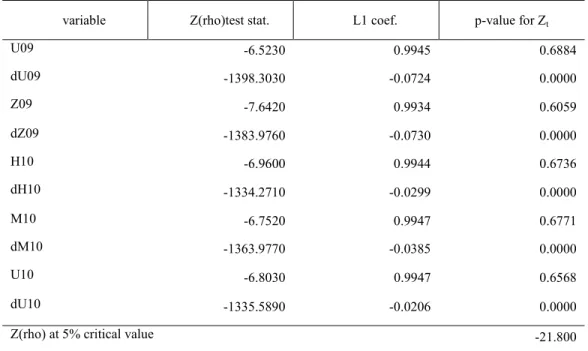
Table 1: summary of main values for variables at their levels and first differences
variable Z(rho)test stat. L1 coef. p-value for Zt
U09 -6.5230 0.9945 0.6884
dU09 -1398.3030 -0.0724 0.0000
Z09 -7.6420 0.9934 0.6059
dZ09 -1383.9760 -0.0730 0.0000
H10 -6.9600 0.9944 0.6736
dH10 -1334.2710 -0.0299 0.0000
M10 -6.7520 0.9947 0.6771
dM10 -1363.9770 -0.0385 0.0000
U10 -6.8030 0.9947 0.6568
dU10 -1335.5890 -0.0206 0.0000
Z(rho) at 5% critical value -21.800
Source: analysis by the author adapted from STATA
The values extracted from out t-test for variables in their level are higher than critical values, with significant p values, therefore, we accept the null hypothesis. Variables are non stationary in their levels, then we test the first differences of the variables. These turn out to be stationary, given their small p values. Hence, we can conclude that all variables are integrated of order 1 , I(1), considered for random walk series. From this step, we proceeded with cointegration analysis. In order to test whether the series are cointegrated, the cointegration regression (Best, 2008).
Y=α+ßX+ Zt
sta-tionarity. To validate the model, we test residuals (z) that happen to be stationary, again, due to small p values, we reject the null.
Table 2: summary of main values for cointegrated variables
variable Z(rho)test residual L1 coef. R-square Root MSE
regu09z09 -30.2020 0.9523 0.9635 0.0173
regz09h10 -124.4120 0.7567 0.9865 0.0109
regh10m10 -25.6170 0.8569 0.9891 0.0129
regm10u10 -31.4850 0.9382 0.9929 0.0120
regu10z10 -37.5570 1.0267 0.9931 0.0125
Z(rho) at 5% critical value -14.1000
Source: analysis by the author adapted from STATA
The second step of analysis is the construction of ECM (Error correction model) based on the long run dynamics, we study short term movements. Results of cointegration analysis are generated in STATA. We can estimate, that our correction from one observation to another ranges from 4.5%-13.2%. As stated in Best (2008), Granger causality can be ascertained in the ECM framework by regressing each time series in differences form on all time series in both differenced and level form. If an EC representation is appropriate, then in at least one of the regressions :
The lagged level of the predicted variable should be negative and significant
The lagged level of the other variable should be in the expected direction and significant. Our outputs confirm this assumption.
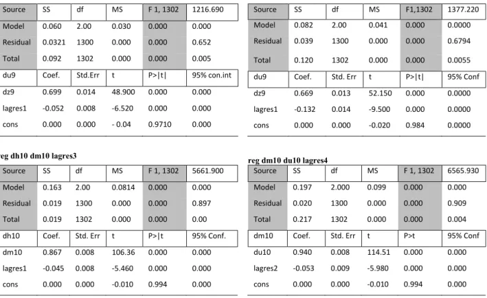
Table 3: ECM
variable coef. R-square Root MSE
regdu09zd09lagres1 0.6998 0.6518 0.0050
regdz09dh10lagres2 0.6695 0.6794 0.0055
regdh10dm10lagres3 0.8669 0.8970 0.0038
regdm10du10lagres4 0.9401 0.9099 0.0039
Source: author adapted from STATA
∆Yt = β₀∆Xt-1 - β₁Zt-1
As we can read from the equation above, deviations from the previous period will always be corrected, on a very short term. Thus, the best predictor of the value at t is the value at (t-1). For a Thus, the best predictor of the value at t is the value at (t-1). For a model to be valid, ß2 must be
negative. All the ß2 (applied on the four five series) are negative. Hence, we conclude our model
is valid.
4.2. Results of financial performance
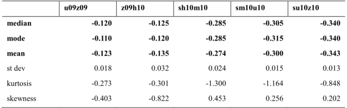
From this point onwards, we continue modeling in Excel, where we use the MSE coefficients adjusted to appropriate time horizon. From our analysis, we could extract standard deviation for the entire trading period of 21 days, in future steps of our analysis; however, we will work only on a daily time frame. In order to create a valid model, we must first assume an approximate normality of distribution.
we can afford to consider the data being approximately normally distributed and we deduce the daily standard distribution value for our further research.
Table 4: descriptive statistics for
u09z09 z09h10 sh10m10 sm10u10 su10z10
median -0.120 -0.125 -0.285 -0.305 -0.340
mode -0.110 -0.120 -0.285 -0.315 -0.340
mean -0.123 -0.135 -0.274 -0.300 -0.343
st dev 0.018 0.032 0.024 0.015 0.013
kurtosis -0.273 -0.301 -1.300 -1.164 -0.848
skewness -0.403 -0.822 0.453 0.256 0.202
Source: analysis by the author
σ day=σ period*√no of days where no of days= 22.
From this formulation, we obtain daily standard deviation for every spread series that we analyze. In order to have a valid mean, we use previous daily observations (no of observations=45 per day). We create a model flexible enough to simulate different standard deviation parameters and also the related numeric outcomes. Our spreadsheet models both strategies, range trading with and without reversals. We will generate results for the four spread series that are object of our analysis. The return will be estimated according to the capital employed (margins deposited by the broker), first without, then with a transaction cost.
likely to open trades more often, but the system can give us less objective criteria and sometimes trigger trades on the false signals.
Table 5: simulated results for respective thresholds
1.5σ P/L rev.3 P/L no revers4
no.
trades5 cost5 P/L no exec.risk6 P/L bid ask7 net P/Lbid ask8
s1 1,412.50 662.50 24.00 96.00 566.50 87.50 -8.50
s3 1,050.00 437.50 24.00 96.00 341.50 62.50 -33.50
s4 1,150.00 500.00 26.00 104.00 396.00 0.00 -104.00
s5 1,087.50 550.00 22.00 88.00 462.00 50.00 -38.00
total 4,700.00 2,150.00 96.00 384.00 1,766.00 200.00 -184.00
return9 185.895% 21.05% -19.37%
1.8σ P/L rev. P/L no revers
no. of
trades Cost P/L no exec.risk P/L bid ask net P/Lbid ask
s1 1,212.50 575.00 20.00 80.00 495.00 100.00 20.00
s3 825.00 350.00 18.00 72.00 278.00 100.00 28.00
s4 825.00 350.00 19.00 76.00 274.00 25.00 -51.00
s5 750.00 362.50 15.00 60.00 302.50 37.50 -22.50
total 3,612.50 1,637.50 72.00 288.00 1,349.50 262.50 -25.50
Return 142.053% 27.63% -2.68%
2σ P/L rev. P/L no revers
no. of
trades Cost P/L no exec.risk P/L bid ask net P/Lbid ask s1 1,137.50 537.50 16.00 64.00 473.50 162.50 98.50
s3 725.00 250.00 16.00 64.00 186.00 100.00 36.00
s4 550.00 212.50 12.00 48.p0 164.50 62.50 14.50
s5 575.00 287.50 11.00 44.00 243.50 62.50 18.50
total 2,987.50 1,287.50 55.00 220.00 1,067.50 387.50 167.50
return 112.368% 40.79% 17.63%
2.5σ P/L rev. P/L no revers
no. of
trades Cost P/L no exec.risk P/L bid ask net P/Lbid ask
s1 937.50 437.50 13.00 52.00 385.50 162.50 110.50
s3 400.00 62.50 11.00 44.00 18.50 12.50 -31.50
s4 550.00 162.50 11.00 44.00 118.50 62.50 18.50
s5 550.00 262.50 10.00 40.00 222.50 37.50 -2.50
total 2,437.50 925.00 45.00 180.00 745.00 275.00 95.00
return 78.421% 28.95% 10.00%
3σ P/L rev. P/L no revers
no. of
trades cost P/L no exec.risk P/L bid ask net P/Lbid ask
s1 762.50 312.50 9.00 36.00 276.50 112.50 76.50
s3 350.00 112.50 8.00 32.00 80.50 62.50 30.50
s4 387.50 87.50 8.00 32.00 55.50 37.50 5.50
s5 375.00 150.00 7.00 28.00 122.00 25.00 -3.00
total 1,875.00 662.50 32.00 128.00 534.50 237.50 109.50
return 56.263% 25.00% 11.53%
3 Potential would be P/L realized if a trade at every closure would start immediately another in reversed direction 4 P/L simulated if trades are separated and opening of a new one does not occur at the same time as closing of previous one 5 Number of trades under preset conditions
6 P/L no reversals-cost
7 P/L simulated if we create a half tick cushion to avoid execution risk, hence we reduce our profits in a calculated manner 8 P/L bid/ask- cost
9
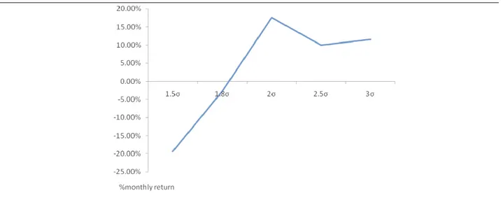
From the above noted returns, we can conclude also from Chart 7 that our profitability peaks up when a trade is triggered under 2σ measure.
Chart 7 Graph of returns
Source: author adapted from EXCEL
For illustration, we may compare this system to randomly picked systems, hence our system would fall into a half with higher profitability, maintaining a reasonable risk profile.
Table 6: day trading returns
System Daily return Monthly return
running up10 0.48% 10.58%
channel breakout11 0.44% 9.66%
broadening bottom12 1.26% 30.08%
15 minute breakout13 0.80% 18.21%
CARC (Close above resistance
confirmed)14 0.60% 13.39%
Source: www.day-trading.in
10 Identifies stocks with abnormally high upward, spots the trend early and follows the trend 11 Security that breaks away from a range of prices is usually trades in
12 This formation is typical with the successively higher highs and lower lows, which form after a downward move. Usually, two higher highs
between three lower lows form the pattern, which is completed when prices break above the second higher high and do not fall below it
5. Conclusions
Our study aimed to simulate the trading environment of the short term interest rates futures, while studying the movement of pairs of contracts (spreads). We looked at calendar spreads, considering the contracts of different expiries and detected the short term departure from the equilibrium in the value of the spreads. By taking two simultaneous positions on one instrument at different points of the yield curve, we reduced substantially the risk of “being on the wrong side of the market”, one position, be it long or short, will serve as the hedge to the opposite position on the other contract, long trade will be off-set by the short and vice versa. Contrary to outright trading, spread trading will hence study the relative value of the contract.
We used time series statistical analysis to prove that individual series did not fit to linear trend, on contrary they resembled to random walk, we proved they are non stationary variables with a unit root. Having reached this result, we proceeded with a study of cointegration, which refers to linear combination of non stationary variables. Cointegration simulated the existence of a long run equilibrium to which the system converged over time. In the later part of analysis, we constructed the error correction model, based on the long run dynamics, we studied short term movements. We ran this testing on the STATA. Four out of five spreads proved to be stationary and derived from cointegrated series.
In our case, we estimated one month period, following the rollover, from the 15th of Eune 2009 until the 14th of Euly 2009. A total number of observations is 1304. We managed to develop a set of objective criteria that resulted into a sustainable investment strategy, considering transaction costs and execution risks. We simulated the threshold of spread which would trigger the change in positions across contracts and maximize profits as 2 standard deviations of spread.
forget that markets are constantly changing and this feature invites us to test periodically the match of our results on the sample.
We investigated the trade number and profit constraint issues using data generated from a cointegration model. We also observed that using alternative values for opening and closing our trades affects in a large extend profitability of the system as well as a number of trades. Our simulation enhances control over trading by complying to a given model with the prescribed parameters. This filters out data noise that take place if trading rule hasn’t been clearly set. Our analysis shows that profitability of the spread trading depends upon using weighting rules, minimum profit hurdles and open/ close criterion that reflect the short term behavior of the component contracts. Any trading opportunity is a compromise between trading frequency, duration and per trade profitability. Spread trading result depends on achieving a suitable mix between these components.
The major value of the paper resides in the structuting a valid strategy in intraday spread trading based on setting the threshold to trigger and close a trade while maximizing our profit. We take a side of a risk-averse investor and this argument encourages us to proceed with building a valid model.
Algorithmic trading, often called program trading, is the computerization of futures trading where software replaced the trader in decision making. This type of trading has seen a massive growth in the past two decades, especially since hedge funds, started to cover such a wide scope of markets that it became impossible to punctually analyze in detail every trade. We can use our model, once proved profitable, to reduce uncertainty of human aspect from decision making. We can incorporate the orders into software that executes our trades when the parameters are reached. Several softwares offer packages including this feature, such as TT, X Trader, E Trader...
6. References
AIKIN S. (2006). ,
Wiley
ALEXANDER C., (1999): Optimal Hedging Using Cointegration, , !, pp. 2039-2058
ANAT A.& PFLEIDERER P., (1988). A theory of intraday patterns: volume and price variability,
" , #(1) , pp. 3-40
BEKIROS S.,& CEES D., (2008). The relationship between crude oil spot and futures prices:Cointegration, linear and nonlinear causality, Center for Nonlinear Dynamics in Economics and Finance (CeNDEF), Department of Quantitative Economics, University of Amsterdam, $ $ 30, pp. 2673–2685
BERNOTH K., & HAGEN E., (2003). The performance of the Euribor futures market: efficiency and the impact of ECB policy announcements, Bonn
BEST R., (2008). An introduction to error correction models, Oxford Spring School for Quantitative Methods in Social Research
BEOLBERG A., (2001). Price relationship in the petroleum market: an analysis of crude oil and refined product prices, Foundation for research in Economics and Business Administration, Bergen
BOSSAERTS P.,(1988). Common nonstationary components of asset prices. %
$ & ' #((3), pp. 347-364
BROCK W.,& LAKONISHOK E., (1992). Simple technical trading rules and the stochastic properties of stock returns, % , )!(5), pp. 1731-1764
BROWN D.,& Eennings R., (1989). On technical analysis, " , ((4 ),
pp. 527-551
CAROL A., (1999). Correlation and cointegration in energy markets, Managing Energy Price Risk (2nd edition), RISK Publications, pp. 291-304
CLEMENTS M.& TAYLOR N., (2003). Evaluating interval forecasts of high-frequency financial data, % $ , #*(4), pp. 445-456
CLEVELAND W.,& DELVIN S., (1980). Calendar effects in monthly time series: detection by
spectrum analysis and graphical methods, E ,
COX C., (1976). Futures trading and market information, % $ *)(6), pp. 1215-1237
COX E., & INGERSOLL E.,& S. A. ROSS S., (1985). A theory of the term structure of interest rates, $ , , pp. 385-407.
Day trading systems, & (2005, Eanuary, 18) retrieved November
11, 2005 from http://www.day-trading.in/news/news_18012006.html
DOLADO E.,& GONZOLO E.& MARMOL F., (1999). Cointegration, Department of Economics, Department of Statistics and Econometrics, Universidad Carlos III de Madrid DUNIS C.,& LAWS E. & EVANS B., (2005). Modelling and trading the gasoline crack spread:a non-Linear Story, CIBEF+ and Liverpool Eohn Moores University
DUNIS C.,& LEQUEUX P., (2000). Intraday data and hedging efficiency in interest spread
trading, $ % 6, pp. 332-352
ENGLE R.,& GRANGER C., (1987), Co-integration and Error Correction: Representation, Estimation, and Testing, $ (2). pp. 251-276
EURONEXT. LIFFE, (2004). Interest Rate Product Management 3855, Liffe. Retrieved from http://www.euronext.com/fic/000/010/894/108942.pdf
FAMA E.,& FRENCH K., (1992). The Cross-Section of Expected Stock Returns. % )!(2), pp. 427–465
FOSTER F.D., & VISWANATHAN S., (1993). Variations in Trading Volume, Return Volatility and Trading Costs: Evidence on Recent Price Formation Models, % , )*, pp.
187-211
FULLER, W., (1996). Introduction to Statistical Time Series, Second Edition. Eohn Wiley, New York.
GATEV E.,& GOETZMANN W., ROUWENHORST G., (2006). Pairs Trading: Performance of a Relative-Value Arbitrage Rule, " , #+(3), pp. 797-827
HAIGH M. ,& HOLT M., (2000). Hedging multiple price uncertainty in international grain trade,
% $ , *((4), pp. 881-896
HANSELL, S., (1989). Inside Morgan Stanley's Black Box, " , May,
pp. 204
HARRIS L., & SOFIANOS G., & Eames E. SHAPIRO E., (1994). Program trading and intraday volatility, " , Vol. !(4), pp. 653-685
HARRISON P. , & STEVENS C.F., (1976). Bayesian Forecasting, %
. Series B (Methodological), *(3), pp. 205-247
HEIBERGER R. ,&. TELES P., (2002). Displays for direct comparison of ARIMA Models , , ,(2), pp. 131-138
HENDRY D. F., (1999). Explaining Cointegration Analysis: Part I, European University Institute, Florence
HULL, E. C., (2011).- - & " " , Pearson / Prentice Hall; 8 edition
CHAVAS E.P., & HOLT M., (1991). On nonlinear dynamics: the case of the pork cycle,
% $ , ! (3) pp. 819-828
CHORDIA T. ,& ROLL R., (2001). Market liquidity and trading activity, % , ,(2), pp. 501-530
CHUA C.T. ,& KOH W. & RAMASWAMY K., (2004). Profiting from mean-reverting yield curve trading strategies, Singapore Management University
EENS S. ,& WHALEY R., (1990). Intraday Price Change and Trading Volume Relations in the Stock and Stock Option Markets, % , ) (1), pp. 191-220
KAWALLER I. ,& KOCH P. & LUDAN LUI, (2002). Calendar spreads, outright futures
positions, and risk, % " " pp. 59 – 78
KAWASAKI Y., & TACHIKI S., & UDAKA H., & HIRANO T. (2003). A characterization of long-short trading strategies based on cointegration, $$$
' ' $ , pp. 411-416
KAWASAKI Y., & YOSHONORI & TACHIKI S. & UDAKA H., (2009). A Characterization of Long-Short Trading Strategies Based on Cointegration, Department of Prediction and Control, The Institute of Statistical Mathematics
KIM Ch.. E. ,& NELSON Ch., (1997). Testing for mean reversion in heteroskedastic data II: Autoregression Tests. % $ ##, University of Washington