'-4
O
SEMINARIOS DE ALMOÇO
i
O
FUNDAÇÃO
DA EPGE·
O
GETUUO VARGASO
O
O
O
O
O
Can°
macroeconomic variables
O
o·
account for the term structure of
o
o
sovereign spreads? Studying the
o
o
Brazilian case.
o
o
o
o
o
o
MARCO MATSUMURA
o
o
(lPEA)
O
o
O
O
O
O
Data: 12/08/2005 (Sexta-feira)
O
O
Horáriq: 12 h 15 min
O
O
,.".
Local:O
Praia de Botafogo, 190 - 110 andarO
FGV
Auditório nO 1O
O
EPGE
Coordenação:o
o
o
o
o
o
o
o
o
o
o
o
o
o
o
o
o
o
o
o
o
o
o
o
o
o
o
o
o
o
o
o
o
o
o
o
o
o
o
o
o
o
o
o
o
o
o
o
o
Can Macroeconomic Variables Account for the Term
Structure of Sovereign Spreads? Studying the Brazilian Case
Marco Matsumura 1,
Ajax Moreira2
June 2005
1.lntroduction
This article develops a model combining term structure and vector autoregressive
models to analyze sovereign and domestic term structure of interest rates. The
model is based upon the articles by Ang and Piazzesi (2003) and Ang, Oong and
Piazzesi (2005). One distinctive feature brought by those articles was to allow the
possibility of incorporating macroeconomic variables as state variables alongside
the latent state variables of the traditional term structure models. The joint behavior
of the yield curve and macroeconomic variables permits the study of public policy
effects on the yield curve and vice-versa. Oiebold, Piazzesi and Rudebusch (2005)
argues that," From a macroeconomic perspective, the short-term interest rate is a
policy instrument under the direct control of the central bank, which adjusts the rate
to aéhieve its economic stabilization goals. From a finance perspective, the short
rate is a fundamental building block for yields of other maturities, which are just
risk-adjusted averages of expected future short rates."
The idea of Ang and Piazzesi' s work is to use a discrete timespecification of an
Affine term structure model (se e Ouffie and Kan 1996 for instance) which is at the
same time a Vector Autoregressive (VAR) model. Then, this model can be
extended with the addition of macroeconomic variables as in the Macro VAR
literature, without loosing the affine characterization. Also, the no-arbitrage
I DimaclIPEA: marcom@ipea.gov.br
condition is pmsent in the model, a restriction not necessarily enforced in Macro
VAR models. Finally, ali the flexibility and advantages of the VAR model are
retained. Variance decompositions and impulse response functions can be easily
calculated.
Thus, this line of research can take advantage of using the tools and results of
Macro VAR síudies and Affine term structure models one into the other to
investigate questions of interest in both public policy and asset pricing.
Our article extends the work by Ang and Piazzesi in a number of ways. First, we
propose a simplified specification and a method of estimation. This was motivated
by the recognition after various experimentations with both Maximum Likelihood
and Monte Carlo Markov Chain that the estimation process turns out to be very
delicate and di'fficult, which is caused by the high dimensionality and high
non-linearity of the rnodel.
This proposal is a multidimensional affine model for the yield curve that is as easy
to estimate as usual empirical procedures. However, we must say that this
simplification had the effect of reducing the possibility of discussing monetary
policy questions, and so we concentrate only on the relation between
macroeconomic variables and the term structure of interest rates and of credit
spreads.
Second, we developed an extended model incorporating the possibility of default
and a credit sp:read variable. This is a version of Duffie and Singleton' s (1997)
reduced model. Here a question of central interest is trying to understand how the
sovereign spread due to defaultis related to macroeconomic variables (and to
monetary policy in the general model).
The third contribution was to present and compare several results for different
specifications of the model for US Treasury, swaps from BM&F (Brazilian Future
Markets Exchange), and emerging market sovereign bonds. We remark that the
simplification of the estimation process allowed the addition of the short spread in a
O
O
O
O
O
O
O
O
O
O
O
O
O
O
O
O
O
O
O
O
O
O
O
O
O
O
O
O
O
O
O
O
O
O
O
O
O
ü
o
o
o
o
o
o
o
o
o
o
o
o
o
o
o
o
o
o
o
o
o
o
o
o
o
o
o
o
o
o
o
o
o
o
o
o
o
o
o
o
o
o
o
o
o
o
o
o
model that would otherwise have a too high dimensiono And credit risk is a
fundamental variable concerning ali emerging countries.
,
To the authors' knowledge, in the existing models in the credit risk literature, the
spread only reacts to the default free reference short-term interest rate. For
example, Ouffie, Pedersen and Singleton (2002) study the dynamics of the
Russian term structure of interest rates. They calculate the model implied
instantaneous spreads due to credit risk and compute via an illpulse response
function how it relates to the Govemment reserves or to the price of the petroleum.
However, in their model, macroeconomic variables play no direct role in the
determination of the spread dynamics.
Thus, the present study focuses on measuring the effects of macroeconomic
shocks over the term structure of interest rates and of credit spreads. Ang and
Oong and Piazzesi (2005) take full account of the monetary issues, using MCMC.
We also tried to used MCMC besides Maximum likelihood and intend to tackle this
problem in future work.
In the following, we present the AP' s general framework and after that we show
the specific choices where we ran the estimations.
2. Affine Term Structure Model with Macro Factors
2.1 Inilial comments
In AP' s approach, the economy is represented through the state variables X that
have observable macro components m and monetary or financiai components u.
The dynamics of X is described by a VAR, and the monetary policy by the relation
between the short rate
r
and the state variables of the economy. A key idea inAP' s article is to make that relation a combination of the Taylor' s rule li
=
ao +a1 fot + Vt , where
Pt
is a vector of observable macro factors and ~ representscomponents not explained by macro factors, and of the affine term structure
equation Il = bo + b1 XUt, where Xllt is a vector of latent factors, that is, n = do + d11
Then, the model will be affine: the relation between the interest rates of chosen
maturities Y and the state variables is linear given the parameters. So Y and X
have the same dynamic properties from the time series point of view. The
dynamics of X is given a priori, and its parameters are found using a historical
series of Y. Change of variables is used to obtain Y' s distribution in terms of
X' s.
Our proposal departs from Ap'swhen we consider that the short rate describes the
state of the economy and hence is a state variable, and when we represent the
monetary polic:y in the usual form in the VAR Iiterature, identifying the
contemporary r,elations between the state variables. Then, we do not need to
invert the function from X to Y to make the estimation of ali parameters at once.
With those modifications, one looses the possibility of describing some aspects of
the monetary condition that would exist in a model with more unobservable latent
monetary factors. On the other hand, this model is much easier to be estimated.
And as we will see later on, even with our assumptions, the estimation of the risk
premium will be far from being a straightforward task.
In our approach, we directly estimate the short rate first to fix some of the
parameters. This is possible because we have set
cb
=°
and d1 = (1,0, ... ,0) andincluded rt as one of the state variables.
2.2 State variables
The state variabi'es will have the following dynamics:
The financiai fac:tors li and St and the macro variables Illt of the vector
Xt
are AR(1)factors, but the macro factors can include lagged factors of any order.
2.2 The Pricing Kernel
Bonds in our economy will be priced using the Martingale approach of Harrison
and Kreps (197'9). Assuming no arbitrage, we know that the existence of an
O
O
O
O
O
O
O
O
O
O
O
O
O
O
O
O
O
O
O
O
O
O
O
O
O
O
O
O
O
O
O
O
O
O
O
o
;0
O
O
O
O
.0
O
O
O
O
O
O
O
O
O
O
O
O
O
O
O
O
O
O
O
O
O
O
O
O
O
O
O
O
O
O
O
O
O
O
O
O
O
O
O
O
O
equivalent martingale measure Q is guaranteed. The price at time t of an asset that
pays no dividend is
Denoting by 1;t the Radon-Nikodym derivative
dQ
=çr
dP
Using a discrete time analogy of the Girsanov's theorem, we assume that 1;t follows
the process 1;t+1 =1;t exp(-O.5Àt*Àt -ÀtEt+1), where Àt represents time-varying market
prices of risk associated with the sources of uncertainty EI' We follow the literature
specifying the market prices of risk as an affine process: Àt =Ào +À1
x..
The pricing kernel is defined as mt = exp(-rt) 1;t+1 l1;t.
2.3 Pricing of bonds
Using the pricing kernel, the price of a (n+1 )-period bond will be:
p;+1 = Et (mt+1 P:I )
Choosing rt = õo+õ 1Xt, the price of the bond will be Affine:
p/
n
=exp(An
+ Bn
Xt)Then, it can be shown that the coefficients
An
andSn
can be calculated recursivelythrough the following relations:
(2)
(3)
~+I =-õo+
A"
+(,u' -~V)B" +0.5 B~ VV B" (4)B"+I =-Õ1+(<j>' -~V)Bn (5)
The n-period Yield is:
y:
=
-Iogpt" In=
An + Bn XtAn =-A"/n
Bn =-S"/n
(6)
or
~
=[:IJ =
[~IJ+[~IJx,=A+
BXtyn
,
Ali Bn(8)
2.4 Introducing the Spread
An important oamponent in the term structure of emerging countries is the spread
due to the possibility of default of the bond. In the /iterature, two /ines of research
have developed regarding this question: the structural and the reduced models.
We choose to implement a discrete version of the reduced model as presented in
Duffie-Singleton (1999):
• Let hs be the conditional probability at time s under a risk neutral probabi/ity
Q of default between s and s+1 given the information available at time s in
the event of no default by s.
• Let <l>s be the recovery upon default.
• Let Vtdenote the price of a defaultable claim.
Then:
Using the Recovery of Market Value hypothesis Ef(<pS+l)={l-LJEsº(VS+l)' where
Ls denotes the loss rate upon default, it follows that:
Or,
v;
=
EF(v;+I)((1-h,)e-n + h,e-r'(1- L,))=
E? (V;+I )e-r' (1-h/L,)
Now, note that exp(-htLt) "" 1- htLt. If we set that relation to be an equa/ity (just
redefine Lt), we will have
V;
= E,º(V'~I
)exp(-~
+ h/L, )as in the continuous case.
O
O
O
O
O
O
O
O
O
O
O
O
O
O
O
O
O
O
O
O
O
O
O
O
O
O
O
O
O
O
O
O
O
O
O
o
o
o
o
o
'0
O
O
O
O
O
O
O
O
O
O
O
O
O
O
O
O
O
O
O
O
O
O
O
O
O
O
O
O
O
O
O
O
O
O
O
O
O
O
O
O
O
O
Thus, the affine setting can be maintained. We call the additional term St=htLt the spread due to default. The spread St will be another ~tate variable.
If we denote by l'~the price of a defaultable bond, then using the equivalent martingale measure, we have that
n+1 - Eº[ ( ) n ]
PI - I exp -~ -SI PI+1 •
Moreover, the pricing kern,el and the pricing equation can be found using equations
that bear resemblance to the previous ones.
2.5 Likelihood
The likelihood is the density function of the joint distribution of (Xt , Yt). To calculate it, we will invert those variables in terms of (Xt, Ut), that is:
We considered the risk free short rate n as measured without errors, and that other
yields have an i.i.d. measurement error Ut.
Chen and Scott (1993) first introduced the idea of adding measurement errors in
some yields. The number of yields measured without error is the same as the
number of latent state variables. Then, each additional yield has to come with a
measurement error Ut to make them compatible with the previous yields. The error
Ut is independent of ali other variables.
Using (*) and the know distribution of (Xt , Ut), applying change of variable formula
we have:
L(V)
=
fX(J.1,<j>,V)+ fu{J.t,<j>,V,À,o,À,1) + fofx(X I
I
XI_I) =-.5{(T -1 )log(det(VV' ))+L~=2
(XI - fl-iflXr-1 )'(VV'-I )(Xr - fl-</lXt-I)}fu(u;)
=
-O.5{(T -1)I:I
a/
+I~=2
I:I
(:"~2
}
I
2.6 Estimatiorn
The log likelihood is the sum of 3 terms, fx(J-l,<j>,V), fu(Jl,<j>,V,ÂQ,À1 ,a), fo, where:
1) fo =0 for det(J)=1
2) The functions A(.), B(.) can be reparameterized with no loss of generality making
," • Ã' Ã" , Ã' d 'I * ÷ Ã"
AO=J1-''QV,,,,=<j> -,.,V,an 11.="0"" ,so
3) In the func:tion fu{.) the parameters ai can be substituted by its maximum
likelihood estimator
a\V,À*)=
"K
(y,i -A(V,À*)-B(À*)iI ~=l
T
4) Thusfu(Jl,<j>,V,ÂQ,À1,a) can be reparameterized with no loss as fu(À*,V).
Considering iterns 1-4, L('I') = fx(Jl,<j>,V)+ fu(À*,V).
The maximization problem was solved in a conditional way making
ma~{'I') = maxILcp.v fx(Jl,<j>,V) + max fu{À *IV)
The first problem, maximizing fx, corresponds to the estimation of the VAR model, and the second one to a non-linear maximization in the vector À *.
Moreover, using simulated data we concluded that the use of conditional
maximization caused negligible alteration in the likelihood.
In this way, we greatly simplified the estimation process, reducing the dimension of
the maximizati()n. So, one state variable is always the short rate, considered
measured without error. Macro and spread factors can be added depending on the
specification.
We remark that the longer rates (considered as measured with errors) are needed
to identify the constant risk premium and the constant termo It can be show that an
estimation using only the state variable ( cannot distinguish the long-term mean
short rate from the risk premium.
O
O
O
O
O
O
O
O
O
O
O
O
O
O
O
O
O
O
O
O
O
O
O
O
O
O
O
O
O
O
O
O
Q
O
O
O
O
o
o
o
o
o
{)o
o
o
o
o
o
o
o
o
o
o
o
o
o
o
o
o
o
o
o
o
o
o
o
o
o
o
o
o
o
o
o
o
o
o
o
o
o
o
o
o
o
The use of an observable short rate is not a relevant restriction since in the affine
model, yields of longer maturities are linear functions Y=BX+A of the state variable.
Since the characteristic roots of the dynamics of Y and X are the same, only
differences of scale distinguishes both processes and the estimation should not be
significantly different.
Also, we remark that the effect of each risk premium over the likelihood is different.
Thus, one may be easier to estimate than the other.
3. Using the Model
3.1 Initial comments
To show the f1exibility of this model and the difficulties of the estimation of the risk
premiums, we considered 4 specifications. The first model (A), is a model that
uses swap rates with various maturities from BM&F (Brazilian futures exchange) to
study the Brazilian market. The second, Model (8) is an extension of the previous
one that includes a macro variable - the log of the Brazilian Real R$/US$
exchange rate - to analyze the interaction between nominal exchange rate
shocks and interest rates. The third, model (C), is similar to the first model, but is
estimated using constant maturity interest rates of the American market calculated
by the FED. Finally, the fourth model (D) relates the term structure of the Brazilian
sovereign spread with the American interest rates and with a measure of
vulnerability of the debt of the Brazilian economy.
The 4 specifications utilize 2 sets of data. The first one, utilized by (A) and (B),
contain the 1 day swap e swaps of selected maturities - 1,2,3,6,9, 12, 18,24
and 36 months - produced by the BM&F, covering the period from 01/0112001 to
30/05/2005 and containing 1035 daily-observations. The second set, utilized by the
other specifications, contain: 1) constant maturity interest rates calculated by FED
of maturities of 1 month and {1, 5, 10, 20} years; 2) Brazilian sovereign spread
form Republic of Brazil; and 3) the logarithm of the exchange rates deftated by the
IPCA3 (Brazil' s Consumer Price Index).
In ali cases the parameters were estimated by the maximum ikelihood criterion4 .
The optimization was repeated from 10 initial points chosen at random in a relevant
region. An index of multiplicity of modes IMM was defined as the standard
deviation of the Loglikelihood (LL) of the 10 optimization trials.
To test he pmdictive capacity of the models, the last 100 observations were taken
away from the estimation sample. The lag of the VAR model is defined in monthly
terms, but we wanted to use the entire daily measured sample. Our approach was
to consider a lag of 21 days - the medium number of commercial days in a month
- and to esttmate the models as though the daily data were 21 replications of
monthly data.
To validate ithe estimations, a simulation exercise was realized with the
specifications 1 and 2. In those cases, 100 samples where generated conditioned
to the value of the estimator (1j) obtained with real data, and repeating the
optimization exercise with 10 trials as already described. Thus, a sample of the
distribution of the estimators of the parameters where obtained. In what follows,
each specification is described with more details along with its corresponding
results.
In ali cases, the same model is estimated, namely equations (1) and(8), where the
specifications are characterized by the definition of the vectors (Xt,Yt).
3.2 Case A: The term structure of interest rates in Brazil
This model relates the dynamics of the short rate X, the 1-day swap of the BM&F,
with the term structure Y of swaps of other maturities. It is the simplest
specification., for the stochastic process that has only 1 quantity - the 1-day rate
- and contains only 2 risk premium parameters, the constant one and the one
proportional to levei of the short rate. Figure 1 shows the trajectory of those rates,
3 we supposed that the leveI of IPCA was Constant each day over a month.
4 Using the fininsearch routine from mathlab 6.5.
O
O
O
O
O
O
O
P
O
O
O
O
O
O
O
O
O
O
O
O
O
O
O
O
O
O
O
O
O
O
O
O
O
O
O
o
o
o
o
o
o
o
o
o
o
o
o
o
o
o
o
o
o
o
o
o
o
o
o
o
o
o
o
o
o
o
o
o
o
o
o
o
o
o
o
o
o
o
o
o
o
o
o
where 1he elevated correlation among them can be seen. In fact, we found that the
first component of the canonic decomposition of the correlation matrix of those
rates explains 95% of the total variability of the series.
The table A 1 shows the value of the log-likelihood (LL) at the optimal point and the
index of multiplicity of modes, which featured a positive value. After that, statistics
relative to the simulation exercise are shown: The mean value of the LL
conditioned to the true value of the parameters, and then conditioned to the optimal
value in each estimation. The mean value of the IMM is shown too, and a measure
of the variability of the LL conditional to the estimated value of the parameters.
Tab A-1: Estimated and simulated 109 likelihood Estimation Simulation
LL IMM M(LLI'I') ~(LLIt{! ) M(IMM) ~D(LLIt{! )
-2121.C 19.8 -1604.2 -1603.1 3 9.1
The results show that the LL has multi pie modes, and that even so the adopted
optimization algorithm obtains the minimum value, as can be seen in the
comparison between the mean value of the LL conditioned to the true value of the
parameters and to the estimated value. Table A2 shows the estimated values of
the parameters of the model and the corresponding estimated standard deviation.
Moreover, it shows the simulated results, the value utilized in the generation of the
samples, and the mean value of the t{!, and the corresponding standard deviation.
Finally, it shows the correlation between the estimators.
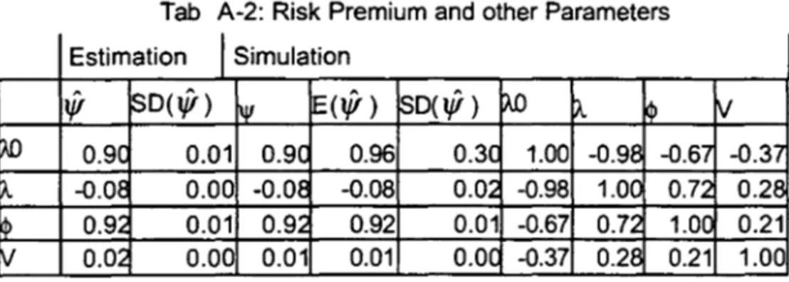
Tab A-2: Risk Premium and other Parameters Estimation
I
Simulation'"
~D(t{! ) ~ ~(t{! ) SD(t{! ) f>.O ~!t
V~ 0.9C 0.01 0.90 0.96 0.30 1.00 -0.98 -0.67 -0.37 ~ -0.08 0.00 -0.08 -0.08 0.02 -0.98 1.0C 0.72 0.28
~ 0.92 0.01 0.92 0.92 0.01 -0.67 0.72 1.00 0.21 ~ 0.02 0.00 0.01 0.01 O.OC -0.37 0.28 0.21 1.00
The results show that the parameters are measured with precision, and that the
mean value of t{! is similar to the true value of the parameters, as well as the
estimation of its standard deviation. This happens in spite of the estimated high
the values of the observed and the model predicted rates in the last period, as well
as the mean value of this quantity predicted in the simulation exercise. It then
shows the results corresponding to the parameters O' relative to the error in the
equations xx.
Tab A-3: Term in the final Period and a
T Y(T,.)
la
~ Y M(Y) SD(Y) O' M(cY ) ~D(cY )
1 0.19 0.19 0.2059 0.0033 0.01 0.0046 O
~ 0.19 0.20 0.208 0.0033 0.01 0.0085 0.0001
0.19 0.20 0.2101 0.0033 0.01 0.0156 0.0001
E 0.19 0.20 0.216 0.0033 0.02 0.0254 0.0005
~ 0.19 0.21 0.2213 0.0033 0.03 0.0239 0.0003
1~ 0.19 0.22 0.2262 0.0033 0.03 0.0305 0.0002
1c 0.18 0.22 0.2346 0.0033 0.04 0.038€: 0.0003
2 0.17 0.23 0.241 0.0034 0.05 0.0491 0.0005
3{ 0.17 0.24 0.2478 0.0034 0.06 0.0613 0.0008
The results show that the term structure of these rates were not recuperated in the
last period - 30 of may of 2005 - possibly because of the atypical characteristics
of the term structure in Brazil caused by monetary policy. The results relative to the
para meter O' show that the estimator of this para meter was adequate in the
simulation exercise.
Next, table A4 presents the predictive capacity of the model through the Theil-U
statistics that measure the ratio between the standard deviation of the error of the
prediction and IOf the error ofthe random walk. The results show that the model has
predictive capacity - T -U less than 1 for prediction up to 3 months. The simulation
exercise shows that with simulated data, the model exhibits predictive capacity for
ali horizons, am:J that those statistics are measured with precision.
Tab A-4: Predictive capacity
T T-U (tlt) T-U (tlt-1)
MV M(.) DP(.) MV M(.) DP(.)
1.0e 0.27 0.32
o.oe
0 __ 46 0.93 0.002.0e 0.57 0.48 0.01 0.35 0.87 0.01
3.0e 0.92 0.61 0.01 0.51 0.80 0.01
6.0e 2.24 0.67 0.01 1.73 0.76 0.01
O
O
O
O
O
O
O
O
O
O
O
O
O
O
O
O
O
O
O
O
O
O
O
{)
O
O
O
O
O
O
O
O
O
O
O
O
O
o
O
O
O
O
O
O
O
O
O
O
O
O
O
O
O
O
O
O
O
O
O
O
O
O
O
O
O
O
O
O
O
O
O
O
O
O
O
O
O
O
O
O
O
O
O
O
O
9.0C 3.49 0.67 0.01 3.00 0.76 0.01 12.0C 5.03 0.67 0.01 4.55 0.73 0.01 18.0C 7.28 0.69 O.OC 6.87 0.73 0.01 24.0C 9.01 0.71 0.01 8.65 0.73 0.01 36.0C 10.58 0.71 0.01 10.31 0.73 0.01
Figure 1 below shows the impulse response function of the interest rates of various
maturities to the short rate shock. We see that the longe r the maturity of the rate,
the lower the effect of the shock .
Fig1: Impulse response functions and the trajectory of the rates in the period.
- m O 1.3
- m 1
1.1 0'_. m2
0.9 - m 3
0.7 - m 6
0.5 - m 9
- m 1 2
0.3 c, Ir.
1 2 3 4 5 6 7 8 9 10 - m 1 8 - m 2 4
3.3 Case B: Nominal exchange rate shock and term structure of interest rates in
Brazil
This specification extends the previous rrndel including the exchange rate, which is
a macro variable that is measured with daily frequency. With this specification we
intend to analyze the interaction between the financiai shocks over the interest
rates and exchange rate shocks. Being measured in nominal terms, the latter
variable captures aspects of the unbalances in the exchange market and in the
domestic nominal shocks. lhe tables in the following are similar to the tables
presented in the previous case, so we will comment only its results. In this case the
state variables are X=(short rate, log of the exchange rate R$/US$), the risk
premiums have 6 components, 2 relative to the constant component, and 4 relative
to components proportional to the state variables.
Tab 8-1: Estimated and Simulated 109 likelihood
Estimation Simulation
~L MM ~(LLI",) M(LLIl{t ) ,...,(IMM) ~D(LLIl{t)
The results of the table 81 show that the LL displays multiple modes and that the
optimization algorithm found the global optimum. The table 82 shows that the risk
premiums are estimated with precision according to the calculation carried out with
the Hessian of the LL. The simulation exercise shows conflicting results. The mean
value of the estimators
1jr
disagrees with the values with which the samples weregenerated, a fact confirmed by the value of the standard deviation of
1jr.
Theseresults characterize an identification problem in those models that suggests the
necessity of imposing restrictions over those parameters.
Tab 8-2: Risk Premium
Esnimation
I
Simulation1fI D.P 'V M(vI ) DP(vf ) ~(e) ~m A.(e,e) Ne,j) ~,e) Ni,j)
~(e) :3045 0.02 3.4e 1.10 2.5 1.00 0.02 -0.27 .0.12 -0.1/ O.OE
~O) -0.28 0.01 -0.2E -0.71 1.8~ 0.02 1.00 0.50 0.10 -O.7~ 0.21
Ne,e) -0.10 0.00 -0.1 C 0.12 004/ -0.27 0.50 1.00 0.35 -0.5': 0.3:<
Ne,j) -0.20 0.00 -0.2C -0.16 0.8 -0.12 0.10 0.35 1.00 0.1.11 -0.29
Ni,e) 0.01 0.00 O.O~ 0.12 0.0/ -0.17 -0.79 -0.53 0.14 1.0C -0.75
Ãij,j) -0.08 0.00 -O.OE -0.07 O.O~ 0.08 0.21 0.33 .0.29 -0.7e 1.0C
The T able 83 presents the rates of the last period and the parameter (j relative to
the error in the equation of the rates of various maturities. The results show that,
similarly to the previous case, the model could not recover, the term structure in
the last period, but the parameter (j looks adequately measured.
Tab 8-3: Term in the final period and cr
. Mat.
I
Y(T,.) crY Y M(Y) DP(Y) A
M(Ô') SD(cT )
(j
1 0.19 0.19 0.19 0.00 0.01 0.02 0.00
2 0.19 0.19 0.17 0.00 0.01 0.02 0.00
3 0.19 0.19 0.16 0.00 0.01 0.03 0.00
6 0.19 0.20 0.10 0.00 0.02 0.04 0.00
9 0.19 0.20 0.05 0.00 0.03 0.05 0.00
12 0.19 0.21 0.01 0.00 0.03 0.05 0.00
18 0.18 0.22 -0.08 0.00 0.04 0.07 0.00
24 0.17 0.22 -0.14 0.00 0.05 0.10 0.00
36 0.17 0.24 -0.23 0.00 0.06 0.12 0.00
O
O
O
O
O
O
O
O
O
O
O
O
O
O
O
O
O
O
O
O
O
O
O
O
O
O
O
O
O
O
O
O
O
O
O
O
O
o
,O
lO
lO
O
O
O
O
O
O
O
O
O
O
O
O
O
O
O
O
O
O
O
O
O
O
O
O
O
O
O
O
O
O
O
O
O
O
O
O
O
O
O
O
O
O
O
O
Table 84 shows that the introduction of the macro variable improves the predictive
capacity of the mode!. The predictive capacity rose up to a horizon of 6 months.
Tab 8-4: Capacity of Prediction
Mat
I
Theil-U(tlt)I
TheiI-U(tlt-1)MV M(.) SD(.) MV M(.) SD(.)
1 0.09 0.62 0.01 0.58 0.80 0.01
2 0.18 0.66 0.01 0.53 0.78 0.01
3 0.33 0.68 0.01 0.46 0.74 0.01
6 1.14 0.71 0.01 0.84 0.74 0.01
9 2.05 0.71 0.01 1.76 0.73 0.01
12 3.32 0.71 0.01 3.07 0.73 0.00
18 5.47 0.71 0.01 5.36 0.73 0.01
24 7.30 0.72 0.01 7.31 0.73 0.01
36 9.16 0.73 0.01 9.39 0.73 0.01
The figures in the following show the dynamic characteristics of the effect of the
shock over the interest ràtes and over the exchange rate. The structural shocks
were calculated supposing that contemporaneously the exchange rate variation is
exogenous, and that the variation of the interest rate is conditional to the exchange
rate shock. Our results indicated the following:
1. The figure 2 shows that the exchange rate goes up with a interest rate shock
and that the exchange rate shock has a lower effect over the interest rates;
2. The impulse response function (IRF) in figure 3 shows that the effect of the
exchange rate shocks (C) over the interest rates reduces over time, but the
variance decomposition function (VDF) explains the greatest part of the
variation of the interest rates in the various maturities, and in particular the
effects grows with the maturities. The greater the maturity, the greater the
proportion of the variance that is due to the exchange rate shock;
3. The results relative to the interest rate shocks (J) are similar; the effect of the
Fig2:IRF of the exchange rate and the short rate to macro shocks 2.5 2 1.5 1 0.5 o -0.5 -1 ...
-
... -:-:-~L ....
---
--
g
- J.... 1.4 1.2 1 0.8 0.6 0.4 ~ ...
--...
-0.2 o1 2 3 4 5 6 7 8 9 10
Fig3:IRF and VDF of the exchange rate shock, various maturities.
- 1 m
1 - 2 m
0.9 0.8
, ", ~ 3m
0.8
0.7 - 6 m 0.6
0.6 - 9 m 0.4
0.5 -12m
---..o 0.2
0.4 - ' =
0.3 -18m O
1 2 3. 4 5 6 7 8 9 10 -24m 1 2 3 4 5 6 7 8 9 10 -36m
Fig4: IRF, VDF of the interest rate shocks, various maturities
1.2
T...---0.8 +--~~::__---____l
0.6+----...;
0.4 +---=~~~_i
0.2 +-,...,.--...,~-.-_._-r-_r==::t_=_l
1 2 3 4 5 6 7 8 9 10
- 1 m - 2 m
"""'3m - 6 m - 9 m -12m -18m -24m -36m
0.8 r::~~~~:::::::----j
0.6 +-~~=--~~~~....-I
0.4 +---'==--=--=-~_:::=__f
0.2 +---.:::....-==:-...:...,
O+-,...,~~-.-~~~~
1 2 3 4 5 6 7 8 9 10
3.4 Case C: Term structure of interest rates in the USA
Fel
l=::lj-J
- 1 m - 2 m 3m - 6 m - 9 m - 1 2 m - 1 8 m - 2 4 m - 3 6 m
- 1 m
- 2 m
_,_"0, 3m - 6 m - 9 m
- 1 2 m - 1 8 m
- 2 4 m
This model relates the dynamics of the interest rates (X) to the term structure (Y)
through the risk premiums. The specification is identical to case A, but utilized to
analyze the US term structure, which has Treasury bonds of much longer maturity,
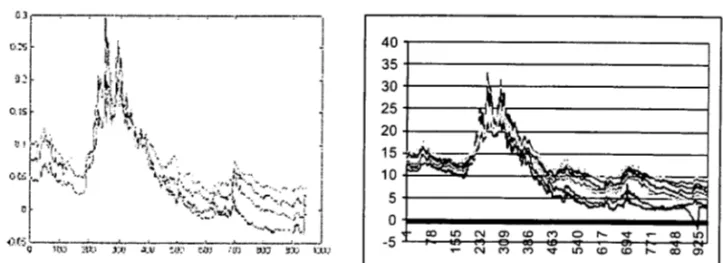
20 years in contrast to 3 in Brazil. Figure 5 shows the trajectory of those rates.
They display less correlation than in Brazil. The first component explains only 85%
of the total variation, which suggests a limitation of having only 1 factor.
o
o
o
o
o
o
o
o
o
o
o
o
o
o
o
o
o
o
o
o
o
o
o
o
o
o
o
o
o
o
o
o
o
o
o
o
o
o
o
o
o
o
o
o
o
o
o
o
The estimated LL was (-3866) and the IMM was nil, indicating that in this case
multiple modes case were not found. The table C1 shows that the parameters were
estimated with precision.
Tab C-1:Risk Premium
ÀD À. <I> Il V
A
1JI 1.0932 -0.2298 0.7533 0.0031 0.0018
SD 0.0029 0.0002 0.011
o
o
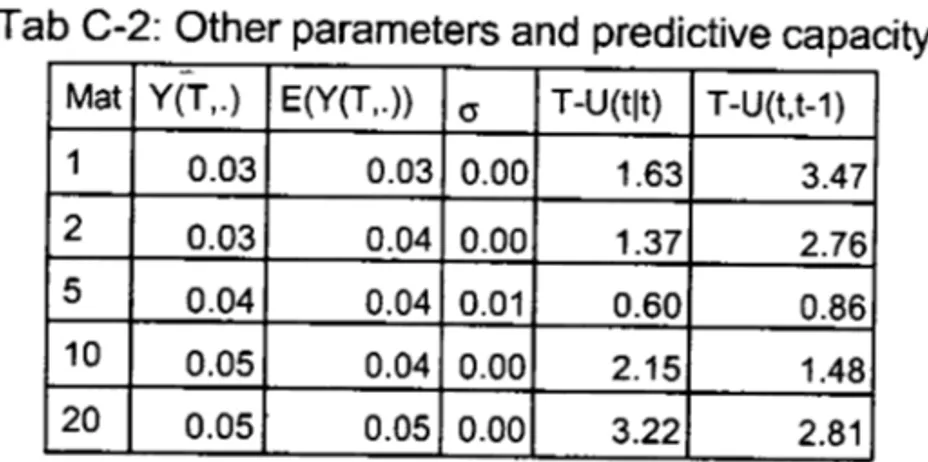
Table C2 shows that the term structure in the last period - may of 2005 - is
predicted similarly to the observed, but that the predictive capacity of the model is
inferior to the random walk except for the maturity of 5 years. This is further
evidence of the limitations of a model that has only one factor to explain the
movements of the term structure. To evaluate if the monthly specification with lags
of 21 days could be the source of the low predictive mpacity, the model was
estimated in a daily specification, and that type of result was maintained.
Therefore, the inclusion of information contained in a second latent factor could be
important to strengthen the predictive capacity in a case were one has bnger
maturities.
Tab C-2: Other parameters and predictive capacity
-Mat Y(T,.) E(Y(T,.)) cr T-U(tlt) T-U(t,t-1)
1 0.03 0.03 0.00 1.63 3.47
2 0.03 0.04 0.00 1.37 2.76
5 0.04 0.04 0.01 0.60 0.86
10 0.05 0.04 0.00 2.15 1.48
20 0.05 0.05 0.00 3.22 2.81
The figure 5 shows that, according to the model, in USA the monetary shock is
Fig5: IRF and Trajectory of American Rates of a number of maturities
0.2 - r - - - . - - - ,
o
1 2 3 4 5 6 7 8 9 10
....---...,
- r O
- r 1
0 " _ 0 r2
- r 5
- r 1 0
- r 2 0
Ü(1f i
()"~~
.
~
::~~~~~i::~:;~;~:~;:~~::~f~~
j
OQl
~~
, '.;',
lo". •.~
',"" : J"'v-(1(,; I':.;::.<.~:~,/,.~
....
:~:/ ~!J _~ _J _ _ J. _~ Jo _____ J_. ~~ .. _ _ _ _ _ _ _ ;t _ _ ~. ____ • _ _ _ _ :
iJ '0) :~1j 'ff..1 't(1 :((1 «ú iL'Ú ~JJ (~:(, 1(\))
3.5 Case D: Sovereign Spread and shocks over its determinants
This is the last case, and one of the objectives of this article is to utilize AP's
framework in the credit risk setting. This model relates the dynamics and the risk
premiums of the Brazilian sovereign spreads to the dynamics and the risk
premiums of American rates, and includes' the effect of a measure of the
vulnerability of the Brazilian public debt. Unfortunately this version can be subject
to some criticisms beforehand, due to empiricallimitations.
Up to the knowledge of the authors, there do not exist available measures of the
spread or of the interest rates of the externai bonds issued by the Republic of
Brazil corrected to constant maturity, The obligations are issued with coupon
payments. For this reason, we utilized a methodology described briefly in the
appendix to calculate the Zero-Coupon curve. The prices of the bonds were
obtained from the Morgan Market, which do not dispose of bonds with short
maturities already matured, This turned the estimation of the spreads especially
precarious in the beginning of the sample. Figure 6 in the following shows the rates
of return of selected bonds and the constant maturity spread rates.
O
O
O
O
O
O
O
O
O
O
O
O
O
O
O
O
O
O
O
O
O
O
O
O
O
O
O
O
O
O
O
O
O
O
O
O
o
;0
O
,o
,O
'0
iO
O
lO
10
:0
'O
10
lo
O
O
O
O
O
O
O
O
O
O
O
O
O
O
O
O
O
O
O
O
O
O
O
O
O
O
O
O
O
O
O
O
O
O
O
Fig 6: Constant maturity spreads and rates of the bonds.
4 0 , - - - ,
35+---~
30 \
25 " 11
2 0 .
~~~;.'t
,.,-!.~---15~.~ ..
10 IJS' ~"'!!'!'l 'Af\,~ . ._ ... _.-=
5 ~"~~J....~
o~---·~---~~,r
-5 .L.-...jCX)~LO~N~a>~tOi___<fi(")~o-/'.:._.._...V~ ... ____'CX)i_NJLO
~ N M M ~ ~ ~ ~ ~ ~ ~
The spreads of those bonds are negotiated outside of Brazil and are related to the
risk of default. Thus, it is convenient to incorporate a measure of vulnerability of the
indebtedness of the country or of the Brazilian state. Since in most part of the
sample period - 2001/2005 - the majority of the Brazilian public debt was
indexed to a foreign currency, as bonds issued abroad or as bonds issued in the
domestic market but indexed to the exchange rate, the exchange rate is a synthetic
and diary exposition to risk. Unfortunately for our objectives, but fortunately for our
country, the government adopted the policy of reducing drastically the debt indexed
to the US$, which turned this measure improper towards the final ofthe sample.
In this model, the state variables X are the short rate (r) in USA, the log of the real
exchange rate (c), and the short credit spread of Brazil (s) - that due to lack of
information was the spread relative to 1 year. The model was estimated
conditional to the risk premium and the dynamic properties of the rates in USA
estimated in the previous case.
The stochastic process of the state variables and the risk premium are:
The estimated model found LL=-2015 and IMM=272, which indicates that the
algorithm found multi pie modes, ànd that there are expressive differences among
that for some of the estimators one does not reject the hypothesis that they are
null, suggestin!~, as in case B, the existence of identification problems.
Tab 0-1 : Risk Premium
c) À.Ü(s) À(c,r) À(c,c) À(c,s) À(s,r) A(s,c) À(s,s)
0.93 1.51 0.48 1.86 -0.70 -0.04 0.07 0.73
0.107 0.068 0.808 0.001 0.003 0.103 0.001 0.004
This model does not exhibit predictive capacity. Also, the term structure is not
adequately predicted.
Tab 0-2 : Other statistics
Mat T-U(tlt). T-U(tlt-1 ) cr E(Y(T,.)) Y(T,.)
6 7.11 6.93 0.07 0.06 0.01
10 6.24 6.09 0.05 0.06 0.02
20 11.56 11.36 0.04 0.07 0.03
The structural shocks of the model were identified supposing that the shocks of
interest rates in USA are exogenous for the Brazilian economy, and that the
shocks in the vulnerability - the exchange rate - are determined by the
externai shocks and determines the unexpected alterations of the spread. This
order defines how was defined the Cholesky decomposition used to identifie
these structural schoks in the Var model. Those shocks were denominated as
externai (R), vulnerability (C), and spread (S).
The figures below show the dynamic properties of this model:
• The effects of the shocks over the spread are: The increase of the
vulnerability has a short and transitory positive effect; the rise of the
perception of risk has a positive effect for a longer period; and, finally,
the externai shock has an increasing effect over the spread.
• Only the variance decomposition of the effect of the spread of maturity
20 is shown, because the other maturities are similar. In the tenth month
after the shock, the effect of the shock explains 40% of the variation,
whereas the vulnerability shock has no effect anymore and the spread
shock explains the complement.
O
O
O
O
O
O
O
O
O
O
O
O
O
O
O
O
O
O
O
O
O
O
O
O
O
O
O
O
O
O
O
O
O
O
O
O
O
o
o
o
o
o
o
o
o
o
o
o
o
o
o
o
o
o
o
o
o
o
o
o
o
o
o
o
o
o
o
o
o
o
o
o
o
o
o
o
o
o
o
o
o
o
o
o
o
Fig7: IRF ofthe Real Exchange Rate and ofthe Spreads to Shocks
2.50 2.00 1.50 1.00 0.50 0.00 -0.50 -1.00 ... ~ [:;-~_ .. •... , .. _-.,.-.. ...
--=====-===
~-
~ ,~ 2.502.00 ",
a
1.50[3
=~
1.000.50
0.00
-0.50
Fig9:IRF and VDF: Externai Shock (US short rate shock)
0.12 . . . - - - ,
0.1 ~"'---_;
0.08
+-->.",,,---1
I
s'l
O.OS ~~";:,,,.,"'_....,.---l0.04\. " ' - - - -
~
=~~
O.O~ t--'.~~-.,.=.=.-
.. -: ... -:-:-=.== ...::.=;:::8
-0.02 ... .., " " ' .. ,, n . "
"'-:.. ..
0.8
-...~
~
O.S +----"--::=::---=---i - S20
0.4 - S " S
0.2 --····S10
o
--0.2 1 ? ':! fi " " 7 A a 1 f'I
Fig10:IRF and VDF : Vulnerability shock (real exchange rate)
0 . 0 8 . . . - - - ,
O.OS
0.04 +---"'-..,::---!
- S 1 0
8
"
S-'-..
0.02 +-=::;;:::",,~---=:::-..,~:::-.--; ____ S20
o+-~~~~~~~~
..L.. 1~2~3_4~5~S~7~8~9~1~0
-0.02
Fig11 :IRF and VDF: Spread shocks
O.OS . , . . . . - - - , 0.04 ~---_~--.--- =., =:-1 0.02 ~.
o ----
./.--/ ./.--/
-0.02 .. /" v v
-0.04 ; -O.OS /
-0.08 - r ' - - - I
-0.1 - ' - - - '
1 . 2 . , . . . . - - - ,
1 +---/'7' ~ .. , . - - - l
a
0.8 +-~/;'---"_,;_.,-. - - - - i - S"S
O.S - S 1 0
/
1 2 3 4 5 S 7 8 9 10
4.Conclusion
This exercise showed the variety of questions that a simplified version of the AP's
model is able to treat, tle effect of this simplification over the predictive capacity of
the longe r rates, and the difficulties of the estimation of risk premiums even in this
simplified setting. Those difficulties suggest the existence of limitations concerning
the possibility á estimating ali the parameters of risk premium, and therefore the
necessity of investigating how to introduce restrictions over the specifications of the
risk premium in order to make them identifiable to the models with more than one
factor.
We proposed a simplification and a method of estimation that to our point of view
greatly reduced identification problems, but we recognize that using the short rate
as the only latent variable constrained the predictive and explanatory capabilities of
our model.
On the other hand, we believe that the addition of a new state variable, namely the
short spread, alleviated that problem when studying the Brazilian sovereign curve.
More importantly, a major objective of our line of research is trying to find the
determinants of the credit spreads, since the understanding of the credit spread is
of utmost impOlrtance in the study of emerging markets term structure, and a model
with more latent variables would make the estimation process too complex.
Furthermore, our proposal is a multidimensional affine,model for the term structure
of interest rates: that is as easy to estimate as common empirical procedures.
In view of empirical difficulties due to lack of data, our results are still preliminary,
but we document that exchange rate and the American short rate explain a
significant portion of the Brazilian term structure. Moreover, it must be stressed that
only difficulties with lack of data prevent us of studying the relation of more
macroeconomic variables with the interest rates and credit spreads.
Our results up to this point shows interesting interactions between financiai and
macro variables. For instance, in the model B the effect of exchange rate shocks
explains a major part of the variation of interest rates, and the effect grows with
O
O
O
O
O
O
O
O
O
O
O
O
O
O
O
O
O
O
O
O
O
O
O
O
o
o
o
o
o
o
o
o
o
o
o
o
o
o
o
o
o
o
o
o
o
o
o
o
o
o
o
o
o
o
o
o
o
o
o
o
o
o
o
o
o
o
o
o
o
o
o
o
longer maturities, and in the model D the externai shock has an increasing effect
over the spread.
Future work will also contemplate the correlation effects among the emerging
countries. That is, we would like to know for instance how Brazilian credit spread is
affected or affects Russian or Argentinean credit spread. This kind of study can be
more easily implemented in the present setting than in continuous time models.
Moreover, the addition of correlation will enable us to have 3 latent variables as
state variables, namely, the risk-free short rate, and the Brazilian and, for instance,
the Russian short spreads, and studies by Litterman and Scheinkman and Dai and
Singleton have indicated that exactly 3 state variables are need to study 1I1e term
structure.
Finally, we list tasks to be immediately executed:
• To Obtain a more accurate description of the term structure of the spreads, in
particular a more adequate measure of the short rate;
• To Search for another measure of the vulnerability of the indebtedness,
eventually measured monthly or trimester;
• To Extend the model to consider more than one quantitative fa cto r
References:
1. A no-arbitrage vector autoregression of term structure dynamics with
macroeconomic and latent variables, 2003, Ang A. Piazzesi, M. Joumalof Monetary Economics 50,745-787.
2. No-Arbitrage Taylor Rules, 2005, Ang, Andrew; Oong, Sen and Piazzesi,
Monika. Working pape r, University of Chicago.
3. Modeling Bond Yields in Finance and Macroeconomics, Francis X. Oiebold,
Monika Piazzesi, and Glenn O. Rudebusch, American Economic Review P&P
(2005)
4. Ouffie, O., Kan, R., 1996. A Yield-Factor Model of Interest Rates, Mathematical
Finance, 6, 379-406.
5. Harrison, J. M., Kreps, O. M., 1979. Martingales and Arbitrage in Multiperiod
Securities Markets, Journal of Economic Theory, 2,381-408.
6. Chen, R. R, Scott, L., 1993. Maximum Likelihood Estimation for a Multi-factor
Equilibrium Model of the Term Structure of Interest Rates, Journal of Fixed
Income, 3, '14-31.
7. Ouffie, O., l.. Pedersen, and K. Singleton (2000). Modeling Sovereign Yield Spreads: A Case Study of Russian Oebt, Journal of Finance 58,119-159.
8. Ouffie, O. and K. Singleton (1999). Modeling Term Structures of Oefaultable
Bonds, Review of Financiai Studies 12,687-720.
9. Litterman, R, Scheinkman, JJ1991) Common factors affecting bond returns,
Journal Fixed Income, 1, 51-61
10. Dai,
a.,
Singleton, K. (2000),Specification Analysis of term structure of interest rates, Journal of Finance 55,1943-78.O
O
O
O
O
O
O
O
O
O
O
O
O
O
O
O
O
O
O
O
O
O
O
O
O
:0
:0
O
O
:0
:0
iO
O
O
O
O
O
Q
O
O
Q
Q
O
O
O
O
O
O
O
O
O
O
O
O
O
O
O
O
O
O
O
O
O
O
O
O
Q
O
O
O
O
O
O
Appendix : A 1 - Constant Maturity Interested Rate Calculation
The price of bond i with coupon (x), maturity (T), yield to maturity O) is: P(t,i) = (1 +j(i))-T(i)-t + ~T(i) xCi)
~k=t (1 + } ( i ) / - t
The same price can be calculated using the term structure r(k)
P(t,i) = (1+r(T(i)))-T(i)-t + ~T(i) xci)
~k=t (1 + r(k»k-t
Supposing bonds are ordered by the maturities T(1 )<T(2)< ..
For k=1 : r(i)=j(1) 'Vi<=T(1)
P(t i) = ~ T(i-I) xci) +( 1 +rr T(i)-t + ~ T(i) x( i)
, ~k=t (1 + r(k»k-t ~k=T(i-1)+1 (1 + r)k-t
For T(i-1) < k <= T(i), r(k)=r_(i )
P(t i) = ~2T(i-1) x(i)/2 +(1+r)-(T(i)-t) + ~2T(i) x(i)/2 or
, ~k=flooI{2t)+1 (1
+
r(k»k!2-t ~k=2T(i-I)+1 (1+
r/l2-t 'P* = ZT(i)-t + xCi) ~T(i). zk-t = ZT(i)+1-t[ xci) (1-zn+1)/(1-z)+ zn]
~k=T(I-I)+1
where
P* = P(t,i) _ ~T(i-I) xCi)
~k=t (1
+
r(k»k-tz = (1 +r)-1
the term rate for the interval T(i), T(i+1) is given by the maximum real positive root
of ZT(i)+1-t (x(i)+1) - ZT(i)-t -ZT(~1)+1-t xCi) - P*(z-1)
=
OA2. Bonds used to calculated the spread : Brazilian Sovereign Bonds
BR Republic 9 5/8% due 05 Yld To Mal BR Republic 77/8% due 15 Yld To Mat
BR Republic 10 1/4% due 06 Yld To Mat BR RepUblic 11 % due 17 ITL Yld To Mat
iBR Republic 11 1/4% due 07 Yld To Mat BR Republic 8 7/8% due 19 Yld To Mat
IBR Republic 10% due 07 GBP Yld To Mat BR Republic 12 3/4% due 20 Yld To Mat
iBR Republic 9.3/8% due .08 Yld To Mat BR Republic 8 7/8% due 24 Yld To Mat
aR Republic 141i2% due_09 Yld To Mat BR Republic 8 7/8% due 24- B Yld To Mat
.-IBR Republic 91/4% due 10 Yld To Mat BR Republic 83/4% due 25 Yld To Mat
IBR Republic 12% due-10 Yld To Mat BR Republic 101/8% due 27 Yld To Mat
IBR Republic 10% due 11 Yld To Mat BR Republic 121/4% due 30 Yld To Mat
IBR Republic 11 % due 12 Yld To Mat BR Republic 81/4% due 34 Yld To Mat
IBR Republic 101/4% due 13 Yld To Mat BR Republic 11 % due 40 Yld To Mat
FUNDAÇÃO GETULIO VARGAS
BIBLIOTECA
ESTE VOLUME DEVE SER DEVOLVIDO A BIBLIOTECA NA ÚLTIMA DATA MARCADA
I
I:
BIBLIOTECA
--MARIO HENRIQUE SIMONSEN FUNDAÇÃO GETÚLIO VARGAS
~10«33
O
O
O
O
\)O
O
O
O
O
O
O
O
O
O
O
O
O
O
O
O
Q
O
O
O
O
O
O
O
O
O
O
O
O
Q