ESCOLA DE P ´
OS-GRADUA ¸
C ˜
AO EM
ECONOMIA
Raphael de Albuquerque Galv˜
ao
Optimal regulation of oil fields under asymmetric
information
Optimal regulation of oil fields under asymmetric
information
Disserta¸c˜ao submetida `a Escola de P´ os-Gradua¸c˜ao em Economia como requesito par-cial para a obten¸c˜ao do grau de Mestre em Economia.
´
Area de Concentra¸c˜ao: Economia
Orientador: Humberto Luiz Ata´ıde Moreira
Neste trabalho ´e analisada a rela¸c˜ao entre um regulador e uma empresa petrol´ıfera. H´a v´arias incertezas inerentes `a essa rela¸c˜ao e o trabalho se concentra nos efeitos da assimetria de informa¸c˜ao. Fazemos a caracteriza¸c˜ao da regula¸c˜ao ´otima sob infor-ma¸c˜ao assim´etrica, quando o regulador deve desenhar um mecanismo que induz a firma a revelar corretamente sua informa¸c˜ao privada. No caso em que a firma n˜ao pode se comprometer a n˜ao romper o acordo, mostramos que o regulador pode n˜ao implementar o resultado ´otimo que ´e obtido sob informa¸c˜ao completa. Nesse caso, o regulador n˜ao consegue compartilhar os riscos com a firma de forma ´otima. Por fim, ´e apresentado um exemplo, em que mostramos que a condi¸c˜ao de Spence-Mirrlees (SMC) pode n˜ao valer. Esse resultado aparece de forma natural no modelo.
This work considers a relationship between a regulator and an oil company. There are many uncertainties inherent in this relationship and we focus on the effects of asymmetric information. We characterize the optimal regulation under asymmetric information, when the regulator must design a mechanism that induces truthful revelation about the firm’s private information. We show that, when the firm cannot commit not to quit the relationship, the regulator may not be able to implement the optimal first-best regulatory outcome. In this case, the regulator cannot achieve the optimal risk-sharing with the firm. We also provide an example, in which we show that the Spence-Mirrlees condition (SMC) may not hold. As it turs out, this is a natural result in our model rather than an imposition.
1 Introduction 1
2 The model 4
2.1 First-best . . . 7
2.1.1 No ex post IR constraint . . . 8
2.1.2 Ex post IR constraint. . . 9
3 Asymmetric information 11 3.1 Ex post IR constraint . . . 12
3.1.1 Private information about β . . . 12
3.1.2 Private information about θ . . . 14
3.1.3 Private information about β and θ . . . 16
3.2 No ex post IR constraint . . . 19
3.3 Positive reservation utility . . . 20
3.4 Results . . . 22
4 An example 24 4.1 Numerical results . . . 24
4.1.1 Effort . . . 25
4.1.2 Investment. . . 25
4.1.3 Welfare . . . 26
4.2 Violating the Spence-Mirrlees condition . . . 27
5 Conclusions 29
References 30
1
Introduction
In this work we use contract theory to characterize the optimal regulation in the oil industry. There are many uncertainties inherent in petroleum contracts and our goal is to analyze the effects of asymmetric information in the relationship between a regulator and an oil company. In general, the company has superior information about the charac-teristics of a certain area to be explored and, once a discovery is made, the company has more information about its efficiency in oil extraction. Thus, the regulator must provide incentives for the company to reveal its private information.
Our work is based on the regulation model with investment in Laffont and Tirole
(1993) and in Aghion and Quesada (2010). The former is a classical regulation model under asymmetric information, and the latter is a work applied to the oil industry.
Aghion and Quesada (2010) use contract theory to analyze potential sources of inefficiencies in petroleum contracts signed between two parties: the government and an oil company. They develop a simple model of exploration and production, in which there is sunk investment in exploration and, conditional on discovery, extraction requires a noncontractible effort. The model addresses uncertainties inherent in petroleum contracts and, in light of recent events, the main concern is to understand why governments may renege on past agreements with oil companies on the grounds that those agreements were unfair.
Investments are risky because the existence, size, and quality of the reserve are uncertain, and the drilling costs are very difficult to anticipate. In most countries, gov-ernment owns natural resources under the surface, hence a new goverment may force contract renegotiations. Aghion and Quesada (2010) also say that sunk investments in oil exploration are large and very specific in nature and, therefore, if the oil company is in charge of the investment, it is subject to opportunistic behavior and holdup when a discovery is made. After production begins, the government may increase taxes or even expropriate the firm to increase its take. The company takes into account that possibility and underinvests.
In our model, we eliminate some of the sources of contractual inefficiency addressed in Aghion and Quesada (2010). We assume that contracts are always enforced and, in our framework, the government does not have the possibility to adopt an opportunistic behavior, since there is full commitment. Furthermore, we do not analyze the existing contract forms, which is done in their work. However, we consider additional sources of inefficiency, focusing on the effects of asymmetric information on petroleum contracts. We take some important features of Aghion and Quesada (2010) and adapt their model to the framework in Laffont and Tirole(1993).
Laffont and Tirole (1993) develop a simple regulation model in which an individual public project has a fixed value for consumers. A regulator hires a firm to realize the project and, if the firm exerts effort, it decreases the cost of the project. The firm can be more or less efficient in cost reduction and, since the effort is not observable for the regulator and it is costly to the firm, the moral hazard problem arises when the firm’s efficiency parameter is private information. In this case, the regulator must offer a direct mechanism to the firm that induces truthful revelation. The mechanism specifies a level of cost for the project and determines a net monetary transfer to the firm.
Laffont and Tirole (1993) also introduce an investment stage to the problem. In this extension, the firm can realize a sunk investment that determines the probability distribution for the firm’s efficiency parameter in the production stage. There may be a parameter of effectiveness of investment and the authors analyze the case where the firm has superior information about this parameter.
We develop a regulation model with two parties, the regulator and a firm. There are two periods, an exploration stage, when the firm realizes a sunk investment, and, conditional on discovery, there is a production stage, when oil is extracted by the firm. We assume that there may be asymmetric information in both periods: either the firm’s efficiency in extraction or the effectiveness of the investment in exploration can be private information to the firm. Hence, the regulator must design a mechanism to induce truthful revelation about the firm’s private information. We assume that the regulator’s objective is to maximize the social welfare.
the level of production cost contracted for the second period is a function of the sunk investment, realized in the first period, and its effectiveness parameter.
We also provide an example with numerical results. In the example we show that the Spence-Mirrlees condition (SMC) may not hold. The SMC has been the main assumption that allows the characterization of the solution of one-dimensional adverse selection or hidden information models. It turns out that this condition can be violated in a very natural way in our model.
2
The model
We develop a model of regulation under asymmetric information that reflects some uncertainties inherent in the oil industry. In our model, the regulator hires a risk neutral oil company to work in a project that, if successful, has a fixed payoff. The firm is responsible for exploration and production. FollowingAghion and Quesada (2010), there is one exploration period (T = 0), when the firm makes a sunk investment I, and one production period (T = 1).1 As in their model, the regulator offers a contract to the
firm in (T = 0) and, after it is accepted, exploration begins. Unlike Aghion and Quesada
(2010), we assume that contracts are enforceable and that there is full commitment, so that the regulator cannot change any rules after the contract is signed.
Our model is based on the regulation model with investment in Laffont and Tirole
(1993). We assume that production costs and investment are observable variables for the regulator, but there may be asymmetric information about the effectiveness of the investment and about the firm’s efficiency in reducing production costs. As inLaffont and Tirole(1993), we take the accounting convention that the production and investment costs are reimbursed to the firm by the regulator and we assume that the firm is compensated by a net monetary transfert to work for the regulator.
Let the effectiveness of investment be measured byβ ∈[β,β¯]≡B, known by the firm at the beginning of period (T = 0). This parameter can represent geological uncertainties in the area to be explored. For a given pair (β, I), an oil reserve is discovered with probability Q(I, β) >0, increasing and concave in I and in β, with limI→∞Q(I,β¯) ≤1,
and we make the following assumption:2
Assumption 1 QβI >0.
Whenβis private information to the firm,G(·) is the absolutely continuous function, with densityg(·), that describes the prior of the regulator on the interval [β,β¯]. We assume that g(β)>0, for allβ ∈B.
The setting in period (T = 1) is similar to Laffont and Tirole (1993). Conditional on discovery, there is an expected production of 1 unit of petroleum in period (T = 1). The production is sold at a pricepand the revenue goes to the regulator. The production cost function is
c=θ−e (1)
whereθ ∈[θ,θ¯]≡Θ is an efficiency parameter, which the firm learns at the beginning of
1
Their general model considers two exploration periods.
2
(T = 1), andeis the manager’s noncontractible effort, which costsψ(e) monetary units to the firm. Functionψ is increasing and convex, with ψ(0) = 0. The absolutely continuous cumulative distribution ofθ is denoted by F(·), with densityf(·)>0.
The main difference between our model andLaffont and Tirole(1993) is that, instead of affecting the distribution of θ, investment and its effectiveness parameter β partially determine the project’s probability of success. Unlike Aghion and Quesada (2010), the cost of effort in our model is not affected by the sunk investment, and the effort does not increase expected production. However, the effort in our model reduces production costs and therefore increases the net expected revenue of the project. Another difference from
Aghion and Quesada(2010) is that they do not consider multiple types in the exploration period or in the production period. In their model, investment completely determines the probability of discovery and there is no parameter of efficiency in cost reduction.
We assume that the regulator’s objective is to maximize the expected social welfare in period (T = 0). As in Laffont and Tirole (1993), the regulator is a Stackelberg leader and makes a take-it-or-leave-it offer to the firm in period (T = 0). The regulator offers a contract (I(β), t0(β), c(θ, β), t1(θ, β))
θ∈Θ for each type β, based on the observables t, c
andI. The contract specifies: a level of investmentI(β) and a net monetary tranfert0(β)
in (T = 0); a production costc(θ, β) for each possible parameterθ in (T = 1) (conditional on discovery); a net transfer t1(θ, β) for each θ the regulator may observe in (T = 1)
(conditional on discovery). We consider a more general set of contracts thanLaffont and Tirole(1993). In their model, the regulator can only give monetary transfers to the firm in the production period, while we consider another transfer in the the investment stage.
For a given pair (θ, β), the firm’s ex post level of utility in period (T = 1) is
U(θ, β) =t1(θ, β)−ψ(e(θ, β)) (2)
and, given β, the firm’s ex ante expected utility when it signs the contract in period (T = 0) is
U(β) = Q(I(β), β)Eθ[U(θ, β)] +t0(β). (3)
whereEθ[x] = Rθ¯
θ[x]f(θ)dθ.
When the firm accepts the contract in (T = 0), the expected utility U is known, but the ex post utility in period (T = 1) is not, since it depends on success in exploration and, if oil is discovered, it is a function of the firm’sθ, which is learned in (T = 1).
the regulator as outside the relationship. The firm’s reservation utility (the level of utility it obtains if the contract is not signed), is normalized to 0, which leads to the firm’s individual rationality (IR) constraint
U(β)≥0. (IRex ante)
In the production period (T = 1), if the firm does not work for the regulator its utility is also 0. Thus, the firm’s ex post IR constraint is
U(θ, β)≥0. (IRex post)
and we consider two possibilities:
i. the firm can commit to produce even if the contract ex post results in a level of utility below its reservation utility in (T = 1);
ii. the firm cannot commit to produce in period (T = 1) if it results in a level of utility below its reservation utility.
In (ii) above, welfare maximization must be subject to the ex post IR constraint.
As in Laffont and Tirole (1993), let λ > 0 be the shadow cost of public funds. It means that distortionary taxation inflicts a disutility of 1+λmonetary units on taxpayers for every monetary unit that goes to the state. Hence, given θ and β, the aggregate net surplus in period (T = 1) is
p−(1 +λ)[c(θ, β) +t1(θ, β)] +U(θ, β)
which can be written as
p−(1 +λ)[θ−e(θ, β) +ψ(e(θ, β))]−λU(θ, β).
W(β) = Q(I(β), β)Eθ[p−(1 +λ) (θ−e(θ, β) +ψ(e(θ, β)))−λU(θ, β)]
−(1 +λ)I(β)−λt0(θ, β)
which is equivalent to
W(β) =Q(I(β), β)Eθ[p−(1 +λ)(θ−e(θ, β) +ψ(e(θ, β)))]−(1 +λ)I−λU(β). (4)
The first term in (4) is the expected net revenue of the project (the difference between the payoffpand the total costc+ψ(e), as perceived by the taxpayers, times the probability of success Q). The social welfare is the difference between this expected revenue and the investment cost in (T = 0) (as perceived by the taxpayers) plus the firm’s rent above its reservation utility times the shadow cost of public funds. Although the project’s payoff and the firm’s utility are equally weighted in the welfare function (4), leaving rent to the firm reduces social welfare in the existence of a shadow cost λ >0.
2.1
First-best
We first analyze the model under complete information to establish benchmark first-best levels of effort and investment and the first-first-best level of social welfare. The regulatory outcome in this section results in the highest level of social welfare the regulator can achieve. In this case, besides the cost c and the investment level I, parameters β and
θ are also observable variables for the regulator. For a given β in period (T = 0), the regulator solves
max
I(·),e(·),U(·)Q(I(β), β)Eθ[p−(1 +λ)(θ−e(θ, β) +ψ(e(θ, β)))]
−(1 +λ)I(β)−λU(β)
subject to an individual rationality constraint, wheree(θ, β) =θ−c(θ, β).
2.1.1 No ex post IR constraint
For a given β in period (T = 0), the welfare maximization problem is
max
I(·),e(·),U(·)Q(I(β), β)Eθ[p−(1 +λ) (θ−e(θ, β) +ψ(e(θ, β)))]
−(1 +λ)I(β)−λU(β)
subject to the ex ante IR constraint
U(β)≥0. (IRex ante)
The characterization to this program is in the Appendix. The optimal effort solves
ψ′
(e(θ, β)) = 1 (5)
or
e(θ, β) = ψ′−1(1) ≡e∗ ,
the optimal first-best level of investmentI∗
(β) is the solution to
QI(I ∗
(β), β)(p−(1 +λ)(E[θ]−e∗
+ψ(e∗
))) = 1 +λ (6)
and the regulator sets
U(β) = 0. (7)
This outcome can be implemented in many different ways. In particular, the regu-lator can set t1(θ, β) = ψ(e∗
) and t0(β) = 0, so that the ex post IR constraint is always
satisfied3.
Condition (5) implies that marginal disutility of effort, ψ′
(e), must be equal to the marginal production cost reduction, which is 1. Condition (6) implies that the marginal cost of investment (as perceived by the taxpayers), 1 +λ, must be equal to the expected marginal net revenue of the project. Furthermore, since rents are socially costly, the
3
To satisfy the ex post IR constraint and to give the firm the utilityU(β) = 0, the regulator can set
t1
(θ, β) =ψ(e∗) +a(β) andt0
regulator leaves no rent to the firm, i.e., condition (7) holds.
2.1.2 Ex post IR constraint
We now assume that the firm cannot commit to produde if, given the realization of
θ, the contract results in negative utility in period (T = 1). The firm’s utility in period (T = 1) as a function of its true parameters β and θ is U(θ, β) = t1(θ, β)−ψ(e(θ, β)),
and the ex post IR constraint is
U(θ, β)≥0. (IRex post)
In this case, for a given β in period (T = 0), the welfare maximization problem is
max
I(·),e(·),U(·),t0(·)Q(I(β), β)Eθ[p−(1 +λ)(θ−e(θ, β) +ψ(e(θ, β)))−λU(θ, β)] −(1 +λ)I(β)−λt0(β)
subject to (IRex ante) and (IRex post).
The solution to this program is
e(θ, β) =e∗
I(β) =I∗
(β)
U(θ, β) = 0
t0(β) = 0
which implies thatU(β) = 0, i.e., no rent is left to the firm.
Thus, the optimal regulatory outcome if we consider ex ante or ex post IR constraints is the same. As noted before, the solution to the this program is a particular solution of the welfare maximization problem when it is not subject to the ex post IR constraint.
We summarize our results in the next proposition.
Proposition 1 Optimal regulation under complete information is characterized by (5), (6), and (7).
i. an increasing level of investment in β;
ii. a constant level of effort and increasing costs in θ;
iii. no rent for the firm.
For each pair of parameters (β, θ), the pair (I∗
(β), e∗
3
Asymmetric information
In this section we add asymmetric information to the model. As discussed before, the firm may not be able to commit to produce if the contract ex post results in a level of utility below its reservation utility level in (T = 1). Therefore, we consider that the maximization problem may be subject either to ex ante or to ex post individual rationality (IR) constraints. In each setting we analyze three different cases:
• Case (β): β is private information to the firm and θ is common knowledge;
• Case (θ): β is common knowledge and θ is private information to the firm;
• Case (θ, β): both parameters are private information to the firm.
If any parameter is not observable by the regulator, a direct mechanism that induces truthful revelation must be offered to the firm. Thus, the regulator offers a direct mecha-nism I( ˆβ), t0( ˆβ), c(ˆθ,βˆ), t1(ˆθ,βˆ)
(ˆθ,βˆ)∈Θ×B. If the firm accepts the mechanism, it makes
an announcement ˆβ of its parameter in period (T = 0), then it realizes an investmentI( ˆβ) and receives a net monetary tranfer t0( ˆβ). Conditional on discovery, the firm announces
ˆ
θ in period (T = 1) and produces at a costc(ˆθ,βˆ), receiving a net transfer t1(ˆθ,βˆ). From
the Revelation Principle, there is no loss of generality in restricting the regulator to direct and truthful mechanisms.
The regulator’s optimization problem must be subject to the incentive compatibility (IC) constraints, which ensure that the firm truthfully reveals its type. Let the firm’s true parameter in (T = 0) be β and suppose that the efficiency parameter in the production period is θ and the announced one is ˆθ. The firm’s utility in (T = 1) is
ϕ(θ,θ, βˆ )≡t1(ˆθ, β)−ψ(θ−c(ˆθ, β)) (8)
and the utility conditional on truth-telling is
U(θ, β) =ϕ(θ, θ, β). (9)
Thus, for each pair (β, θ), the IC constrains are
θ ∈ argmax
ˆ θ∈Θ
ϕ(θ,θ, βˆ ) (IC1)
and
β ∈ argmax
ˆ β∈B
We say that a contract is implementable if it satisfies the IR and IC constraints.
Our goal is to characterize the optimal regulatory mechanism under asymmetric information and to analyze the trade-off between incentives and rent extraction. The regulator must provide incentives for truth-telling about the firm’s parameters, but giving rent to the firm is socially costly. Furthermore, we want to analyze the incentives schemes used by the regulator when each parameter is private information, and how is the inter-action between incentive provision in the exploration period and in the production period when there is asymmetric information in both periods. We compare the social welfare in each case with the benchmark first-best level of welfare.
3.1
Ex post IR constraint
We first characterize the optimal regulatory outcome when the firm cannot commit to produce if its ex post utility is lower than its reservation utility level for a bad realization of θ in period (T = 1).
3.1.1 Private information about β
Suppose that the efficiency parameter θ is common knowledge in period (T = 1), but parameter β is private information to the firm in period (T = 0). In this case, the regulator offers a mechanism I( ˆβ), t0( ˆβ), c(θ,βˆ), t1(θ,βˆ)
(θ,βˆ)∈Θ×B in (T = 0). The
mechanism determines a level of investment and a monetary transfer t0 in (T = 0) for
each announcement ˆβ the firm makes about its parameter, and for each ˆβ and each true paramenterθ the regulator may observe in (T = 1), it specifies a level of production cost and a net transfert1.
Let the firm be ex ante type β. The firm’s expected utility is given by
U(β) = sup
ˆ β∈B
Q(I( ˆβ), β)Eθ[U(θ,βˆ)] +t0( ˆβ). (10)
The regulator’s maximization problem is now subject to the ex post IR and the IC constraint for β. Hence, the regulator solves
max
I(·),e(·),U(·),t0(·)
Z β¯
β
Q(I(β), β)Eθ
p−(1 +λ)[θ−e(θ, β) +ψ(e(θ, β))]
−λU(θ, β)
−(1 +λ)I(β)−λt0(β)
subject to
β ∈ argmax
ˆ β∈B
Q(I( ˆβ), β)Eθ[U(θ,βˆ)] +t0( ˆβ). (IC0)
U(β)≥0 (IRex ante)
and
U(θ, β)≥0. (IRex post)
It is straightforward to see that the first-best regulatory outcome can be achieved and therefore it is the solution to this program. The regulator can implement the first-best level of effort e∗
and sett1(θ, β) =ψ(e∗
), so that the firm has a fixed ex post utility
U(θ, β) = 0. In this case, we prove in the Appendix that the sufficient conditions for IC in period (T = 0) are
˙
U(β) = Qβ(I(β), β)Eθ[U(θ, β)] (IC0.a)
and
˙
I(β)≥0. (IC0.b)
If the firm’s expected utility in (T = 1) is 0, condition (IC0.a) is satisfied for every
level of investment and the regulator can implement I∗
(β), which is increasing in β and satisfies condition (IC0.b). Thus, the firm’s ex ante expected utility is U(β) = t0(β),
and the regulator optimally sets t0(β) = 0, leaving no rent to the firm. The result is
summarized in:
Proposition 2 If θ is observable by the regulator and β is private information to the firm, the optimal mechanism achieves the first-best level of welfare when the regulator faces an ex post IR constraint.
announce-ment ˆβ the firm can make in period (T = 0), its expected utility in period (T = 1) is
Eθ[U(θ,βˆ)] = 0. Hence, the firm has nothing to gain by misrepresenting its type and
the regulator can implement the first-best level of investment, without having to leave rent to the firm. However, as we show in Subsection 3.3, the result does not hold if the reservation utility is positive in (T = 1).
3.1.2 Private information about θ
This setting is the opposite of the previous one. We now suppose that the parameter of effectiveness of investment, β, is an observable variable for the regulator in period (T = 0). However, in period (T = 1) the firm has private information about the parameter of efficiency in cost reduction, θ. In this case, for each true parameter β the regulator offers a direct mechanism I(β), t0(β), c(ˆθ, β), t1(ˆθ, β)
ˆ
θ∈Θ in (T = 0), which specifies a
level of investment and a net monetary transfer t0 in (T = 0), and a level of production
cost and another net monetary transfert1 for each announcement ˆθ the firm can make in
(T = 1).
Let the firm’s true parameter in (T = 0) be β and suppose that the efficiency parameter in the production period isθ and the announced one is ˆθ. The firm’s utility in (T = 1) is given by equation (8), and the level of utility the firm obtains by truth-telling is U(θ, β), defined in (9). The following lemma characterizes incentive compatibility in this setting.
Lemma 1 For a given β a pair of piecewise differentiable functions U(·, β) and c(·, β) is incentive compatible if and only if
˙
U(θ, β) =−ψ′
(e(θ, β)) (IC1.a)
and
˙
c(θ, β)≥0, (IC1.b)
wherec(θ, β) = θ−e(θ, β), ˙U ≡∂U/∂θ, and ˙c≡∂c/∂θ.
Proof: See Proposition 1.1 in Laffont and Tirole(1993).
As defined before, the firm’s expected utility in period (T = 0) is
U(β) = Q(I(β), β)Eθ[U(θ, β)] +t0(β)
W(β) = Q(I(β), β)Eθ
p−(1 +λ) (c(θ, β) +ψ(e(θ, β)))−λU(θ, β)
−(1 +λ)I(β)−λt0(β).
The regulator’s maximization problem is now subject to the ex post IR and the IC constraints. The regulator solves
max
I(·),e(·),U(·),t0(·)Q(I(β), β)Eθ
p−(1 +λ)(θ−e(θ, β) +ψ(e(θ, β)))−λU(θ, β)
−(1 +λ)I(β)−λt0(β)
subject to
U(β)≥0 (IRex ante)
U(θ, β)≥0 (IRex post)
˙
U(θ, β) =−ψ′
(e(θ, β)) (IC1.a)
˙
e(θ, β)≤1 (IC1.b′)
where constraint (IC1.b′) is equivalent to (IC1.b) with ˙e ≡∂e/∂θ. Since ˙U <0, condition
(IRex post) is satisfied if U(¯θ, β) ≥ 0, and the regulator optimally sets U(¯θ, β) = 0, for all β ∈B.
As in the previous case, the regulator can achieve the first-best regulatory outcome if there is asymmetric information in the production period. The optimal investmentI∗
(β) can be implemented, since β is observed by the regulator. If the regulator implements the constant first-best effort e∗
, the monotonicity condition (IC1.b′) is satisfied. Then, to
satisfy condition (IC1.a), the regulator must sett1(θ, β) such that ˙U(θ, β) = −ψ′(e∗) =−1.
Thus, if the regulator sets
t0(β) =−Q(I∗
(β), β)Eθ[U(θ, β)]
the firms expected utility in period (T = 0) isU(β) = 0, and the regulator leaves no rent to the firm.
We summarize the result in the following proposition:
faces an ex post IR constraint.
The firm’s utility the production period, U(θ, β) must be decreasing in θ to induce truthful revelation about that parameter. Since the firm does not work for the regulator if it obtains negative utility in (T = 1), the regulator must give positive utility to the firm if it is typeθ <θ¯. However, the positive expected utility in the production period is compensated by a negative monetary transfer to the regulator in the investment period. Thus, the regulator leaves no rent to the firm.
In Laffont and Tirole (1993) it is not possible to achieve the first-best outcome when there is asymmetric information in the production stage. We consider a broader set of transfers, allowing the regulator to give a net (negative) transfer to the firm in the investment stage. The possibility to make transfers to the firm in the investment stage is the key to achieve the first-best outcome.
Note that, for bad realizations of the parameter θ, the utility the firm obtains in period (T = 1) is not enough to compensate for the payment (−t0) it makes to the
regulator in the investment period. We assume that in period (T = 1), once the payment to the regulator is a sunk cost, the firm always produces if it results in a level of utility
U(θ, β) above its reservation utility. If we assume, however, that the firm’s “effective” ex post level of utilityU(θ, β)+t0(β) cannot be lower than the firm’s reservation utility level,
then the first-best is not achieved.
3.1.3 Private information about β and θ
In this subsection we present our most interesting result. We suppose that the parametersβ and θ are not observable for the regulator. In this case, the regulator offers a direct mechanism I( ˆβ), t0( ˆβ), c(ˆθ,βˆ), t1(ˆθ,βˆ)
(ˆθ,βˆ)∈Θ×B in period (T = 0), where ˆβ
denotes the firm’s announcement of its parameter in (T = 0) and ˆθ denotes the possible announcement the firm can make in the production period (T = 1). As in the previous subsection, incentive compatibility in the production period is determined by Lemma 1.
Let the firm be ex ante type β. The firm’s expected utility in period (T = 0) is
U(β) = sup
ˆ β∈B
Q(I( ˆβ), β)Eθ[U(θ,βˆ)] +t0( ˆβ).
From the envelope theorem, the IC constraint in (T = 0) implies
˙
In Lemma 3 in the appendix, we prove that, in addition to the first-order condition (IC0.a),
two monotonicity constraints are sufficient for IC in period (T = 0). Since ˙U ≥0, the ex ante IR constraint must be satisfied at the least efficient type. The ex ante IR constraint is accordingly
U(β)≥0. (IRex ante)
Thus, the regulator’s relaxed problem, without considering the firm’s second-order condition (SOC), is
max
I(·),e(·),U(·)
Z β¯
β (
Q(I(β), β)Eθ
p−(1 +λ)(θ−e(θ, β) +ψ(e(θ, β)))
−(1 +λ)I(β)−λU(β)
)
g(β)dβ.
subject to
U(β)≥0 (IRex ante)
U(θ, β)≥0 (IRex post)
˙
U(θ, β) =−ψ′
(e(θ, β)) (IC1.a)
˙
e(θ, β)≤1 (IC1.b′)
˙
U(β) =Qβ(I(β), β)Eθ[U(θ, β)]. (IC0.a)
As noted before, since ˙U <0, the regulator setsU(¯θ, β) = 0, for allβ ∈B. Integrat-ing by parts and usIntegrat-ing conditions (IC0.a) and (IC1.a), the rent that the regulator expects
to give to the firm is
Z β¯
β
U(β)g(β)dβ =U(β) +
Z β¯
β
(1−G(β))Qβ(I(β), β)Eθ[U(θ, β)]dβ
=
Z β¯
β
(1−G(β))Qβ(I(β), β) "
Z θ¯
θ ψ′
(e(θ, β))F(θ)dθ
#
dβ
max
I(·),e(·)
Z β¯
β (
Q(I(β), β)Eθ "
p−(1 +λ)(θ−e(θ, β) +ψ(e(θ, β)))
−λ(1−G(β)) g(β)
Qβ(I(β), β) Q(I(β), β)
F(θ)
f(θ)ψ
′
(e(θ, β))
#
−(1 +λ)I(β)
)
g(β)dβ.
The first-order conditions (F OC) of the problem are
ψ′
(e1(θ, β)) = 1− λ
1 +λ
(1−G(β))
g(β)
Qβ(I1(β), β) Q(I1(β), β)
F(θ)
f(θ)ψ
′′
(e1(θ, β)) (11)
QI(I1(β), β)Eθ[p−(1 +λ)[θ−e1(θ, β) +ψ(e1(θ, β))]]
−λ(1−G(β)) g(β) QβI(I
1(β), β)
Z θ¯
θ ψ′
(e1(θ, β))F(θ)dθ = 1 +λ. (12)
The optimal level of effort is e1(θ, β) ≤ e∗
, with equality only at θ = θ (most efficient type in cost reduction) or β = ¯β (most efficient type in petroleum exploration). The optimal investment level isI1(β)≤I∗
(β), with equality only at β = ¯β. Note that, if the firm is typeβ = ¯β in the exploration period, the regulator implements the first-best levels of effort and investment, but since it has to leave rent to the firm, the level of welfare is below the first-best.
As inLaffont and Tirole(1993), we make an assumption to ensure that in an interior maximum ˙e ≤0 and constraint IC1.b′ is satisfied.
Assumption 2 d
dθ[F(θ)/f(θ)]≥0, for θ ∈[θ, θ].
We will check the SOC of the welfare maximization and the firm’s problems in the Example in Section 4. The results above are summarized in:
Proposition 4 If incentive compatibility in the exploration period and the second-order conditions of the regulator’s problem are satisfied, and if Assumption 2 is valid, the optimal mechanism in this case is characterized by (11), (12), (IC0.a), (IC1.a), (IC1.b′), U(¯θ, β) = 0 for all β ∈B, and U(β) = 0.
The optimal mechanism entails:
i. an efficient level of effort if the firm is either type θ in period (T = 1) or if it was type ¯
β in period (T = 0);
iii. optimal level of investment for β = ¯β;
iv. underinvestment for β <β¯.
The most interesting feature of the optimal mechanism is that, although the invest-ment and its effectiveness parameter β do not affect the production or its costs ψ +cin period (T = 1), the optimal level of efforte1 is a function of both β and the sunk
invest-mentI. The regulator is using the effort level contracted for period (T = 1) as part of the incentive scheme to induce truth-telling aboutβ in period (T = 0). Since we assume that the investment cost is reimbursed to the firm, it wants the highest level of investment to maximize its expected utility, therefore it has an incentive to misrepresent its type. To induce truthful revelation the regulator ajusts the effort level contracted for period (T = 1) to impose a cost to the firm. However, if the firm’s type is the efficient ¯β in the exploration period, the regulator implements the first-best level of effort, regardless of the firm’s type in the production period. In this case, we have an additional “no distortion at the top” result, which is the first-best level of effort for the firms with type ¯β in (T = 0).
3.2
No ex post IR constraint
In this subsection we suppose that the firm can commit to produce in period (T = 1), even if the contract ex post involves negative utility. The following proposition summarizes our results, and the proof is in the Appendix.
Proposition 5 If the welfare maximization problem is not subject to an ex post IR constraint, the regulator can always achieve the first-best level of welfare under asymmetric information.
There is a similar result in Laffont and Tirole (1993), in the setting where there is no asymmetric information in the investment period. They explain that rent extraction is not relevant because the contract is signed under symmetric information. When the contract is signed, the efficiency parameter related to effort is not know by the firm, and the two parties have the same information about its probability distribution. If there is no ex post IR constraint, the regulator can leave no rent to the firm. We prove that the result holds in our model even if the effectiveness of investment is private information to the firm.
out to be inefficient in cost reduction, so that its expected utility in (T = 1) is 0. The incentive compatibility constraint in (T = 0) is
˙
U(β) = Qβ(I(β), β)Eθ[U(θ, β)] (IC0.a)
and when the expected utility isEθ[U(θ, β)] = 0, the regulator can satisfy (IC0.a) and leave
no rent to the firm. It is the possibility to make transfers such that the firm has negative utility in period (T = 1) that allows the regulator to achieve the first-best outcome under incomplete information, when θ and β are private information to the firm. Although the regulator bears all the exploration risks by reimbursing the investment cost, if there is no ex post IR constraint the production risks can be shared with the firm.
For the setting in which β is private information and θ is common knowledge, we have seen before that the regulator can achieve the first-best regulatory outcome when welfare maximization is subject to an ex post IR constraint. This is possible because the regulator can set the firm’s expected utility in (T = 1) to be 0. If justβis observed by the regulator, it is also possible to achieve the first-best regulatory outcome in the presence of an ex post IR constraint. When the maximization is subject to a more flexible ex ante IR constraint, it is straightforward to see that the regulator can also achieve the first-best outcome when justβ or just θ are not obsevable. Thus, we have the following:
Corollary The existence of asymmetric information in just one of the periods does not affect welfare.
3.3
Positive reservation utility
So far we have assumed that the firm’s reservation utility in the production period (T = 1) is the same as in period (T = 0), which is normalized to 0. In this subsection we briefly analyze the regulatory outcome if the reservation utility is a general constant. We suppose that outside the relationship with the regulator the firm can obtain a level of utility ¯u >0 in both periods. The only case where the results do not hold is Case (β,IRep)
in Subsection 3.1.1, in whichβ is private information to the firm in the exploration period, but θ is common knowledge, and there is an ex post IR constraint.
achieve the first best outcome if there is an ex post IR constraint. In this case, the regulator’s optimization problem is
max
I(·),e(·),U(·)
Z β¯
β (
Q(I(β), β)Eθ[p−(1 +λ) (θ−e(θ, β) +ψ(e(θ, β)))]
−(1 +λ)I(β)−λU(β)
)
g(β)dβ
subject to
β ∈ argmax
ˆ β∈B
Q(I( ˆβ), β)Eθ[U(θ,βˆ)] +t0( ˆβ) (IC0)
U(β)≥u¯ (IRex ante)
U(θ, β)≥u¯ (IRex post)
Since there is no asymmetric information in the production period, the regulator optimally setsU(θ, β) = ¯u, for every β∈B. In this case, we have the following lemma:
Lemma 2 For every β ∈ B a pair of piecewise differentiable functions U(·) and I(·) is incentive compatible if and only if
˙
U(β) = Qβ(I(β), β)Eθ[U(θ, β)] (IC0.a)
and
˙
I(β)≥0. (IC0.b)
Proof: See the Appendix.
Integrating by parts and using condition (IC0.a), the expected rent that the regulator
gives to the firm is
Z β¯
β
U(β)g(β)dβ = ¯u+
Z β¯
β
since the regulator optimally setsU(β) = ¯u. Thus, the regulator solves
max
I(·),e(·),U(·)
Z β¯
β (
Q(I(β), β)Eθ[p−(1 +λ) (θ−e(θ, β) +ψ(e(θ, β))])
−λ(1−G(β))
g(β) Qβ(I(β), β)Eθ[U(θ, β)]−(1 +λ)I(β)
)
g(β)dβ −λu¯
subject to
˙
U(β) = Qβ(I(β), β)Eθ[U(θ, β)] (IC0.a)
and
˙
I(β)≥0. (IC0.b)
The first-order conditions of the welfare program above are
ˆ
e(θ, β) =e∗
QI( ˆI(β), β)Eθ[p−(1 +λ)[θ−e ∗
+ψ(e∗
)]]f(θ)dθ=(1 +λ)
+λ(1−G(β))
g(β) QβI( ˆI(β), β)¯u
and ˆI(β) ≤ I∗
(β) (with equality only at β = ¯β), since ¯u > 0. The level of investment ˆ
I(β) is implementable if it is increasing in β.
For a given expected utility ¯u >0 in (T = 1), the incentive compatibility constraint (IC0.a) becomes ˙U(β) =Qβ(I(β), β)¯u. Thus, the regulator must leave rent to the higher
types to induce truthful revelation aboutβ. In the absence of an ex post IR constraint, the regulator can set ¯u = 0 and the IC constraint is satisfied without the need to leave rent to the firm, and hence the regulator achieves the first-best outcome.
3.4
Results
Ifβis private information to the firm, butθis common knowledge in the production period, the regulator cannot implement the first-best regulatory outcome if the firm’s reservation utility in (T = 1) is positive. The existence of an outside option that gives a positive utility to the firm forces the regulator to leave rent to the firm to induce truthful revelation. In this case, it is the firm’s exogenous outside option in the production period that prevents the regulator from implementing the first-best outcome. When we assume that the firm’s outside option gives it a level of utility ¯u = 0, the first-best outcome can still be implemented.
4
An example
In the previous section, we characterized the optimal regulatory outcome under asymmetric information. In this section, we develop a simple example for our model to provide some numerical results. Furthermore, we check the second-order conditions of the regulator’s problem in Subsection 3.1.3, and we use Lemma 3 in the Appendix to check that the solution satisfies incentive compatibity in period (T = 0). Our objective is to quantify the effects of asymmetric information on the optimal regulatory outcome and on the social welfare.
We assume that the shadow cost of public funds is λ = 0.1, that the expected oil price isp= 5 and that the firm’s reservation utility in both periods is 0. We consider the following intervals for parametersβ and θ:
β ∈[0.7,0.9]
θ∈[1,2]
and we assume the cumulative distributions are uniform. The interval for θ is chosen in a way that is always worth producing, even for a bad realization of the parameters, and the uniform distribution satisfies Assumption 2. The choice of interval for β is relevant to ensure thatQβI(I, β)>0 and that Assumption 1 is satisfied. Furthermore, we assume
that the cost function of effort is
ψ(e) = e
2
2 (14)
and that the probability of discovery is given by
Q(I, β) = 1− exp(−Iβ)
2 . (15)
Note thatQβI(I, β) = [exp(−Iβ)/2][1−Iβ]. For the relevant set of parameters,QβI
is always positive and Assumption 1 is satisfied. However, if the level of investment and its effectiveness β are high enough, the sign of the cross derivative may be negative. We discuss this case in Subsection 4.2.
4.1
Numerical results
• Case (θ,β,IRep): asymmetric information in the exploration and in the production
periods and the existence of an ex post IR constraint.
We summarize the main features of the two different outcomes, First-best and Case (θ,β,IRep).
4.1.1 Effort
The first-best level of effort is e∗
= 1. As discussed before, in Case (θ,β,IRep) the
optimal level of effort e1 is a function of both θ and β. To induce truthful revelation in
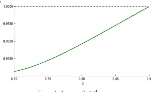
period (T = 0) about β, the average level of effort the regulator implements in period (T = 1), ¯e1, is depicted in Figure 1. The average level of effort is increasing in β and, as
discussed before, if the firm’s type is ¯β = 1, the regulator implements the first-best effort in (T = 1), regardless of the firm’s ex post typeθ.
Figure 1: Average effort ¯e1.
4.1.2 Investment
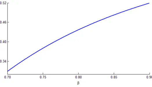
As shown in Figure 2, the first-best level of investmentI∗
is increasing and concave inβ. In Case (θ,β,IRep), the optimal level of investment I1 is increasing in β and there
is underinvestment except forβ = 1. To evaluate how serious is the underinvestment, we define the ratio
RI1(β) = I1(β)
I∗(β). (16)
Figure 3 depicts the proportion of investment in Case (θ,β,IRep) relative to the
that that the firm’s expected utility in period (T = 1), Eθ[U(θ, β)], is increasing, thus, by
Lemma 3 in the Appendix, we know that the solution in Case (θ,β,IRep) is implementable.
Figure 2: First-best level of investment.
Figure 3: Investment relative to the first-best.
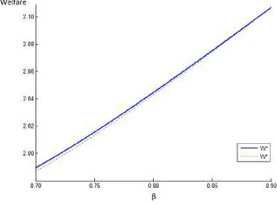
4.1.3 Welfare
The expected social welfare in period (T = 0) is increasing in β. In Case (θ,β,IRep)
the welfare W1 is always below the first-best level of social welfare W∗
, shown in Figure 4. As parameterβ increases, the effort implemented in Case (θ,β,IRep) gets closer to the
first-best e∗
and the investment I1 approaches I∗
. Thus, W1 gets closer to the first-best W∗
since the regulator must leave rent to the firm, the level of welfareW1 does not reach the
first-bestW∗
.
Figure 4: Welfare.
4.2
Violating the Spence-Mirrlees condition
According toAraujo and Moreira(2010), the single-crossing or Spence-Mirrlees con-dition (SMC) has been the the main assumption that allows us to fully characterize the solution of one-dimensional adverse selection or hidden information models.4 We say that
the SMC holds if the the preferences of the privately informed part are such that the marginal rates of substitution between a decision variable and money are increasing with respect to a one-dimensional parameter or type. Under the SMC, the implementable de-cisions are non-decreasing in type. In this subsection, we provide an example in which the SMC condition is violated, but we do not solve the regulator’s problem.
Suppose thatβis private information to the firm andθis observable for the regulator, and that there is an ex post IR constraint. Let ¯u > 0 be the firm’s reservation utility in both periods. We solved the regulator’s welfare maximization problem for this case in Subsection 3.3. As discussed before, in period (T = 1) the regulator optimally sets
4
U(θ, β) = ¯u for every β ∈B. Thus, we define
V(I, β, t0)≡Q(I, β)¯u+t0 (17)
as the firm’s utility in period (T = 0). In this case the SMC condition is
VβI =QβIu >¯ 0 (18)
which holds if QβI >0. Thus, Assumption 1 is the SMC in our model.
As noted before, the cross-derivative in our example isQβI(I, β) = [exp(−Iβ)/2][1− Iβ], which can be non-positive. In fact, the SMC condition in this case is violated in a natural way in our model. Since Q represents the probability of discovery, it is a limited variable. Thus, when Q is close enough to 1, the marginal effect of an increase in investment, QI, is decreasing in β. Hence, when the probability is close to 1, I and β become substitute inputs to Q.5 The solution when the SMC does not hold can be
characterized by using techniques developed inAraujo and Moreira(2010). However, the analysis when the SMC is violated is beyond the scope of this work.
5
5
Conclusions
In this work we characterized the optimal regulation of oil exploration and pro-duction under asymmetric information. We developed a simple two-period model that considers some important uncertainties in petroleum contracts, focusing on the issues re-lated to asymmetric information. In Section 3, we proved that the existence of asymmetric information only in the production period is irrelevant, since the regulator can implement the first-best outcome.
However, when the firm cannot commit to produce for bad realizations of θ, the expected level of social welfare decreases in the existence of asymmetric information in the exploration period. In this case, the regulator can no longer use the second period to extract the rent left to the firm when investment was made. Since the firm must be given a minimum level of utility in the production period, the regulator cannot share risks with the firm in an efficient way. furthermore, if there is asymmetric information in both periods, there is an interaction between incentive provision in each period. The effort contracted to the production period is a function of the investment realized in the exploration stage and its effectiveness parameter.
We also provided an example with numerical results. In that example, we pointed out that the Spence-Mirrlees (SMC) condition can be violated in our model. Moreover, it turns out that the violation of the SMC is the result of particular characteristics of petroleum contracts rather than an artificial construction.
References
Aghion, P. and L. Quesada(2010): Petroleum Contracts: What Does Contract
The-ory Tell Us?, MIT Press.
Araujo, A. and H. Moreira(2010): “Adverse selection problems without the
Spence-Mirrlees condition,”Journal of Economic Theory, 145, 1113–1141.
Laffont, J.-J. and J. Tirole (1993): A theory of incentives in procurement and
regulation, MIT Press.
Mirrlees, J.(1971): “An exploration in the theory of optimal income taxation,”Review
of Economic Studies, 38, 175–208.
Schotmuller, C.(2012): “Essays in Microeconomic Theory,”PhD Thesis, Tilburg
6
Appendix
Proof (optimal regulation under complete information): Since rents are costly, the regulator optimally sets U(β) = 0, for all β ∈ B. Thus, the welfare maximization problem is
max
I(·),e(·)Q(I(β), β)Eθ[p−(1 +λ)(θ−e(θ, β) +ψ(e(θ, β)))]−(1 +λ)I(β)
which is equivalent to
max
I(·) {maxe(·) Q(I(β), β)Eθ[p−(1 +λ)(θ−e(θ, β) +ψ(e(θ, β)))]−(1 +λ)I(β)}
The first-order condition (F OC) of the maximization problem inside the braces is
ψ′
(e(θ, β)) = 1
or
e(θ, β) =e∗
≡ψ′−1(1)
and the second-order conditons (SOC) are satisfied, since
−Q(I(β), β)(1 +λ)Eθ[ψ ′′
(e(θ, β))]<0
and the problem is concave in e. Hence, the constant level of effort e∗
is the solution to the problem. Thus, the regulator’s solves
max
I(·) Q(I(β), β)[p−(1 +λ)(Eθ[θ]−e ∗
+ψ(e∗
))]−(1 +λ)I(β)
The F OC to this problem is
QI(I(β), β)(p−(1 +λ)(Eθ[θ]−e ∗
+ψ(e∗
))) = 1 +λ (19)
and the SOC are satisfied, since
and the problem is concave inI. The inequality in (20) is a result of the assumption that
pis large enough so that is always worth producing oil.
Proof of Lemma 2: (N ecessity) Since there is no asymmetric information in the production period and rents are costly, the regulator can optimally setEθ[U(β, θ)] = ¯u >
0, for every β. Thus, the first-order condition of incentive compatibility (IC) in period (T = 0) implies
˙
U(β) = Qβ(I(β), β)¯u (IC0.a)
which is equivalent to
QI(I(β), β) ˙I(β)¯u+ ˙t0(β) = 0. (21)
The IC constraint also implies that, for everyβ,βˆ∈B, it must be true that
Q(I(β), β)¯u+t0(β)≥Q(I( ˆβ), β)¯u+t0( ˆβ)
Q(I( ˆβ),βˆ)¯u+t0( ˆβ)≥Q(I(β),βˆ)¯u+t0(β)
which implies
¯
u
Z βˆ
β
[QI(I( ˆβ), x)−QI(I(β), x)]dx≥0.
which can be written as
¯
u
Z βˆ
β
Z I( ˆβ)
I(β)
QβI(y, x)dydx ≥0 (22)
SinceQβI >0 by Assumption 1, the level of investment must be increasing inβ to satisfy
equation (22) and therefore (IC0.b) must hold.
(Suf f iciency) Suppose that (IC0.a) and (IC0.b) hold. Suppose by way of
contradic-tion that there is a type β that strictly preffers to announce type β′
6
= β. It must hold that
Q(I(β′
), β)¯u+t0(β′
and therefore
Z β′
β
[QI(I(x), β) ˙I(x)¯u+ ˙t0(x)]dx >0
By using equation (24), we have
Z β′
β
[QI(I(x), β) ˙I(x)¯u+ ˙t0(x)−(QI(I(x), x) ˙I(x)¯u+ ˙t0(x))]dx >0
which implies
¯
u
Z β′
β Z β
x
QβI(I(x), y) ˙I(x)dydx >0. (23)
However, this inequality cannot hold, and we obtain the contradiction. To see that, take
β′
≥ β. Then x ≥β and the inequality in (25) does not hold, since QβI >0 and ˙I ≥0.
The proof is analogous for β′ < β.6
Lemma 3 (Sufficient conditions for IC in the exploration period). If the firm’s expected utility in the production period is non-negative, the following conditions are sufficient to satisfy the (IC0)
˙
U(β) =Qβ(I(β), β) ¯U(β) (IC0.a)
˙
I(β)≥0 (IC0.b)
˙¯
U(β)≥0 (IC0.c)
where ¯U(β) =Eθ[U(θ, β)].
Proof: Suppose that the first-order condition (IC0.a) and the monotonicity conditions
(IC0.b) and (IC0.c) hold. The first-order condition (IC0.a) is equivalent to
QI(I(β), β) ˙I(β) ¯U(β) +Q(I(β), β) ˙¯U(β) + ˙t0(β) = 0 (24)
Suppose by way of contradiction that there is a type β that strictly preffers to
6
announce typeβ′
6
=β. It must hold that
Q(I(β′
), β) ¯U(β′
) +t0(β′
)> Q(I(β), β) ¯U(β) +t0(β)
and therefore
Z β′
β
[QI(I(x), β) ˙I(x) ¯U(x) +Q(I(x), β) ˙¯U(x) + ˙t0(x)]dx >0
By using equation (24), we have
Z β′
β
[QI(I(x), β) ˙I(x) ¯U(x) +Q(I(x), β) ˙¯U(x) + ˙t0(x)
−(QI(I(x), x) ˙I(x) ¯U(x) +Q(I(x), x) ˙¯U(x) + ˙t0(x))]dx > 0
which implies
Z β′
β Z β
x
[QβI(I(x), y) ˙I(x) ¯U(x) +Qβ(I(x), y) ˙¯U(x)]dydx >0 (25)
Hower, this inequality cannot hold, and we obtain the contradiction. To see that, take
β′
≥β. Then x≥β and the inequality in (25) does not hold, sinceQβI, Qβ >0, ˙I,U˙¯ ≥0
and ¯U is non-negative. The proof is analogous for β′ < β.
Proof of Proposition 6:
• Private information about β
Since ˙U ≥0, the ex ante IR constraint must be satisfied at the least efficient type
U(β)≥0. (IRex ante)
problem is
max
I(·),e(·),U(·)
Z β¯
β (
Q(I(β), β)Eθ[p−(1 +λ) [θ−e(θ, β) +ψ(e(θ, β))]]
−(1 +λ)I(β)−λU(β)
)
g(β)dβ
subject to (IC0.a), (IC0.b) and (IRex ante).
The regulator can implement e∗
, sinceθ is common knowledge. If the regulator sets
Eθ[U(θ, β)] = 0, then the IC constraint (IC0.a) is satisfied if ˙U(β) = 0. Hence, the
regulator optimally sets t0(β) = 0, then U(β) = 0 and, therefore, (IC0
.a) is satisfied
for every level of investment, with no rent left to the firm. Thus, the regulator can implement the first-best investment I∗
(β), which is increasing in β an satisfies (IC0.b), achieving the the first-best regulatory outcome.
There are many ways to implement Eθ[U(θ, β)] = 0. In particular, the regulator can
set t1(θ, β) =ψ(e∗
).
• Private information about θ
In this case, the regulator’s objective is to maximize the expected social welfare in (T = 0), subject to the ex ante individual rationality and the incentive compatibility constraints. The optimization problem is
max
I(·),e(·),U(·),t0(·)Q(I(β), β)Eθ[p−(1 +λ) (θ−e(θ, β) +ψ(e(θ, β)))]−λU(θ, β)] −(1 +λ)I(β)−λt0(β)
subject to
˙
U(θ, β) = −ψ′
(e(θ, β)) (IC1.a)
˙
e(θ, β)≤1 (IC1.b′)
It is straightforward to see that the first-best regulatory outcome can be achieved and therefore it is the solution to this welfare maximization problem. If the regulator sets and I(β) =I∗
(β) and e(θ, β) =e∗
, condition (IC1.b′) is satisfied. The regulator
can set t1(θ, β), such that (IC1
.a) is also satisfied and that Eθ[U(θ, β)] = 0, and t0(β) = 0. Thus, the firm’s expected utility is always 0, and the regulator leaves no
rent to the firm. Condition (IC1.a) determines that the firm’s utility in (T = 1) is
strictly decreasing inθ, therefore the firm gets negative utility if its type is inefficient in cost reduction (high θ).
• Private information about β and θ
If we assume that there is just an ex ante IR constraint, the regulator solves
max
I(·),e(·),U(·)
Z β¯
β (
Q(I(β), β)Eθ[p−(1 +λ) (θ−e(θ, β) +ψ(e(θ, β)))]
−(1 +λ)I(β)−λU(β)
)
g(β)dβ
subject to (IC0), (IC1.a),(IC1.b′) and
U(β)≥0. (IRex ante)
It is straightforward to see that the first-best regulatory outcome can be achieved and it is the solution to this program. If the regulator sets I(β) =I∗
(β), which is increasing inβ, and e(θ, β) =e∗
, conditions (IC0.b) and (IC1.b′) are satisfied. The regulator can set t1(θ, β) such that (IC1
.a) is also satisfied and that Eθ[U(θ, β)] = 0, which ensures that
condition (IC0.a) is satisfied. If the regulator also setst0(β) = 0, the ex ante IR is always
binding and no rent is left to the firm. Note that, if (IC0.a) and (IC0.b) are sufficient
conditions for incentive compatibility in period (T = 0) when Eθ[U(θ, β)] = 0.
As in the setting where just θ is private information to the firm, the negative utility the firm expects to get if it turns out to be a high θ type in (T = 1) compensates the positive utility of the lowθ types. For every announcement ˆβ of its parameter in (T = 0), the firm has the same expected utility (Eθ[U(θ,βˆ)] = 0) and therefore it is indifferent