Heat and mass transfer effect s on unsteady MHD flow of a chemically reacting fluid past an impulsively started vertical plate with radiation

International Journal of Advances in Applied Mathematics and Mechanics

Volume , )ssue : pp. - 5 Available online at www.ijaamm.com

IJAAMM

ISSN: 2347-2529

Heat and mass transfer effects on unsteady MHD flow of a

chemically reacting fluid past an impulsively started

vertical plate with radiation

M. Gnaneswara Reddy a, *

a

Department of Mathematics, Acharya Nagarjuna University Ongole Campus- - 523 001, A. P., India

Received 17 September 2013; Accepted (in revised version) 17 October 2013

A B S T R A C T

The objectives of the present study are to investigate thermal radiation of a viscous incompressible unsteady chemically reacting and hydromagnetic fluid flow past an impulsively started vertical plate with heat and mass transfer is analyzed. The fluid is a gray, absorbing-emitting but non-scattering medium and the Rosseland approximation is used to describe the radiative heat flux in the energy equation. The governing equations are solved using an implicit finite-difference scheme of Crank-Nicolson type. Numerical results for the transient velocity, the temperature, the concentration, the local as well as average skin-friction, the rate of heat and mass transfer are shown graphically. It is found that as small values of the Prandtl number and radiation parameter N, the velocity and temperature of the fluid increase sharply neat the cylinder as the time t increase, which is totally absent in the absence of radiation effects. It is observed that the presence of chemical reaction parameter K(>0) leads to decrease in the velocity field and concentration and rise in the thermal boundary thickness.

Keywords: MHD; Heat transfer; Radiation; Finite-difference Scheme; vertical plate.

MSC 2010 codes:80A20, 65L12.

© 2013 IJAAMM

Nomenclature

0

B The magnetic induction

C′ Species concentration

C Dimensionless species concentration

Gr Thermal Grashof number

Gc Modified Grashof number

g Acceleration due to gravity

K Chemical reaction parameter

M Magnetic parameter

N Radiation parameter

Nu Average Nusselt number

*

x

Nu Local Nusselt number

Pr Prandtl number

r

q Radiative heat flux

Sc Schmidt number

Sh Average Sherwood number

X

Sh Local Sherwood number

T

t Time

0

u Velocity of the plate

V

U, Dimensionless velocity components in X,R directions respectively

X Dimensionless axial co-ordinate

Greek symbols

α

β Volumetric coefficient of thermal expansion

*

β Volumetric coefficient of expansion with concentration

e

k Mean absorption coefficient

ν Kinematic viscosity ρ Density

σ Electrical conductivity

s

σ Stefan-Boltzmann constant

x

τ Local skin-friction τ Average skin-friction

Subscripts

w

∞ Free-stream condition

1 Introduction

The study of magnetohydrodynamics (MHD) plays an important role in agriculture, engineering and petroleum industries. The problem of free convection under the influence of a magnetic field has attracted the interest of many researchers in view of its applications in geophysics and astrophysics. Soundalgekar et al. (1979) analyzed the problem of free convection effects on Stokes problem for a vertical plate under the action of transversely applied magnetic field. Elbashbeshy (1997) studied the heat and mass transfer along a vertical plate under the combined buoyancy effects of thermal and species diffusion, in the presence of magnetic field. Helmy (1998) presented an unsteady two-dimensional laminar free convection flow of an incompressible, electrically conducting (Newtonian or polar) fluid through a porous medium bounded by an infinite vertical plane surface of constant temperature.

and mass transfer plays an important role are designing of chemical processing equipment, formation and dispersion of fog, distribution of temperature and moisture over agricultural fields and groves of fruit trees, crop damage due to freezing, and environmental pollution. In this context the first systematic study of mass transfer effects on free convection flow past a semi-infinite vertical plate was presented by Gebhart and Pera (1971), who presented a

similarity solution to this problem and introduced a parameter N which is a measure of

relative importance of chemical and thermal diffusion in causing the density difference that

drives the flow. The parameter N is positive when both effects combined to drive the flow and

it is negative when these effects are opposed. Callahan and Marner (1976) first studied the transient free convection flow past a semi-infinite plate by explicit finite difference method. They also considered the presence of species concentration. However this analysis is not applicable for fluids whose Prandtl numbers are different from unity. Soundalgekar and Ganesan [6] solved the problem of transient free convective flow past a semi-infinite vertical flat plate, taking into account mass transfer by an implicit finite difference method of

Crank-Nicolson type. In their analysis they observed that an increase in N leads to an increase in the

velocity but a decrease in the temperature and concentration. Muthucumarswamy and Ganesan (1998) solved the problem of unsteady flow past an impulsively started semi-infinite vertical plate with heat and mass transfer.

The role of thermal radiation is of major importance in some industrial applications such as glass production and furnace design and in space technology applications, such as cosmical flight aerodynamics rocket, propulsion systems, plasma physics and space craft reentry aerothermodynamics which operate at high temperatures. When radiation is taken into account, the governing equations become quite complicated and hence many difficulties arise while solving such equations. Greif et al. (1971) shown that in the optically thin limit the physical situation can be simplified, and then they derived exact solution to fully developed vertical channel for a radiative fluid. Hossain and Takhar (1996) studied the radiation effects on mixed convection along a vertical plate with uniform surface temperature using Keller Box finite difference method. Abd El-Naby et al. (2003) studied the effects of radiation on unsteady free convective flow past a semi-infinite vertical plate with variable surface temperature using Crank-Nicolson finite difference method. They observed that, both the velocity and temperature are found to decrease with an increase in the temperature exponent. Chamkha et al. (2001) analyzed the effects of radiation on free convection flow past a semi-infinite vertical plate with mass transfer, by taking into account the buoyancy ratio parameter

N. In their analysis they found that, as the distance from the leading edge increases, both the

velocity and temperature decrease, whereas the concentration increases.

The aim of the present paper is to study the unsteady heat and mass transfer MHD flow of a chemically reacting fluid past an impulsively started vertical plate with radiation. The equations of continuity, linear momentum, energy and species concentration, which govern the flow field are solved by using an implicit finite difference scheme of Crank-Nicolson type. The behaviour of the velocity, temperature, concentration, skin-friction, Nusselt number and Sherwood number has been discussed for variations in the governing parameters.

2 Mathematical

analysis

impulsively started vertical plate is considered. The x-axis is taken along the plate in the upward direction and the y-axis is taken normal to it. Initially, it is assumed that the plate and the fluid are at the same temperature T_∞′ and concentration level C_∞′ everywhere in the fluid.

At time t′ >0, the plate starts moving impulsively in the vertical direction with constant

velocity u0 against the gravitational field. Also, the temperature of the plate and the

concentration level near the plate are raised to T_w′ and C_w′ respectively and are maintained

constantly thereafter. It is assumed that the concentration C′ of the diffusing species in the

binary mixture is very less in comparison to the other chemical species, which are present, and hence the Soret and Dufour effects are negligible. Then, under the above assumptions, the governing boundary layer equations with Boussinesq’s approximation are

0

u v

x y

∂ ∂

+ =

∂ ∂ (1)

2 2

* 0

2

( ) ( )

u u u u B

u v g T T g C C u

t x y y

σ

β β ν

ρ

∞ ∞

∂ ∂ ∂ ∂

′ ′ ′ ′

+ + = − + − + −

′

∂ ∂ ∂ ∂ (2)

2 2

1 _r

p

T T T T q

u v

t x y α y ρc y

′ ′ ′ ′

∂ ∂ ∂ ∂ ∂

+ + = −

′

∂ ∂ ∂ ∂ ∂ (3)

2 2 l

C C C C

u v D k C

t x y y

′ ′ ′ ′

∂ ∂ ∂ ∂

′

+ + = −

′

∂ ∂ ∂ ∂ (4)

The initial and boundary conditions are

0

0: 0, 0, ,

0 : , 0, , 0

0, , 0

0, ,

w w

t u v T T C C

t u u v T T C C at y

u T T C C at x

u T T C C as y

∞ ∞

∞ ∞

∞ ∞

′≤ = = ′= ′ ′= ′ ⎫

⎪

′> = = ′= ′ ′= ′ = _⎪

⎬

′ ′ ′ ′

= = = = _⎪

⎪

′ ′ ′ ′

→ → → → ∞ _⎭

(5)

By using the Rosseland approximation (Brewster 1992), the radiative heat flux q_r is given by

4

4 3

s r

e

T q

k y

σ ∂ ′

= −

∂ (6)

where σ_s is the Stefan-Boltzmann constant and k_e - the mean absorption coefficient. It

should be noted that by using the Rosseland approximation the present analysis is limited to optically thick fluids. If temperature differences within the flow are sufficiently small, then

Equation (6) can be linearized by expanding _T′4 _{into the Taylor series about}

∞′

T , which after

4 3 4

4 3

T′ ≅ T T_∞′ ′− T_∞′ (7)

In view of Equations (6) and (7), Equation (3) reduces to

2 3 2

2 2

16 3

s

e p

T T T T T T

u v

t x y y k c y

σ α ρ ∞ ′ ′ ′ ′ ′ ′ ∂ ∂ ∂ ∂ ∂ + + = + ′

∂ ∂ ∂ ∂ ∂ (8)

Local and average skin-friction are given respectively by

0 x y u y τ µ = ⎛∂ ⎞ ′ = − _{⎜ ⎟} ∂

⎝ ⎠ (9)

0 0 1 L L y u dx L y τ µ = ⎛ ⎞ − ∂ = _{⎜ ⎟} ∂ ⎝ ⎠

∫

Local and average Nusselt number are given respectively by

0 y x w T x y Nu T T = ∞ ′ ⎛∂ ⎞ − _{⎜ ⎟} ∂ ⎝ ⎠ =

′− ′ (11)

0 0 ( ) L L _w y T

Nu T T dx

y ₌ ∞

⎡_{⎛∂ ′⎞} ⎤ ′ ′ = − ⎢_{⎜ ⎟} − ⎥ ∂ ⎝ ⎠ ⎢ ⎥ ⎣ ⎦

∫

Local and average Sherwood number are given respectively by

0 y x w C x y Sh C C = ∞ ′ ⎛∂ ⎞ − _{⎜ ⎟} ∂ ⎝ ⎠ =

′ − ′ (13)

0 0 ( ) L L _w y C

Sh C C dx

y ∞ = ⎡_{⎛∂ ′⎞} ⎤ ′ ′ = − ⎢_{⎜ ⎟} − ⎥ ∂ ⎝ ⎠ ⎢ ⎥ ⎣ ⎦

∫

On introducing the following non-dimensional quantities

2 2

0 0 0 0

2

0 0 0

*

3 3 3

0 0 2 0 , , , , , ( ) ( ) , , , 4

, , Pr , ,

w w e

s

l

w w

x u y u t u u v B

X Y t U V M

u u u

g T T g C C k k

Gr Gc N

u u T

T T C C K

T C Sc K

T T C C D u

σ ν

ν ν ν

ν β ν β

σ

ν ν ν

Equations (1), (2), (8) and (4) are reduced to the following non-dimensional form 0 U V X Y ∂ ∂ + =

∂ ∂ (16)

2 2

U U U U

U V Gr T Gc C MU

t X Y Y

∂ ∂ ∂ ∂

+ + = + + −

∂ ∂ ∂ ∂ (17)

(17) 2 2 1 4 1 Pr 3

T T T T

U V

t X Y N Y

∂ ∂ ∂ ⎛ ⎞∂

+ + = _⎜ + _⎟

∂ ∂ ∂ ⎝ ⎠∂ (18)

(18)

2 2

1

C C C C

U V KC

t X Y Sc Y

∂ ∂ ∂ ∂

+ + = −

∂ ∂ ∂ ∂ (19)

The corresponding initial and boundary conditions are

0: 0, 0, 0, 0

0 : 1, 0, 1, 1 0

0, 0, 0 0

0, 0, 0

t U V T C

t U V T C at Y

U T C at X

U T C as Y

≤ = = = = ⎫

⎪

> = = = = = ⎪

⎬

= = = = _⎪

⎪

→ → → → ∞ _⎭

(20)

where Gr is the thermal Grashof number, Gc - the solutal Grashof number, M - the magnetic

field parameter, Pr - the fluid Prandtl number, Sc - the Schmidt number and N - the

radiation parameter, K - the chemical reaction parameter.

Local and average skin-friction in non-dimensional form are

2 0 0 X Y U u Y τ τ ρ ₌ ′ ⎛∂ ⎞ = = −_{⎜ ⎟} ∂

⎝ ⎠ (21)

1

0 Y 0 U dX Y τ = ⎛∂ ⎞ = − _{⎜ ⎟} ∂ ⎝ ⎠

∫

Local and average Nusselt number in non-dimensional form are

0 X Y T Nu X Y ₌ ⎛∂ ⎞ = − _{⎜ ⎟} ∂

⎝ ⎠ (23)

1

0 Y 0 T Nu dX Y ₌ ⎛∂ ⎞ = − _{⎜ ⎟} ∂ ⎝ ⎠

∫

0 X Y C Sh X Y ₌ ⎛∂ ⎞ = − _{⎜ ⎟} ∂

⎝ ⎠ (25)

1

0 Y 0 C Sh dX Y ₌ ⎛∂ ⎞ = − _{⎜ ⎟} ∂ ⎝ ⎠

∫

3 Numerical

technique

In order to solve the unsteady, non-linear coupled Equations (16) - (19) under the conditions (20), an implicit finite difference scheme of Crank-Nicolson type has been

employed. The region of integration is considered as a rectangle with sides X_max(=1) and

max

Y (=14), where Y_maxcorresponds toY = ∞, which lies very well outside the momentum,

energy and concentration boundary layers. The maximum of Y was chosen as 14 after some preliminary investigations, so that the last two of the boundary conditions (20) are satisfied within the tolerance limit 10-5.

The finite difference equations corresponding to Equations (16) - (19) are as follows

1 1 1 1 1 1

, 1, , 1, , 1 1, 1 , 1 1, 1 , , 1 , , 1

0

4 2

n n n n n n n n n n n n

i j i j i j i j i j i j i j i j i j i j i j i j

U U U U U U U U V V V V

X Y

+ + + + + +

− − − − − − − − − −

⎡ − + − + − + − ⎤ ⎡ − + − ⎤

⎣ ⎦ ⎣₊ ⎦₌

Δ Δ (27)

1 1 1 1 1

, , , 1, , 1, , 1 , 1 , 1 , 1

, ,

1 1 1 1 1 1

, , , , , 1 , , 1 , 1 ,

2 4

2 2

2 2

n n n n n n n n n n

i j i j n i j i j i j i j n i j i j i j i j

i j i j

n n n n n n n n n

i j i j i j i j i j i j i j i j i j

U U U U U U U U U U

U V

t X Y

T T C C U U U U U

Gr Gc + + + + + − − + − + − + + + + + + − + + ⎡ − ⎤ ⎡ − + − ⎤ ⎡ − + − ⎤ ⎣ ⎦₊ ⎣ ⎦₊ ⎣ ⎦

Δ Δ Δ

⎡ + ⎤ ⎡ + ⎤ − + + − +

⎣ ⎦ ⎣ ⎦

= + + ₂ , 1

1 , , 2( ) 2 n i j n n

i j i j

U Y M U U + + ⎡ ⎤ ⎣ ⎦ Δ ⎡ ⎤ − _⎣ + _⎦ (28)

1 1 1

1

, 1, , 1, , , 1 , 1 , 1

, ,

, ,

1 1 1

, 1 , , 1 , 1 , , 1 2 [ ] 2 4 2 2 1 4 1

Pr 3 2( )

n n n n n n n

n n

i j i j i j i j i j i j i j i j

i j i j n n

i j i j

n n n n n n

i j i j i j i j i j i j

T T T T T T T T

T T

U V

t X Y

T T T T T T

N Y + + + + − − − + − + + + − + − + ⎡ − + − ⎤ ⎡ − + − ⎤ − _{⎣ ⎦ ⎣ ⎦} + +

Δ Δ Δ

⎡ − + + − + ⎤ ⎛ ⎞ ⎣ ⎦ = _⎜ + _⎟ Δ ⎝ ⎠ (29)

1 1 1 1

1

, 1, , 1, , 1 , 1 , 1 , 1

, ,

, ,

1 1 1

, 1 , , 1 , 1 , , 1 1

, , 2 [ ] 2 4 2 2 1

2( ) 2

n n n n n n n n

n n

i j i j i j i j i j i j i j i j

i j i j n n

i j i j

n n n n n n

i j i j i j i j i j i j n n

i j i j

C C C C C C C C

C C

U V

t X Y

C C C C C C _K

C C Sc Y + + + + + − − + − + − + + + − + − + + ⎡ − + − ⎤ ⎡ − + − ⎤ − _{⎣ ⎦ ⎣ ⎦} + +

Δ Δ Δ

⎡ − + + − + ⎤

⎣ ⎦ _{⎡ ⎤}

= − _⎣ + _⎦

Δ

Here, the subscript i - designates the grid point along the X - direction, j - along the Y-

direction and the superscript n along the t - direction. An appropriate mesh size considered for

the calculation is ΔX = 0.05, ΔY = 0.25, and time step Δt = 0.01. During any one-time step,

the coefficients U_in_,j and V_i,n_j appearing in the difference equations are treated as constants.

The values of U, V, TandC are known at all grid points at t = 0 from the initial conditions.

The computations of U, V, T andC at time level (n+1) using the known values at previous

time level (n) are calculated as follows.

The finite difference Equation (30) at every internal nodal point on a particular i -

level constitute a tri-diagonal system of equations. Such a system of equations is solved by

Thomas algorithm as described in Carnahan et al. (1996). Thus, the values of C are found at

every nodal point on a particular i at (n+1)th time level . Similarly, the values of T are

calculated from the Equation (29). Using the values of C and T at (n+1)th time level in the

Equation (28), the values of U at (n+1)th time level are found in a similar manner. Thus the

values of C, T andU are known on a particular i - level. The values of V are calculated

explicitly using the Equation (27) at every nodal point on a particular i - level at (n+1)th time level. This process is repeated for various i - levels. Thus, the values of C,T,U and V are known at all grid points in the rectangular region at (n+1)th time level.

Computations are carried out till the steady state is reached. The steady state solution

is assumed to have been reached, when the absolute difference between the values of U as

well as temperature T and concentration C at two consecutive time steps are less than 10-5 at

all grid points. The derivatives involved in the Equations (21) - (26) are evaluated using five-point approximation formula and the integrals are evaluated using Newton-Cotes closed integration formula.

4 Results and discussions

A representative set of numerical results is shown graphically in Figs.1-10, to illustrate

the influence of physical parameters viz., radiation parameter N, Grashof number Gr, mass

Grashof number Gc, Magnetic field parameter M , Schmidt number Sc and chemical reaction

parameter K on the velocity, temperature and concentration, skin-friction, Nusselt number and

Sherwood number. The value of the Prandtl number Pr is chosen to be 0.71(i.e., for air) and

the other parameters are arbitrarily chosen.

The transient velocity profiles for different values of Gr, Gc,M ,N, Sc and K at a

particular time t = 1.0 has been shown in Fig.1. It is observed that the transient velocity

increases with the increase in Gr or Gc. There is a fall in transient velocity with the increase

inM , N, Sc or K. In Fig.2, the transient and steady state velocity profiles are presented for

different values M, N, Sc, K and the buoyancy force parameters Gr or Gc. The steady state

velocity increases with the increase in Gr or Gc. The time required to reach the steady state

and the velocity decreases with the increase in M, N, Sc and K.

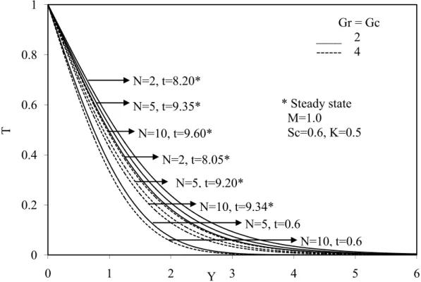
Fig .3 shows the temperature decreases with the increasing values of Gr or Gc. It can

also be seen that the time required to reach the steady state temperature is more at higher

From Figs.1 to 3, it is observed that, owing to an increase in the value of radiation

parameter N, the velocity and temperature decrease accompanied by simultaneous reductions

in both momentum and thermal boundary layers. However the time taken to reach the steady state increases as N increases.

The transient concentration profiles for Pr = 0.71, Gr = Gc(=2), N = 5,10 and Sc = 0.6 and 2.0 are shown in Fig. 4. It is observed that for small values of Sc = 0.6,K =0.5 and N =

5, the time required to reach the steady state is 8.10, where as when N = 10, under similar

conditions, the time required to reach the steady state is 8.31 from which it is concluded that

for higher values of N, the time taken to reach the steady state is more when Sc is small. It is

also observed that increasing values of N corresponds to a thicker concentration boundary

layer relative to the momentum boundary layer. Hence, it can be noted that at larger Sc, the

time required to reach the steady state is less as compared to that at low values of Sc. Also, an

increase in Sc or K leads to a fall in concentration.

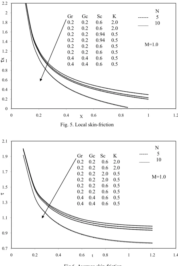
Steady state local skin-friction τ_X profiles are shown in Fig.5. The local shear stress

X

τ increases with the increase in Sc or K, where as it deceases with the increase in Gr or Gm.

It is also observed that the local skin-friction τ_X increases as the radiation parameter N

increases. The average values of skin-friction τ are plotted in Fig.6. It is observed that

decreases with the increase in Gr or Gm throughout the transient period and at the steady state

level. It is also observed that the average skin-friction τ increases as the radiation parameter N

increases. The average skin-friction increases with increasing Sc or K. The local Nusslet

number Nu_X for different Gr, Gm, N, Sc and K are shown in Fig.7. The local heat transfer

rate Nu_X decreases with the increase in Sc or K, whereas it increases with the increase in Gr

or Gm. Also it is found that as the radiation parameter N increases the local Nusselt number

X

Nu increases. The average values of Nusselt number Nu are shown in Fig.8. It is noticed

that the average Nusselt number Nu increases with the increase in Gr or Gm or N, whereas it

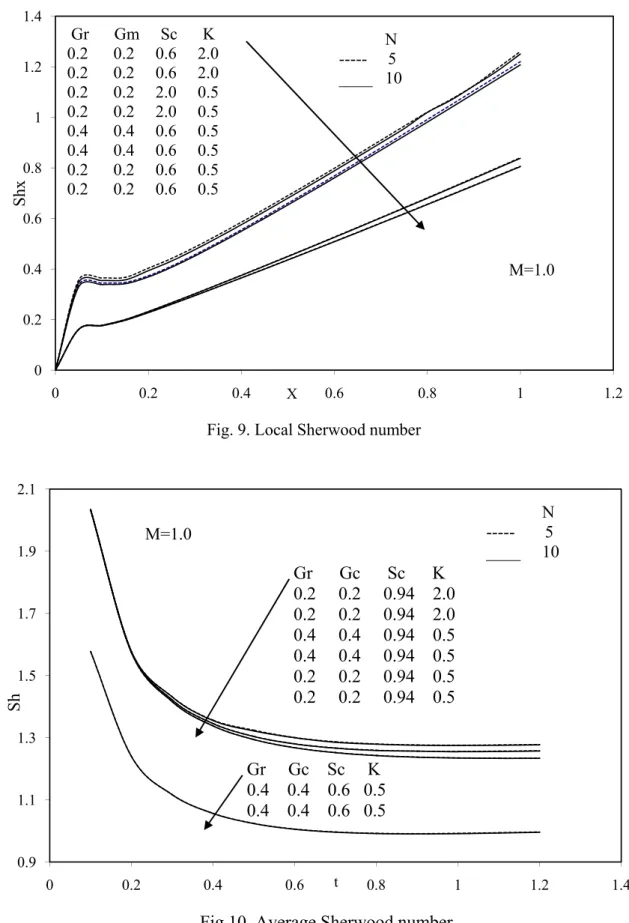
increases with the decrease in Sc or K. The local Sherwood number Sh_X is plotted in Fig.9. It

is observed that Sh_X increases with the increase in Sc or K, where as it decreases with the

increase in Gr, Gm or N. The average values of Sherwood number Sh are plotted in Fig.10. It

5 Figures

0 0.2 0.4 0.6 0.8 1 1.2 1.4 1.6

0 1 2 _Y 3 4 5

U

Gr Gc M N Sc K 2.0 2.0 1.0 2.0 0.6 0.5 -- I 4.0 2.0 1.0 2.0 0.6 0.5 -- II 2.0 4.0 1.0 2.0 0.6 0.5 -- III 2.0 2.0 2.0 5.0 0.6 0.5 -- IV 2.0 2.0 1.0 2.0 0.94 0.5 -- V 2.0 2.0 1.0 2.0 0.6 2.0 -- VI

t = 1.0 II

III

I

VI

IV

V

Fig. 1. Transient velocity profiles at X=1.0 for different Gr, Gc, M, N, Sc,

0 0.2 0.4 0.6 0.8 1 1.2 1.4 1.6 1.8

0 1 2 _Y 3 4 5 6

U

Gr Gc M N Sc K t

2.0 2.0 1.0 2.0 0.6 0.5 0.40 -- I 2.0 2.0 1.0 2.0 0.6 0.5 8.45* -- II 4.0 4.0 1.0 2.0 0.6 0.5 0.50 -- III 4.0 4.0 1.0 2.0 0.6 0.5 8.20* -- IV 2.0 2.0 2.0 5.0 0.6 0.5 0.45 -- V 2.0 2.0 1.0 5.0 0.6 0.5 8.10* -- VI 2.0 2.0 1.0 2.0 2.0 2.0 0.75 -- VII 2.0 2.0 1.0 2.0 2.0 2.0 8.90* --VIII IV

II VII

III

VI

VII I

V

0 0.2 0.4 0.6 0.8 1

0 1 2 3 4 5 6

T

Y

Fig.3. Temperature profiles at X=1.0 for different Gr, Gc, N N=2, t=8.20*

N=5, t=9.35*

N=10, t=9.60*

N=2, t=8.05*

N=5, t=9.20*

N=10, t=9.34* N=5, t=0.6

N=10, t=0.6 Gr = Gc ____ 2

--- 4

* Steady state M=1.0

Sc=0.6, K=0.5

0 0.2 0.4 0.6 0.8 1

0 1 2 3 4

C

Y

Sc K t 0.6 0.5 8.31*

0.6 0.5 8.10* 2.0 2.0 7.86* 2.0 2.0 7.90* 2.0 2.0 0.75 2.0 2.0 0.75

N --- 5 _____ 10

Gr=Gc=2.0 M=1.0

* Steady state

0 0.2 0.4 0.6 0.8 1 1.2 1.4 1.6 1.8 2 2.2

0 0.2 0.4 _X 0.6 0.8 1 1.2

Gr Gc Sc K 0.2 0.2 0.6 2.0 0.2 0.2 0.6 2.0 0.2 0.2 0.94 0.5 0.2 0.2 0.94 0.5 0.2 0.2 0.6 0.5 0.2 0.2 0.6 0.5 0.4 0.4 0.6 0.5 0.4 0.4 0.6 0.5

N

--- 5

____ 10

Fig. 5. Local skin-friction

τ

x

M=1.0

0.7 0.9 1.1 1.3 1.5 1.7 1.9 2.1

0 0.2 0.4 0.6 t 0.8 1 1.2 1.4

Fig.6. Average skin-friction

τ

Gr Gc Sc K 0.2 0.2 0.6 2.0 0.2 0.2 0.6 2.0 0.2 0.2 2.0 0.5 0.2 0.2 2.0 0.5 0.2 0.2 0.6 0.5 0.2 0.2 0.6 0.5 0.4 0.4 0.6 0.5 0.4 0.4 0.6 0.5

N

--- 5

____ 10

0 0.05 0.1 0.15 0.2 0.25 0.3 0.35 0.4 0.45

0 0.2 0.4 X 0.6 0.8 1 1.2

Gr Gc Sc K 0.4 0.4 0.6 0.5 0.2 0.2 0.6 0.5 0.2 0.2 0.94 0.5 0.2 0.2 0.6 2.0 0.4 0.4 0.6 0.5 0.2 0.2 0.6 0.5 0.2 0.2 0.94 0.5 0.2 0.2 0.6 2.0

N

--- 5

____ 10

Fig. 7. Local Nusselt number

Nu

x

M=1.0

0.7 0.8 0.9 1 1.1 1.2 1.3 1.4 1.5 1.6

0 0.2 0.4 0.6 _t 0.8 1 1.2 1.4

Fig. 8. Average Nusselt number Gr Gc Sc K 0.4 0.4 0.6 0.5 0.2 0.2 0.6 0.5 0.2 0.2 0.94 0.5 0.2 0.2 0.6 2.0

N --- 5 ____ 10

N

u

0 0.2 0.4 0.6 0.8 1 1.2 1.4

0 0.2 0.4 X 0.6 0.8 1 1.2

Gr Gm Sc K 0.2 0.2 0.6 2.0 0.2 0.2 0.6 2.0 0.2 0.2 2.0 0.5 0.2 0.2 2.0 0.5 0.4 0.4 0.6 0.5 0.4 0.4 0.6 0.5 0.2 0.2 0.6 0.5 0.2 0.2 0.6 0.5

N

--- 5

____ 10

Fig. 9. Local Sherwood number

Shx

M=1.0

0.9 1.1 1.3 1.5 1.7 1.9 2.1

0 0.2 0.4 0.6 t 0.8 1 1.2 1.4

Fig.10. Average Sherwood number Gr Gc Sc K 0.2 0.2 0.94 2.0 0.2 0.2 0.94 2.0 0.4 0.4 0.94 0.5 0.4 0.4 0.94 0.5 0.2 0.2 0.94 0.5 0.2 0.2 0.94 0.5

Gr Gc Sc K 0.4 0.4 0.6 0.5 0.4 0.4 0.6 0.5

N --- 5 ____ 10

S

h

References

Abd El-Naby, M. A., Elsayed M. E., Elbarbary and Nader, Y. A. (2003): Finite difference solution of radiation effects on MHD free convection flow over a vertical plate with variable surface temperature, J. Appl. Math. 2, pp. 65-86.

Brewster, M. Q. (1992): Thermal radiative transfer and properties, John Wiley & Sons. Inc., New York.

Callahan, G. D. and Marner, W. J. (1976): Transient free convection with mass transfer on an isothermal vertical flat plate, Int. J. Heat Mass Transfer 19, pp. 165-174.

Carnahan, B., Luther, H.A. and Willkes, J. O. (1969): Applied numerical methods, John Wiley and sons, New York.

Chamkha, A. J., Takhar, H. S. and Soundalgekar, V. M. (2001): Radiation effects on free convection flow past a semi-infinite vertical plate with mass transfer, Chem. Engg. J. 84, pp. 335-342.

Elbashbeshy, M. A. (1997): Heat and mass transfer along a vertical plate surface tension and concentration in the presence of magnetic field, Int. J. Eng.Sci. 34(5), pp. 515-522.

Gebhart, B. and Pera, L. (1971): The nature of vertical natural convection flows resulting form the combined buoyancy effects of thermal and mass diffusion, Int. J. Heat Mass Transfer 14, pp. 2025-2050.

Grief, R., Habib, I. S. and Lin, L. C. (1971): Laminar convection of radiating gas in a vertical channel, J. Fluid. Mech. 45, pp. 513-520.

Helmy, K. A. (1998): MHD unsteady free convection flow past a vertical porous plate, ZAMM 78, pp. 255-270.

Hossain, M. A., and Takhar,.H. S. (1996): Radiation effects on mixed convection along a vertical plate with uniform surface temperature, Heat Mass Transfer 31, pp. 243-248.

Muthucumarswamy, R. and Ganesan, P. (1998): Unsteady flow past an impulsively started vertical plate with heat and mass transfer, Heat and Mass transfer 14, pp. 187-193.

Soundalgekar, V. M., Gupta, S. K. and Birajdar, N. S. (1979): Effects of mass transfer and free effects on MHD Stokes problem for a vertical plate, Nucl.Eng.Des. 53, pp. 309-346.