AN EFFICIENT INITIALIZATION METHOD FOR K-MEANS CLUSTERING OF
HYPERSPECTRAL DATA
A. Alizade Naeini a , A. Jamshidzadeh b, *, M. Saadatseresht a, S. Homayouni c
a Department of Geomatic Engineering, Faculty of Engineering, University of Tehran, Tehran, Iran - (a.alizadeh, msaadat)@ut.ac.ir b Department of Geomatic Engineering, Faculty of Engineering, University of Bojnord, Bojnord, Iran - [email protected]
c Department of Geography, University of Ottawa, Ottawa, Canada - [email protected]
KEY WORDS: K-means, Clustering Initialization methods, Unmixing, MVES, Hyperspectral data
ABSTRACT:
K-means is definitely the most frequently used partitional clustering algorithm in the remote sensing community. Unfortunately due to its gradient decent nature, this algorithm is highly sensitive to the initial placement of cluster centers. This problem deteriorates for the high-dimensional data such as hyperspectral remotely sensed imagery. To tackle this problem, in this paper, the spectral signatures of the endmembers in the image scene are extracted and used as the initial positions of the cluster centers. For this purpose, in the first step, A Neyman–Pearson detection theory based eigen-thresholding method (i.e., the HFC method) has been employed to estimate the number of endmembers in the image. Afterwards, the spectral signatures of the endmembers are obtained using the Minimum Volume Enclosing Simplex (MVES) algorithm. Eventually, these spectral signatures are used to initialize the k-means clustering algorithm. The proposed method is implemented on a hyperspectral dataset acquired by ROSIS sensor with 103 spectral bands over the Pavia University campus, Italy. For comparative evaluation, two other commonly used initialization methods (i.e., Bradley & Fayyad (BF) and Random methods) are implemented and compared. The confusion matrix, overall accuracy and Kappa coefficient are employed to assess the methods’ performance. The evaluations demonstrate that the proposed solution outperforms the other initialization methods and can be applied for unsupervised classification of hyperspectral imagery for landcover mapping.
1. INTRODUCTION
Classification can be categorized into two main groups of supervised and unsupervised classification methods. Although supervised methods lead to the better results, unsupervised or clustering techniques have been attracted a lot of attentions because they don’t need any training data and procedure (Melgani and Pasolli, 2013).
Among different clustering algorithms, partitional methods are one of the best techniques for high-dimensional data, e.g., hyperspectral data. This is mainly because they have lower complexity (Celebi et al., 2013). The k-means algorithm is undoubtedly the most widely used partitional clustering algorithm (Jain, 2010). However, k-means has two significant disadvantages. First, it is sensitive to the outlier and noise. Second, it is highly sensitive to the selection of the initial clusters. Adverse effects of improper initialization include empty clusters, slower convergence, and a higher chance of getting stuck in bad local minima. Fortunately, these two drawbacks can be alleviated using an appropriate initialization method (Celebi et al., 2013). The problem of the initialization can be addressed by either deterministic (Celebi et al., 2013) or heuristic methods (Abraham et al., 2008). Although heuristic methods like particle swarm optimization (PSO) may lead to the best results, they are time-consuming and may have less stability in high-dimensional data. Accordingly, deterministic methods have priority if they lead to an acceptable result.
To address the initialization problem, different methods have been proposed especially for hyperspectral imagery. In (Sun et al., 2013), an artificial bee colony algorithm is used to find the appropriate position of cluster centers in hyperspectral data. In another similar work, (Namin et al., 2013) used the PSO clustering algorithm in Minimum noise fraction space. The comparison of their results with the K-means clustering method
* Corresponding author.
showed better performance for the PSO clustering in minimum noise fraction feature space. In (Celebi et al., 2013), the authors compared different initialization methods for k-means. Although, they have shown Bradley and Fayyad’s method is one of the best initialization methods, it was also demonstrated that the popular initialization methods often perform poorly and that there are in fact strong alternatives to these methods.
In this paper, a new initialization method for hyperspectral data clustering using k-means has been proposed. In this method, first, the number of endmembers is estimated by using the HFC (Harsanyi et al., 1993) technique. Then the spectral signature of endmembers (i.e., initial position of cluster centers) is obtained based on the MVES method.
The rest of the paper is organized as follows. Section 2 presents a summary of k-means, HFC and MVES algorithms. Section 3 introduces our proposed method. Section 4 describes the experimental setup and results. Lastly, section 5 gives our conclusion.
2. THEORETICAL BACKGROUND
2.1 K-Means Clustering
K-means clustering (MacQueen, 1967) is a method commonly used to automatically partition a dataset into K groups. It proceeds by selecting K initial cluster centers and then iteratively refining them as follows. 1) First, each point is assigned to its closest cluster center, 2) Each cluster center Cj is updated to be the mean of its constituent points (Wagstaff et al., 2001). From the mathematical perspective, given a data set X =
� = �
�
= , � � = ∅ for 1 ≤ i ≠ j ≤ K. This algorithm generates clusters by optimizing a criterion function. The most intuitive and frequently used criterion function is the Sum of Squared Error (SSE) given by:
��E = ∑ ∑ ‖� − � ‖
� ∈� �
=
(1)
Where ‖. ‖ denotes the Euclidean (ℒ ) norm and � =
|� | ∑� ∈� � is the centroid of cluster � whose cardinality is |� |. The optimization of (1) is often referred to as the minimum SSE clustering (MSSC) problem (Celebi et al., 2013) . Based on application, different similarity measures can be used instead of Euclidean distance (ED). In this study, Spectral similarity value (SSV) (Farifteh et al., 2007), as one of the most successful similarity measures in hyperspectral data (Homayouni and Roux, 2004), is used. SSV combines brightness and shape similarity. It is a combined measure of Pearson correlation (PC) and ED measures.
2.2 HFC Method
A Neyman–Pearson detection theory-based eigen-thresholding method, referred to as the HFC method, was developed to determine the number of endmembers, which called Virtual Dimensionality (VD), in AVIRIS data (Harsanyi et al., 1993). It first calculated the sample correlation matrix RL×L and sample covariance matrix KL×L and then found the difference between their corresponding eigenvalues, where L is the number of spectral band in the image. Let {λ’1≥ λ’2≥ … ≥ λ’L} and {λ1≥ λ2≥ … ≥ λL} be two sets of eigenvalues generated by RL×L and KL×L, called correlation eigenvalues and covariance eigenvalues, respectively. By assuming that signal sources are nonrandom unknown positive constants and noise is white with zero mean, we can expect that:
'
λ > λ , for i = 1, ,VDi i (2)
and
'
λ = λ , for i = VD +1, ,Li i (3)
More specifically, the eigenvalues in the ith spectral channel can be related by
' 2
λ > λi i ni, for i = 1, ,VD (4)
and
' 2
λ = λi i ni, for i = VD +1, , L (5)
Where 2
ni is the noise variance in the ith spectral channel (Chein and Qian, 2004). In order to determine the VD, Harsanyi et al formulated the problem of determination of VD as a binary hypothesis problem as follows:
'
: z 0 1: 0,
0 i i i '
H , versus H zi i i (6) for i = 1, 2, , L
Where, the null hypothesis H0 represents the case that the correlation eigenvalue is equal to its corresponding covariance eigenvalue. The alternative hypothesis H1 is for the case that the correlation eigenvalue is greater than its corresponding covariance eigenvalue. In other words, when H1 is true (i.e., H0 fails), it implies that there is an endmember contributing to the correlation eigenvalue in addition to noise, since the noise energy represented by the eigenvalue of R L×L in that particular
component is the same as the one represented by the eigenvalue of KL×L in its corresponding component.
Despite the fact that the λiand λ’i are unknown constants, we can model each pair of eigenvalues λ’iand λi under hypothesis H0 and H1 as random variables by the asymptotic conditional probability densities given by
2 (z ) p(z H )0 N(0, )
0 i i zi
p , for i = 1, 2, , L (7)
and
2 (z ) p(z H )1 N( , )
1 i i i zi
p , for i = 1, 2, , L (8)
respectively, where i is an unknown constant and the variance 2
zi is given by
2
zi=Var[λ’i–λi]= Var[λ’i]+Var[λi]-2Cov(λ’i , λi) for i= 1, 2, …, L. (9) Eventually, they defined the false-alarm probability and detection power (i.e., detection probability) by using above mentioned equations and some approximations as follow:
P =F p (z) dz0
τi
(10)
PD= p (z) dz1
τi
(11)
A Neyman–Pearson detector for λ’i–λi, denoted by δNP(λ’i–λi), in the binary composite hypothesis testing problem can be obtained by maximizing the detection power PD in (11), while the false-alarm probability PD in (10) is fixed at a specific given value, α, which determines the threshold value τi in (10) and (11). So, a case of λ’i–λi> τiindicating that δNP(λ’i - λi) fails the test, in which case there is signal energy assumed to contribute to the eigenvalue λ’i in the ith data dimension. It should be noted that the test for hypothesis must be performed for each of L data dimensions. Therefore, for each pair of λ’i–λi, the threshold τ is different and should be i-dependent, i.e., τi (Chein and Qian, 2004).
2.3 MVES Algorithm
Minimum Volume Enclosing Simplex (MVES) is an unmixing algorithm without requiring the pure-pixel assumption, which estimates the endmembers by vertices of a minimum-volume simplex enclosing all the observed pixels.
Linear mixture model is a widely used approach for spectral unmixing of remotely sensed hyperspectral imagery. Let M be an L×P endmember signature matrix denoted by [ , … P], where i is an L×1 column vector represented by the signature of the ith material resident in the image scene, and P is the number of materials in the image scene. In linear mixture model, spectral signature of a pixel vector � = r , r , … , r T can be represented by a linear regression model as follows:
� = ∑ ai i+ P
i=
= �� + (12)
simplex spanned by the columns of matrix M should be minimized (Winter, 1999). In MVES algorithm, Craig’s unmixing criterion (Craig, 1994) was employed to formulate the hyperspectral unmixing as an MVES optimization problem. The key property of this method is that all the dimension-reduced pixels ��for i = 1, …, σ, must be inside the simplex constructed by the dimension-reduced endmembers i for i=1, …, P. This concept is illustrated in figure 1.
Figure 1. Scatter plot of two-dimensional dimension-reduced pixels illustrating the MVES problem for hyperspectral
unmixing (Chan et al., 2009)
This figure also demonstrates that dimension-reduced pixels �� can also be enclosed by a different simplex, denoted by
conv{ , … , P}. Nevertheless, by intuitive grounds, one would expect that the data enclosing simplex with the minimum volume should coincide with the true endmember simplex conv{ , … ,
P}. This is exactly the belief of Craig’s unmixing criterion (Craig, 1994). The problem of finding the MVES can be formulated as an optimization problem as follows (Chan et al., 2009):
min
β1,… ,βPV , … , P
s.t. �i∈ conv{ , … , P}, ∀ i (13)
Where V , … , P is the volume of the simplex conv{ , … , P} ⊂ ℝP− given by
V , … , P =|det(Δ , … ,P − 1 ! P )| (14)
Where
Δ , … , P = [ 1 …… 1 ]P (15)
Where Δ , … , P is always a square matrix, since the dimension-reduced pixels and endmembers are in a p-1 dimensional space.
A cyclic minimization algorithm for approximating the MVES problem was developed using linear programs (LPs), which can be practically implemented by readily available LP solvers (Chan et al., 2009).
3. PROPOSED METHODS
In order to clustering of hyperspectral data, in this study, a multi-step framework was presented to resolve the problem of initialization of k-means and improve the clustering efficiency. The stages of this proposed method, namely, MVES initialization method has been illustrated in figure 2.
Figure 2. MVES Initialization method
4. DISCUSSION AND RESULTS
4.1 Dataset
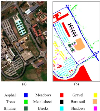
Experiments are performed using the Pavia University data set. This data set was acquired by the ROSIS sensor during a flight campaign in 2003 over the campus of Pavia University in the north of Italy. This data contains 610 by 340 pixels with 103 spectral bands. The geometric resolution is 1.3 m. nine ground-truth classes were considered in the experiments: Trees, Gravel, Meadows, Asphalt, Metal sheets, Bricks, Bitumen, Shadows and Bare soil. Figure 3 shows the ground-truth map and a color composite image of this data set.
(a) (b)
Figure 3. ROSIS hyperspectral dataset over Pavia University used in experiments: (a) colour composition image
(R: 60, G: 30, B: 10). (b) Ground truth map.
To reduce the effects of spectral bands with higher radiance values on those having lower values, the data is linearly normalized in the range of [0, 1]. Furthermore, before using this data sets, its background is ignored. This is because no information is available about these areas.
4.2 Experimental results
In this study, the proposed initialization method for k-means clustering of hyperspectral data is compared with two of most frequently used methods, i.e. Bradley &. Fayyad (BF) and
Estimation the number of endmembers using HFC technique
Estimation spectral signatures of the endmembers using MVES algorithm
random methods. In the first step of the new method, the number of endmembers is estimated by HFC algorithm as 9. The false alarm probability for this detection problem is set to 0.001. As it is said earlier, among different similarity measures for k-means clustering, SSV is used here in all three cases.
In the first case, initial position of cluster centers are obtained using Bradley &. Fayyad (BF) method (Bradley and Fayyad, 1998). According to (Celebi et al., 2013), this method is one of the best methods for k-means initialization in different datasets, and as a result, it is used here to be compared with our proposed method. BF method starts by randomly partitioning of the dataset into J=10 subsets. Clustering results of this case are tabulated in table 1.
Table 1. Confusion matrix based on BF initialization method.
According to table 1, both Gravel and Asphalt classes have not been recognized. That’s why Gravel class has spectral signatures nearly the same as Bricks class on the one hand, and on the other both Asphalt and bitumen have nearly the same spectral signatures. Figure 4 and 5 show these spectral similarities.
Figure 4. Spectral signatures of nine classes in Pavia University Hyperspectral dataset.
Figure 5. Spectral signatures of similar classes in Pavia University Hyperspectral dataset.
In the second case, cluster centers are randomly initialized. Clustering results in this case have been shown in table 2.
Table 2. Confusion matrix based on Random initialization method.
Like the first case, both Gravel and Asphalt classes have not been discriminated in this case. This is because of the above-mentioned reasons.
In the third case, initial position of cluster centers are obtained using MVES method. Clustering results of this case have been shown in table 3.
Table 3. Confusion matrix based on MVES initialization method.
According to table 3, this case leads to highly better results than the other cases. As is obvious, using MVES method not only the best kappa coefficient are obtained but also Asphalt and Bitumen classes are discriminated. For comparative purpose, kappa coefficients and overall accuracies for three cases above are shown in figure 6.
Figure 6. Kappa coefficients and overall accuracies of k-means clustering for different initialization methods.
our proposed method is independent of iterations. In other words, our proposed method leads to the same result in different iterations.
5. CONCLUSION
In order to clustering of hyperspectral data, in this study, a multi-step framework was presented to resolve the problem of initialization of k-means and improve the clustering efficiency. In the first step, HFC is used to estimate the number of endmembers in the image. Then, the spectral signatures of the endmembers are obtained using the MVES algorithm. Lastly, these spectral signatures are used to initialize the k-means clustering algorithm. The proposed method has been compared with two well-known initialization methods, namely, BF and Random methods. Clustering using MVES initialization method with kappa coefficient of 55.3 leads to highly better result than the other two methods. In other words, when MVES’s spectral signatures are used as initial cluster centers, k-means clustering leads to the best result. More importantly, unlike the other two cases, using MVES’s spectral signatures clustering leads to the same results in different iterations, which means, MVES method has the most stability. According to the confusion matrices in all three cases, despite the initial positions of cluster centers, the high spectral similarities of Asphalt and Bitumen classes on the one hand, and Gravel and Bricks classes, on the other, results in deteriorating clustering accuracy. To address last problem, either using another similarity measure or merging these two similar classes can be recommended.
ACKNOWLEDGEMENTS
The authors would like to sincerely thank Tsung-Han Chan, Chong-Yung Chi, Yu-Min Huang, and Wing-Kin Ma, for providing them with MVES Matlab code, and Prof. Gamba (University of Pavia) for sharing the Pavia ROSIS data set.
REFERENCES
Abraham, A., Das, S., Roy, S., 2008. Swarm intelligence algorithms for data clustering, Soft Computing for Knowledge Discovery and Data Mining. Springer, 279-313.
Bradley, P.S., Fayyad, U.M., 1998. Refining Initial Points for K-Means Clustering, ICML. Citeseer, 91-99.
Celebi, M.E., Kingravi, H.A., Vela, P.A., 2013. A comparative study of efficient initialization methods for the k-means clustering algorithm. Expert Systems with Applications 40, 200-210.
Chan, T.-H., Chi, C.-Y., Huang, Y.-M., Ma, W.-K., 2009. A convex analysis-based minimum-volume enclosing simplex algorithm for hyperspectral unmixing. Signal Processing, IEEE Transactions on 57, 4418-4432.
Chein, I.C., Qian, D., 2004. Estimation of number of spectrally distinct signal sources in hyperspectral imagery. Geoscience and Remote Sensing, IEEE Transactions on 42, 608-619.
Craig, M.D., 1994. Minimum-volume transforms for remotely sensed data. Geoscience and Remote Sensing, IEEE Transactions on 32, 542-552.
Farifteh, J., Van Der Meer, F., Carranza, E., 2007. Similarity measures for spectral discrimination of salt‐affected soils. International Journal of Remote Sensing 28, 5273-5293.
Harsanyi, J., Farrand, W., Chang, C., 1993. Determining the number and identity of spectral endmembers: An integrated approach using Neyman-Pearson eigen-thresholding and iterative constrained RMS error minimization.
ENVIRONMENTAL RESEARCH INSTITUTE OF
MICHIGAN, 395-395.
Heinz, D.C., Chein, I.C., 2001. Fully constrained least squares linear spectral mixture analysis method for material quantification in hyperspectral imagery. Geoscience and Remote Sensing, IEEE Transactions on 39, 529-545.
Homayouni, S., Roux, M., 2004. Hyperspectral image analysis for material mapping using spectral matching, ISPRS Congress Proceedings.
Jain, A.K., 2010. Data clustering: 50 years beyond K-means. Pattern Recognition Letters 31, 651-666.
MacQueen, J., 1967. Some methods for classification and analysis of multivariate observations, Proceedings of the fifth Berkeley symposium on mathematical statistics and probability. California, USA, 281-297.
Melgani, F., Pasolli, E., 2013. Multiobjective PSO for Hyperspectral Image Clustering, Computational Intelligence in Image Processing. Springer, 265-280.
Namin, S.R., Naeini, A.A., Samadzadegan, F., 2013. Evaluating the Potential of Particle Swarm Optimization for Hyperspectral Image Clustering in Minimum Noise Fraction Feature Space, Computational Intelligence and Decision Making. Springer, 69-79.
Sun, X., Yang, L., Zhang, B., Gao, L., Zhang, L., 2013. Hyperspectral image clustering method based on Artificial Bee Colony algorithm, Advanced Computational Intelligence (ICACI), 2013 Sixth International Conference on. IEEE, 106-109.
Wagstaff, K., Cardie, C., Rogers, S., Schrödl, S., 2001. Constrained k-means clustering with background knowledge, ICML, 577-584.