FUNDAC¸ ˜AO GETULIO VARGAS ESCOLA DE ECONOMIA DE S ˜AO PAULO
MARCELA MELLO
SHOULD WE WORRY ABOUT THE OBSERVER EFFECT?
EVIDENCE FROM PELOTAS
MARCELA MELLO
SHOULD WE WORRY ABOUT THE OBSERVER EFFECT?
EVIDENCE FROM PELOTAS
Dissertac¸˜ao apresentada `a Escola de Economia de S˜ao Paulo da Fundac¸˜ao Getulio Vargas como requisito para obtenc¸˜ao do t´ıtulo de Mestre em Economia de Empresas
Campo de Conhecimento: Microeconomia
Orientador: Prof. Dr. Bruno Ferman
Mello, Marcela.
Should we worry about the observer effect? Evidence from Pelotas / Marcela Mello - 2016
30f.
Orientador: Bruno Ferman
Dissertação (mestrado) - Escola de Economia de São Paulo.
1. Pelotas (RS). 2. Comportamento - Avaliação. 3. Atitude (Psicologia) - Mudança. 4. Comportamento humano. 5. Educação. I. Ferman, Bruno. II. Dissertação (mestrado) - Escola de Economia de São Paulo. III. Título.
MARCELA MELLO
SHOULD WE WORRY ABOUT THE OBSERVER EFFECT?
EVIDENCE FROM PELOTAS
Dissertac¸˜ao apresentada `a Escola de Economia de S˜ao Paulo da Fundac¸˜ao Getulio Vargas como requisito para obtenc¸˜ao do t´ıtulo de Mestre em Economia de Empresas
Campo de Conhecimento: Microeconomia
Data de aprovac¸˜ao
/ /
Banca Examinadora:
Prof. Dr. Bruno Ferman (Orientador) FGV-EESP
Prof. Dr. Rodrigo Soares FGV-EESP
ABSTRACT
Most social sciences and medical studies assume that being observed does not affect subjects’ behavior. However, interviews may cause changes in individuals’ behavior or may inhibit changes which would occur if they were not being observed. If being observed changes the behavior of the studied population, the sample ceases to be representative of the population. In this paper, I investigate whether individuals periodically interviewed in a longitudinal epidemiological research conducted in Pelotas, Brazil, are affected along relevant dimensions, in particular, education and health. I find only a significant effect on ENEM score.
RESUMO
Grande parte dos estudos em ciˆencias sociais assume que ser observado n˜ao afeta o comportamento dos indiv´ıduos. No entanto, entrevistas podem causar mudanc¸as no comportamento dos indiv´ıduos que n˜ao ocorreriam se eles n˜ao tivessem sido observados. Se ser observado muda o comportamento da populac¸˜ao estudada, ela pode deixar de ser representativa da populac¸˜ao como um todo. Neste trabalho, investiga-se se indiv´ıduos periodicamente entrevistados em uma pesquisa epidemiol´ogica conduzida em Pelotas, Brasil, s˜ao afetados em dimens˜oes relevantes, em particular, educac¸˜ao e sa´ude. Os resultados mostram um efeito significativo apenas na nota do Enem.
Contents
1 Introduction 6
2 Setup 9
3 Data and Descriptive Analysis 12
4 Methodology 15
4.1 Identification . . . 15
4.2 Inference . . . 16
5 Results 20 5.1 Infant Mortality . . . 20
5.2 Education . . . 21
5.3 Robustness . . . 22
5.4 Multiple Outcomes . . . 23
6 Concerns 25 6.1 Peer Effects . . . 25
6.2 Migration . . . 25
7 Conclusion 26
6
1 Introduction
Most social sciences studies assume that being observed does not affect subjects’ behavior. However, interaction with researchers may cause changes in individuals’ behavior or may inhibit changes that would occur if they were not being observed. The mere asking of questions has po-tential to change subsequent behavior, having methodological implications for these studies since it is not possible to separate these changes from what would be the natural behavior of these indi-viduals. If being observed changes the behavior of the studied population, the sample ceases to be representative of the population. Furthermore, it is possible that this observer effect interacts with an experimental intervention, compromising internal validity Zwane et al. (2011). For example, imagine a experiment that tries to incentivize adoption of a certain behavior, say, hand washing, by instructing about its benefits. The investigator organizes a survey that asks about hygiene habits. If the survey reinforces the importance of hand washing, i.e., it is complementary to the treatment, it might overestimate the effect, in comparison to the case in which there is an intervention without a survey. On the other hand, if the observer effect is a substitute to the treatment, the investigator will underestimate the treatment effect.
In this paper, I investigate whether individuals periodically interviewed in a longitudinal epi-demiological research conducted in Pelotas, Brazil, are affected along relevant dimensions, in par-ticular, education and health. I use a study that started in 1982 and follows all individuals born in the municipality of Pelotas on 1982, 1993, 2004 and 2015 from their birth until now and consists on the application of questionnaires and general physical measurements. I analyze whether the par-ticipants of this study had their outcomes changed on infant mortality, drop-out rate, highest grade attended and high school test scores. The survey may have an effect on these outcomes through different channels. The infant mortality rate may be affected because the survey helps mothers to keep up with general health indicators of their children whereas the education outcomes may be affected through questions about participants’ intentions for the future.
Chapter 1. Introduction 7
a higher proportion of these participants made a purchase within the next 6 months when compared with the control group. Spangenberg (1997) asked health club members to predict their frequency in the club and found that members increased their attendance up to six months after they being asked.
Another kind of observer effect is known as Hawthorne effect. It occurs when subjects change their behavior in response of the awareness of being observed. Zwane et al. (2011) investigate whether being surveyed has an effect on health status through an experiment in which Kenya’s households received a water purification solution. In their experiment, they give all participants a water purifier, but only part of them receive a surveyor at home who tests the amount of purifier contained in the water storage. Since people knew the surveyor would check if they used the solu-tion or not, their behavior might be affected. The results show that diarrhea incidence was smaller in households more frequently surveyed.
Surveys also can affect behavior by making some options more salient. Classic economic the-ory assumes individuals consider all options in their choice set. However, individuals have limited attention (Kahneman (2003)). A survey can call individuals’ attention to some options that they would not consider. Zwane et al. (2011) conducted four experiments to investigate whether sur-veys that make neglected options more salient increase the demand for a product in the context of microfinance, finding null results.
In some contexts, behavior can be changed by interaction between surveyors and participants. In the Pelotas’ study, for example, children undergo physical health measurements and mothers are asked about how they take care of their children. So, the interviews can work as medical attention, because mothers might keep up with their children’s health indicators or talk with other participants or surveyors about children’s health. Finally, surveys can impact behavior as a side effect of partic-ipation incentives. If individuals receive money to answer the survey, their income will be affected. This is unlikely to produce sizable effects in the case.
Although we can specify the several channels through which the observer effect can occur, my identification strategy does not allow disentangle these effects. Nonetheless, we can speculate what are the most probable channels in each case. Anyhow, I estimate the aggregated effect, that can provide some evidence about the importance of this effect. Moreover, it is important to stress there are very few studies that try to estimate this effect in the literature.
Chapter 1. Introduction 8
administrative data. I find only a significant effect on ENEM score.
9
2 Setup
I analyze a survey conducted in Pelotas, Brazil, this study follows all individuals born in the city of Pelotas on specific years and applies questionnaires and general physical measurements. Its main objective is to investigate whether early life characteristics, such as birthweight and breastfeeding practices, are associated with adolescent and adult outcomes.
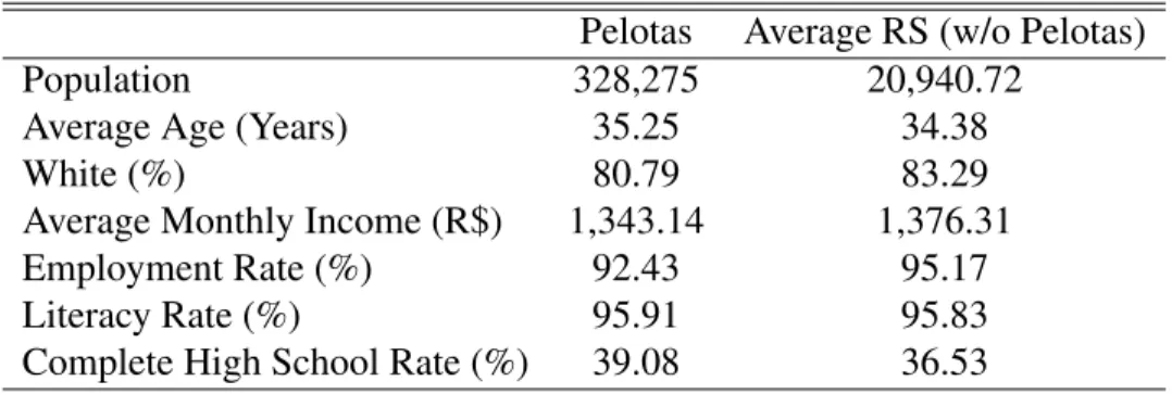
Pelotas is a municipality situated in Rio Grande do Sul (RS), southern Brazil, with a popula-tion of 328,275 inhabitants, the third largest in the state. Table 1 compares Pelotas with RS state. Pelotas’ population is slightly older than the other municipalities and the proportion of whites is smaller than the state’s average, but is still much larger than Brazil’s average (47.7%). The aver-age monthly income and the employment rate are smaller than the state’s averaver-age, however, the education indicators are better than the other municipalities. Note that these differences1 do not necessarily compromise my method, as I rely on a differences-in-differences estimator. These dif-ferences are controlled by the municipality fixed effects.
Table 1: Pelotas and RS Characteristics - 2010 Census
Pelotas Average RS (w/o Pelotas)
Population 328,275 20,940.72
Average Age (Years) 35.25 34.38
White (%) 80.79 83.29
Average Monthly Income (R$) 1,343.14 1,376.31
Employment Rate (%) 92.43 95.17
Literacy Rate (%) 95.91 95.83
Complete High School Rate (%) 39.08 36.53
Note: (i) Average Monthly Income is the average of the income of all jobs, restricted to people 10 years old or more and with positive income. (ii) Employment Rate is the proportion of people 10 years old or more who employed in the reference week. (iii) Literacy Rate includes only people 10 years old or more. (iv) Complete High School Rate includes only people 18 years old or more.
All children born in Pelotas in 1982, 1993, 2004 and 2015 with birth weight above 500g were eligible for the study. To find all children born on the selected years, the surveyors checked all ma-ternity hospitals for deliveries daily. If the mother was in the hospital, they applied a questionnaire and took general physical measurements of the child. If she had already left, they got her address
Chapter 2. Setup 10
in the hospital and conducted the survey at home. The number of children/mothers interviewed in all years is very close to official data in 2004 (93,6%)2.
The follow-up interviews were conducted in different moments for each cohort. The 1993 co-hort, for example, had a special focus on the first year of life for low birth weight children3. While the 1982 and 2004 cohorts were interviewed once and twice, respectively, the 1993 cohort was interviewed four times. For some interviews, all participants are surveyed, while, for others, only a sample of the eligible population is interviewed. I detail the frequency and periodicity of the interviews and the population of each cohort on Table 2.
The surveyors also take participants’ physical measurements, such as weight, height, abnominal circumference, blood pressure etc. The process of data collection is very organized and uses high quality equipment. In 2010, 6-7 years follow-up of 2004 cohort, the average time of an interview was about three hours4. Although participation in the study is voluntary (participants only receive some money5, snacks and transport reimbursement), the attrition rate is very low in all survey years. There is an effort to find participants who migrated from Pelotas6. Table 2 shows the follow-up rate of each cohort and interview. In each interview, the surveyors apply questionnaires to the mother or the child, asking about the child’s literacy, physical activities, feeding, sleeping, health spending, the mother’s health, whether mother or father smoked during pregnancy etc. Obviously, the questions vary according to child’s age Marco and Zanini (2010).
2Birth data in 1993 is not available at SISNAC-DATASUS. 3Low birth weight is defined as less than 2,500 g.
4In the 18-year follow-up questionnaire, there were more than 400 questions.
5In the last interview, participants received R$ 50,00 (US$ 12.50 and approximately 4% of Pelotas’ average income)
to answer the survey.
Chapter 2. Setup 11
Table 2: Interviews and Follow-up Rate
Interview Sample Eligible (N) Follow-up (%)
1993 Cohort
Birth All 1993 births 5,249
-1 month 13% of all cohort members 655 99.1
3 months 13% of all cohort members 655 98.3
6 months Low birthweight children + 20% of others 1,460 96.8 12 months Low birthweight children + 20% of others 1,460 93.4 4 years Low birthweight children + 20% of others 1,460 87.2
11 years All cohort members 5,249 84.8
15 years All cohort members 5,249 82.9
18 years All cohort members 5,249 78.2
2004 Cohort
Birth All cohort members 4,231
-3 months All cohort members 4,231 95.7
1 year All cohort members 4,231 94.3
2 years All cohort members 4,231 93.5
4 years All cohort members 4,231 92.0
6-7 years All cohort members 4,231 90.2
12
3 Data and Descriptive Analysis
I use data from several administrative sources in order to analyze the various potential impacts the observer effect may have on health and education. I do not use data from the Pelotas’ study, because it does not provide information about the non-surveyed individuals, which is crucial to my analysis.
To access the health dimension, I look at the infant mortality rate. The data on deaths comes from SIM-SUS (System of Infant Mortality - Unified Health System). This database consists on in-formation about all children who died before completing one year of age and includes child‘s date of birth and death, place of birth, place where the mother lives, cause of death and other mother and father‘s socioeconomic information1, such as race, parents‘ highest grade attended and income. I identify the children who belong to the treatment group through their birth year and municipality where the mother lives. To construct the infant mortality rate (number of deaths by 1,000 births), I also need the total number of deliveries. The data on births comes from SISNAC-SUS (System of Information of Live Births), which registers information about all births since 1994 and reports children’s date and place of birth, place where the mother lives and socioeconomic information2. Since I do not have data on births for years before 1994, I use information from other years to calculate the mortality rate. The non-availability of data for all years has as consequence the losing of particular variations on births and this problem is especially worse for small cities, which are subjected to stronger variations. For the cohorts between 1991 and 1995, I use the average number of births in 1996 and 1997 because the data before 1996 is unreliable. The choice of using this aver-age instead of the real number introduces another source of variation on my data set. For example, this average is higher than the real value, i.e, if the number of birth is in an increasing trend, the mortality rate will be underestimated. This means the measurement error will be correlated with non-observables. However, we do not expect it to be important if trends are not too strong. One way to access the likely importance of this source of bias, I use an alternative approach that is less likely to be affected. Since the results are similar, I conclude there is no reason for concern.
The alternative approach is using the total population as the denominator of the mortality rate. Population data is available only for 1991 and 1996. I only use population in 1996 because there is information on a larger set of municipalities. This approach also leads to a loss of particular variations on births, but has the advantage of being less volatile over time. Then, there is no addition
Chapter 3. Data and Descriptive Analysis 13
of noise variations. I do the analysis using both measures of infant mortality rate. My preference for the former alternative (average of births) is mainly because this is usual metric in the literature. For the 2004 cohort, since I have the birth data of each year, I use only the number of births as denominator.
I restrict my analysis to deaths that occurred after the second interview. Since the first interview does not provide mothers more information about their children‘s health than they get from the hospital and information is the most probable channel this effect, including deaths that happened between the birth (or the first interview) and the second interview would only add noise.
To estimate the effect on education, I look at dropout rate at age 18, highest completed grade by age 18 and ENEM scores3. I construct the dropout variable using School Census information. I first identify all students enrolled in school in 2007 (first School Census with individual-level data) who were born between 1991 and 1995. Then, I checked whether they were still enrolled in each year of School Census until they complete 18 years old or finish high school. The dropout variable assumes value one if the student left school before completing high school and zero otherwise. Due to computing limitations, this procedure was done separately for each state, which implies that, if a student migrates to other state, I will not be able to follow him anymore and he will be considered as being a dropout even if he is enrolled in a school in other state. This problem would be severe if migration inter-states were large. Using 2010 Census data, only about 3.5% of the population between 14 and 18 years old born in RS left the state.
The highest completed grade by age 18 variable is also constructed using School Census. As in the construction of dropout variable, I first identify all students enrolled in school in 2007 who were born between 1991 and 1995. Then, I identify in which grade they were enrolled when they were 18 years old or the last grade they completed before they dropped out. The variable equals the last grade completed, in years, and has the same problem as the dropout rate regarding to migration. Since I can identify in School Census where students were born and where they live, I exclude students who were born in Pelotas but do not live there anymore (17%). I also exclude students who were not born in Pelotas but live there (13%)4.
Finally, I analyze the effect of being observed on ENEM scores. I compare students’ scores in the four areas of knowledge that the exam covers - Math (MAT), Language (LG), Human Sciences (HS) and Nature Sciences (NS) - and the average score. Both analysis are restricted to 18 years old students who were concluding high school in the year of the exam. The first restriction is due to data constraints: the members of 1991 cohort are 18 years old in 2009, which is the first
3ENEM - National Evaluation of High School. The test is taken by students in the last grade of high school of both
public and private systems. ENEM score is used by many universities as criterion of admission.
Chapter 3. Data and Descriptive Analysis 14
year data is comparable 5, and the members of 1995 cohort are 18 years old in 2013, the last year ENEM’s microdata are available. Hence, 18 years old is the unique age for which there is data for all five cohorts. As explained in the Methodology section, I need balanced cohorts for my identification. Moreover, I include only students who were completing high school, because the test is high stakes for these students. Although this is a selected sample, the results are interned valid for this population. I cannot extend the results to the population of ENEM participants.
Table 3 shows the average of each outcome for the two-year period before (pre-) and after (post-) the treated year for both control and treatment. The last column shows the difference in differences test, using the inference procedure explained in the Methodology section.
Table 3: Outcomes For Not Treated Years (Pre- and Post-) - Treated and Control Units
Pelotas Avg. RS
Pre- Post- Diff Pre- Post- Diff Diff-Diff Infant Mortality 1993 8.99 10.36 1.37 8.20 8.14 -0.06 −1.43
[0.52] Infant Mortality 2004 3.83 2.88 -0.95 3.56 2.34 -1.22 −0.28
[0.64] Highest Grade 1993 8.98 8.35 -0.63 9.46 9.00 -0.46 −0.17
[0.34] Dropout Rate 1993 0.24 0.28 0.04 0.26 0.33 0.07 −0.04
[0.31] Enem Avg. 1993 528.76 503.87 -24.89 521.47 497.12 -24.35 −0.54
[0.90] Enem MAT 1993 525.42 520.80 -4.62 520.61 516.51 -4.09 −0.51
[0.71] Enem LG 1993 536.15 501.90 -34.25 520.94 489.51 -31.43 −2.80
[0.84] Enem NS 1993 517.02 475.92 -41.10 514.28 471.26 -43.02 1.92
[0.99] Enem HS 1993 536.43 516.84 -19.59 530.12 511.29 -18.83 −0.75
[0.92]
Note: (i) p-value in brackets. (ii) *** 1% level of significance; ** 5% level of significance; * 10% level of significance. (iii) For infant mortality, only deaths that occurred after the second interview were con-sidered, i.e., 30 days for 1993 cohort and 90 days for 2004 cohort.
5Since ENEM test changed its format as well as its difficulty in 2009, the scores before and after 2009 are not
15
4 Methodology
4.1
Identification
I estimate the observer effect using a difference-in-difference model1. I estimate the following equation:
Yjt =α·djt+δj +γt+ηjt, (1) where j is the municipality index, t is the cohort index, Yjt is the outcome, djt is the treatment dummy (Pelotas×Treated Cohort),δj is the municipality fixed effect,γtis the cohort fixed effect
andηjtis the random error. This model is estimated separately for 1993 and 2004 cohorts.
My group of comparison consists of all municipalities in RS for which there is available data for the treatment year, two years before and after the treated year for each outcome. For each group of outcomes i.e., education and health, I use the largest number of municipalities for which data is available for every year. I choose RS state as my control group because municipalities in RS share similar demographic and cultural characteristics and mainly because most educational and health policies are taken at the state level, for which I control using time fixed effects (γt).
Note that my design is robust to different linear tendencies between treatment and control groups. This is because I have a single treatment period and an equal number of pre- and post-treatment control years. For example, if the treated group has steeper increasing tendency than the control group, treatment effect will be overestimated if the treatment period is in the later periods, underestimated if it is in the earlier periods, but unbiased if exactly in the middle.
Here, I explicit the hypothesis I need to identify the parameter of interest:
E[YP elotas,t∗(0)]−
E[YP elotas,t∗−1+YP elotas,t∗−2]
4 +
E[YP elotas,t∗+1+YP elotas,t∗+2]
4
=
E[YControl,t∗]−
E[YControl,t∗−1+YControl,t∗−2]
4 +
E[YControl,t∗+1+YControl,t∗+2]
4
,
1Although Synthetic Control Model could also be used in this case (one treated unit), it does not perform well
Chapter 4. Methodology 16
whereYP elotas,t∗(0) is the potential outcome of the treated unit if it had not been treated,t∗ is the
treated year. Note that this hypothesis is valid when there are linear tendencies with different slopes if we have the same number of periods before and after the treated year. However, if there are non-linear differing tendencies, the hypothesis is not valid. To test for this, I estimate a placebo regression for each outcome. For infant mortality outcomes, I use the five-year periods after the treated year and assign treatment status to the middle year (treated year plus three). For educational outcomes, I do not have data of five years before or after the treated year: I exclude the treated year and run the placebo using two years before and three years after the treated year and assign treatment status to the middle year (treated year plus one).
4.2
Inference
In my model, described above, the DID estimator is given by the following expression:
ˆ
α= YP elotas,t∗−
1
T −1
T X
t6=t∗
YP elotas,t !
− 1
N
N X
j6=P elotas
Yj,t∗−
1
T −1
T X
t6=t∗
Yj,t !
ˆ
α→(α+γt∗+ηP elotas,t∗ −
1
T −1
T X
t6=t∗
ηP elotas,t−(γt∗)
ˆ
α→α+ηP elotas,t∗− 1
T −1
T X
t6=t∗
ηP elotas,t
| {z }
W
ˆ
α→α+W
Under the hypothesis of random treatment, my parameter of interest,αˆ, is not biased. However, its consistency depends on an arbitrarily large number of both treatment and control units. Since I have only one unit treated, it is not consistent. Intuitively, since we cannot take the average of the random shocks for the treated unit, we are left with the realization ofW in addition to the interest parameter. ThisW has mean zero, but increasing the number of controls does not bring it closer to its mean. Thus, I cannot employ the usual difference-in-differences inference.
Chapter 4. Methodology 17
In each regression, one of the control group municipalities has its treatment status assigned as treated. These placebos can provide information about the error term in our DID estimator,Wˆ. The main assumption of their method is that the error is i.i.d. among municipalities (in particular, homoskedastic). Under this assumption, I can use information of the control group to estimate the empirical distribution of the error for the treated unit. However, in my case, the homoskedastic assumption is especially unreasonable because municipalities have different population sizes.
To better expose this point, I follow closely Ferman and Pinto (2016). Consider the DID model in the individual level:
Yijt=α·dijt+δj +γt+νjt+εijt (2) Here, the error term is decomposed in two parts: a group x time error term (νjt) and an individual-level error term (εijt). In this setting, the errors of individuals in the same group j might be corre-lated, while individuals from different groups are uncorrelated. For simplicity, assume thatεijtare all not correlated andνjt can be unrestrictedly auto-correlated. Aggregating (3) at the group x time level, we obtain the same equation as in (1):
Yjt =α·djt+δj+γt+νjt (3) Note that the error term (νjt) is heteroskedastic across groups j and can be written as:
ηjt =νjt+
1
M(j, t)
MX(j,t)
i=1
εijt
where M(j, t) is the number of observations in group j at time t. Assuming, for simplicity, that
M(j, t)is constant across j and T is fixed:
var(Wj) =var
1
T −1
T X
t6=t∗
ηjt−ηjt∗
!
=var
1
T −1
T X
t6=t∗
νjt−νjt∗ +
1
T −1
T X
t6=t∗
1 Mj Mj X i=1 εijt
−εijt∗
=A+ B
Mj
Chapter 4. Methodology 18
Heteroskedasticity will cause under-rejection of the null hypothesis when the treated unit is large relative to the controls, as it is in the present case. This under-rejection will happen because the aggregate variance of the treated unit is in fact smaller then what would be estimated using information from the control group.
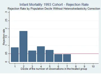
To illustrate this point, I do the following exercise2. First, I exclude Pelotas from the analysis. Then, I do the inference using the Conley and Taber (2011) method switching which municipality will be assigned as treated and I calculate the rejection rate at 5% for each decile of the number of observations in the treated group. Figure 1 shows the result of this exercise using the infant mortality outcome for 1993 cohort. Note that the rejection rate is higher when the treated municipality has a small number of observations compared to the controls and falls considerably when the treated municipality is relatively large. Since Pelotas is one of the largest municipalities in RS, Conley and Taber (2011) method could lead me to not reject the null hypothesis even in the presence of an effect.
Figure 1: Rejection Rate
In order to account to the heteroskedasticity problem, Ferman and Pinto (2016) developed a correction for Conley and Taber (2011) method. They propose to rescale the estimated redisu-als for each municipality according to its population size. Note that, in my case, the source of heteroskedasticity is known. Since my outcome variables are population averages, the error term variance will be approximately inversely proportional to population size.
Ferman and Pinto (2016)’s method is to estimate the variance ofWjas a function of the number of observations in group j (Mj), and then re-scale the residuals used to estimate the distribution of
WP elotas. Practically speaking, I only need to regress Wˆj 2
on M1
j and a constant, and then use
the predicted value, Gd(M), to normalize the residuals, Wˆj, as follows: W˜j = ˆWj r
d
G(MP elotas) d
G(Mj)
.
Chapter 4. Methodology 19
Finally, they suggest the application of a wild cluster bootstrap to their method in order to correct for few number of clusters. The wild cluster bootstrap procedure generates a smoother bootstrap distribution. For each group j, resample with replacementW˜j with probability 0.5 or −W˜j with probability 0.5 N times. Then, calculateαˆb = ˜WP elotas− N1−1
PN
j6=P elotasW˜j. H0 will be rejected ifα <ˆ αˆb(a/2)orα >ˆ αˆb(a−a/2).
Figure 2 shows the same exercise as before, but with Ferman and Pinto (2016) correction. Note that with this correction the rejection rate is much less sensitive to the number of observations than in Conley and Taber (2011) method.
20
5 Results
5.1
Infant Mortality
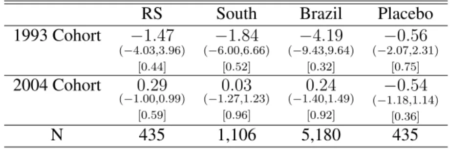
I analyze the effect of being observed on post-neonatal infant mortality. I expect to find a reduc-tion on the infant mortality because, in each interview, surveyors take children physical measure-ments such as weight and height, which might help mothers keep up with general health indicators of their children. In other words, the survey might serve as a medical appointment. Thus, the mostly probable channel behind this effect is social interaction.
This outcome is specially important for 1993 cohort because the researchers focused on low birth weight children who underwent additional interviews. There were four interviews during this period while the 2004 cohort was interviewed once. However, it is important to highlight that not all children were visited every time in their first year of life. Only 13% of the eligible children received the first two follow-up visits and all low birth weight children plus 20% of the others received the next two visits (Table 2). Since I cannot identify these children, I assign treatment status to all the eligible. This assignment might bias my estimates toward zero. We are less likely to find an effect on the 2004’s cohort, first, because there was only one follow-up visit between birth and year one, second, because the infant mortality rate at this time was already low (see Table 3).
Chapter 5. Results 21
to the middle year (treated year plus three). The results show that we cannot reject that tenden-cies are linear on both cohorts. Table 8 reports the results for 1993 cohort using the population as denominator. This alternative approach gives similar results.
Table 4: Infant Mortality
RS South Brazil Placebo
1993 Cohort −1.47
(−4.03,3.96) [0.44]
−1.84
(−6.00,6.66) [0.52]
−4.19
(−9.43,9.64) [0.32]
−0.56
(−2.07,2.31) [0.75] 2004 Cohort 0.29
(−1.00,0.99) [0.59]
0.03
(−1.27,1.23) [0.96]
0.24
(−1.40,1.49) [0.92]
−0.54
(−1.18,1.14) [0.36]
N 435 1,106 5,180 435
Note: (i) Non rejection region is in parenthesis. (ii) p-value in brackets. (iii) *** 1% level of significance; ** 5% level of significance; * 10% level of significance.
5.2
Education
In order to analyze the education dimension, I look at dropout rate at 18 years-old, highest grade attended by 18 years-old students and ENEM scores. I argue that the mostly probable channel behind the effect on education is salience. The questionnaire involves a range of questions about education and also asks about participants’ plans for the future. For example, the questionnaire asks whether the participant is enrolled in school. If she/he is not, it asks why. The questionnaire also asks whether the participant intends to go to university, do a vocational course or work.
Chapter 5. Results 22
Table 5: Highest Grade Attended and Dropout Rate
RS South Brazil Placebo
Highest Grade 0.06
(−0.14,0.12) [0.44]
0.03
(−0.15,0.13) [0.76]
−0.01
(−0.17,0.14) [0.91]
−0.00
(−0.14,0.15) [0.91] Dropout −0.02
(−0.03,0.03) [0.25]
−0.02
(−0.03,0.03) [0.23]
−0.02
(−0.03,0.03) [0.27]
−0.02
(−0.04,0.04) [0.29]
N 444 1,071 5,196 444
Note: (i) Non rejection region is in parenthesis. (ii) p-value in brackets. (iii) *** 1% level of significance; ** 5% level of significance; * 10% level of significance.
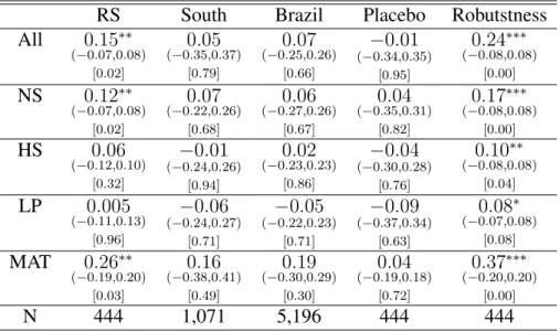
Table 6: Enem Score
RS South Brazil Placebo Robutstness
All 0.15∗∗ (−0.07,0.08)
[0.02]
0.05
(−0.35,0.37) [0.79]
0.07
(−0.25,0.26) [0.66]
−0.01
(−0.34,0.35) [0.95]
0.24∗∗∗ (−0.08,0.08)
[0.00] NS 0.12∗∗
(−0.07,0.08) [0.02]
0.07
(−0.22,0.26) [0.68]
0.06
(−0.27,0.26) [0.67]
0.04
(−0.35,0.31) [0.82]
0.17∗∗∗ (−0.08,0.08)
[0.00] HS 0.06
(−0.12,0.10) [0.32]
−0.01
(−0.24,0.26) [0.94]
0.02
(−0.23,0.23) [0.86]
−0.04
(−0.30,0.28) [0.76]
0.10∗∗ (−0.08,0.08)
[0.04] LP 0.005
(−0.11,0.13) [0.96]
−0.06
(−0.24,0.27) [0.71]
−0.05
(−0.22,0.23) [0.71]
−0.09
(−0.37,0.34) [0.63]
0.08∗ (−0.07,0.08)
[0.08] MAT 0.26∗∗
(−0.19,0.20) [0.03]
0.16
(−0.38,0.41) [0.49]
0.19
(−0.30,0.29) [0.30]
0.04
(−0.19,0.18) [0.72]
0.37∗∗∗ (−0.20,0.20)
[0.00]
N 444 1,071 5,196 444 444
Note: (i) Non rejection region is in parenthesis. (ii) p-value in the second bracket. (iii) *** 1% level of significance; ** 5% level of significance; * 10% level of significance.
year and run the placebo using two years before and three years after the treated year and assign treatment status to the middle year (treated year plus one). I do not reject the tendencies are linear.
5.3
Robustness
Chapter 5. Results 23
heterogeneity that we cannot control for with fixed effects, the dispersion of the residuals with be very large.
One possible source of heterogeneity is that there are different non-linear tendencies across states. I test for this possibility through the following regression:
Ysjt =αt+βj +γs·States·t+δs·State×D1993+εsjt
where s is the state index, j is the municipality index, t is the cohort index,Yjt is the outcome,αj is the cohort fixed effect,βj is the municipality fixed effect,γsis the state specific linear tendency,δs is the statesinteracted with a dummy for 1993 cohort, andηsjt is the random error. This model is estimated excluding Pelotas and using RS as base-group.
Table 9 in the Appendix reports the coefficient of each statesinteracted with a dummy for 1993 cohort (δs) for ENEM score. Since many coefficients are significant and they are jointly significant, we can conclude that there are different non-linear tendencies across states. Thus, South1and Brazil are not good controls for Pelotas.
5.4
Multiple Outcomes
Since I am testing several outcomes, I correct my inference procedure for multiple testing fol-lowing Anderson (2012) approach. I construct two summary index, one for education and the other for health. Testing summary index instead of individual outcomes has the advantage of being more robust to overtesting, because each index represents only a single test. So, the addition of out-comes does not increase the probability of a false rejection. Moreover, the summary index indicates whether there exists a ”general effect”, making interpretation easier. Finally, to construct the sum-mary index, more information is used, what makes this test more powerful than individual-level tests.
The idea of the summary index is to average the standardized outcomes weighted by the inverse of the covariance matrix. Here, I explicit the calculation of the summary index:
sij = (1’Σˆ−j11)
−1(1’Σˆ−1 j y˜ij),
where i is an individual and j is a group (in my case: education or health), y˜ij is the outcome in group j divided by the standard deviation of the control group and corrected to be in the ”best
1Region South is composed by three states: Rio Grande do Sul (RS), Santa Catarina (SC) and Paran´a (PR). Note
Chapter 5. Results 24
direction”,1is a column vector of ones andΣˆ−1
j is the inverted covariance matrix for group j. After calculating this index, I use the inference procedure described in the Methodology section.
Table 7 shows the results of the multiple testing. For both education and health index, I find they are in the direction of improving results. I find a 10% significant effect for the education index. As in the other results, the inclusion of more units of control leads to a loss of precision, but these control units are not good controls.
Table 7: Multiple Testing - Summary Index Treatment South Brazil Placebo
Health
0.09
(−0.53,0.54) [0.77]
0.12
(−0.51,0.53) [0.67]
0.05
(0.50,0.47) [0.76]
0.28
(−0.34,0.36) [0.22]
N 435 1,106 5,331 435
Education
0.19∗ (−0.18,0.17)
[0.08]
0.08
(−0.30,0.29) [0.63]
0.08
(−0.32,0.31) [0.64]
0.07
(−0.29,0.27) [0.65]
N 444 1,071 5,178 444
25
6 Concerns
6.1
Peer Effects
A possible concern about the identification is that the mothers of treated children might use the knowledge they learned in the interviews to benefit their other children. In this case, I may have attributed the non treatment status to treated individuals, which could bias my estimates toward zero. It would be a problem if the proportion of individuals who have siblings whose age difference was equal or inferior to two years was high. I checked in the 2010 Census this proportion and I verified that only 20% of people had siblings with an age difference of two years or less. So, it does not seem to be a first order concern.
6.2
Migration
26
7 Conclusion
This paper investigates whether individuals periodically observed can be affected along relevant dimensions, in particular, education and health. To address this question, I use a study that started in 1982 and follows all individuals born in Pelotas on 1982, 1993, 2004 and 2015 from their birth until now and consists on the application of questionnaires and general physical measurements. To identify the observer effect, I employ a difference-in-differences strategy, comparing the treated co-horts with the adjacent coco-horts and with other municipalities and use recently developed inference methods to account for a small number of treated units.
The results show that there was not any effect on infant mortality rate for either 1993 and 2004 cohorts, but it is important to remember that this may be because of lack of statistical power. In the education dimension, the point estimate of all outcomes are in the direction of improving results. Only ENEM test scores were significantly affected but, as was presented, I cannot include other municipalities to test for it robustness.
27
Bibliography
Abadie, A., Diamond, A., and Hainmueller, J. (2015). Comparative politics and the synthetic control method. American Journal of Political Science, 59(2):495–510.
Anderson, M. L. (2012). Multiple inference and gender differences in the effects of early interven-tion: A reevaluation of the abecedarian, perry preschool, and early training projects. Journal of the American statistical Association.
Conley, T. G. and Taber, C. R. (2011). Inference with “difference in differences” with a small number of policy changes. The Review of Economics and Statistics, 93(1):113–125.
Ferman, B. and Pinto, C. (2016). Inference in differences-in-differences with few treated groups and heteroskedasticity. Working Paper.
Kahneman, D. (2003). Maps of bounded rationality: Psychology for behavioral economics. Amer-ican economic review, pages 1449–1475.
Marco, P. and Zanini, R. (2010). Relat´orio trabalho de campo - acompanhamento 6-7 anos. Avail-able on http://www.epidemio-ufpel.org.br/site/content/coorte 2004/questionarios.php.
Morwitz, V. G., Johnson, E., and Schmittlein, D. (1993). Does measuring intent change behavior? Journal of consumer research, pages 46–61.
Sherman, S. J. (1980). On the self-erasing nature of errors of prediction. Journal of personality and Social Psychology, 39(2):211.
Spangenberg, E. (1997). Increasing health club attendance through self-prophecy. Marketing Let-ters, 8(1):23–31.
Victora, C. G., Ara´ujo, C. L. P., Menezes, A. M. B., Hallal, P. C., Vieira, M. d. F., Neutzling, M. B., Gonc¸alves, H., Valle, N. C., Lima, R. C., Anselmi, L., et al. (2006). Methodological aspects of the 1993 pelotas (brazil) birth cohort study. Revista de saude publica, 40(1):39–46.
28
A Tables
Table 8: Infant Mortality - Population
RS South Brazil Placebo
1993 Cohort −2.79
(−7.34,7.09) [0.48]
−3.52
(−9.47,9.41) [0.48]
−7.99
(−17.79,18.89) [0.37]
−1.05
(−4.81,5.19) [0.82]
N 402 1,019 4,904 402
Note: (i) Non rejection region is in parenthesis. (ii) p-value in brackets. (iii) *** 1% level of significance; ** 5% level of significance; * 10% level of significance. (iv) For the 1993 cohort estimations, I use 1996 population as denominator.
Table 9: Test for Non-Linear Tendencies Across States.
(1) (2) (3) (4) (5)
VARIABLES Average Score MAT NS HS LG
RO×D1993 0.0368 0.0180 -0.00260 0.0311 0.0834
(0.0720) (0.0745) (0.0675) (0.0715) (0.0590)
AC×D1993 -0.0201 -0.0285 -0.177** -0.0134 0.154**
(0.0720) (0.0748) (0.0735) (0.0842) (0.0630)
AM×D1993 0.0973 -0.0287 0.0810 0.117* 0.188**
(0.0651) (0.0618) (0.0649) (0.0643) (0.0766)
RR×D1993 0.217*** 0.0884 0.152* 0.198** 0.329***
(0.0746) (0.0545) (0.0787) (0.0851) (0.0844)
PA×D1993 0.0185 0.00890 0.0115 0.0110 0.0344
(0.0584) (0.0455) (0.0616) (0.0627) (0.0573)
AP×D1993 0.134* -0.0213 0.111* 0.189*** 0.205**
(0.0720) (0.0674) (0.0659) (0.0710) (0.0827)
TO×D1993 0.0632 0.00226 0.0668 0.0227 0.141**
(0.0605) (0.0514) (0.0643) (0.0608) (0.0604)
MA×D1993 -0.0435 -0.102** -0.0748 -0.0547 0.100*
(0.0590) (0.0485) (0.0546) (0.0614) (0.0593)
PI×D1993 0.0973 0.117* 0.0674 0.0162 0.132
(0.0875) (0.0606) (0.0743) (0.0937) (0.0916)
Chapter A. Tables 29
(0.0613) (0.0576) (0.0636) (0.0579) (0.0557)
RN×D1993 0.162** 0.0882 0.0746 0.180*** 0.221***
(0.0778) (0.0911) (0.0822) (0.0691) (0.0580)
PB×D1993 0.0443 0.0164 -0.00527 0.0193 0.129**
(0.0613) (0.0558) (0.0641) (0.0629) (0.0584)
PE×D1993 -0.0800 -0.0987** -0.0737 -0.0637 -0.0313
(0.0603) (0.0496) (0.0575) (0.0613) (0.0623)
AL×D1993 0.134* 0.0185 0.0489 0.112 0.304***
(0.0684) (0.0754) (0.0638) (0.0719) (0.0686)
SE×D1993 0.0387 -0.0100 -0.0559 0.0973 0.106*
(0.0579) (0.0594) (0.0612) (0.0596) (0.0584)
BA×D1993 0.0560 -0.00267 0.0375 0.0694 0.0979*
(0.0573) (0.0550) (0.0545) (0.0552) (0.0594)
MG×D1993 0.216*** 0.272*** 0.190*** 0.160*** 0.0973**
(0.0636) (0.0658) (0.0601) (0.0557) (0.0494)
ES×D1993 0.0517 0.0356 0.0423 0.0398 0.0623
(0.0662) (0.0629) (0.0632) (0.0631) (0.0607)
RJ×D1993 0.108* 0.159*** 0.110* 0.0572 0.0328
(0.0606) (0.0488) (0.0633) (0.0696) (0.0595)
SP×D1993 0.0479 0.0404 0.0930* 0.0254 0.00668
(0.0593) (0.0534) (0.0550) (0.0578) (0.0465)
PR×D1993 0.0653 0.0519 0.0365 0.0705 0.0647
(0.0660) (0.0525) (0.0621) (0.0643) (0.0649)
SC×D1993 0.300*** 0.356*** 0.195*** 0.262*** 0.193***
(0.0717) (0.0651) (0.0719) (0.0689) (0.0625)
MS×D1993 -0.0168 0.0593 -0.0376 -0.0576 -0.0346
(0.0912) (0.0727) (0.0869) (0.0865) (0.0834)
MT×D1993 -0.0305 -0.128* 0.00463 0.000376 0.0396
(0.0811) (0.0652) (0.0788) (0.0706) (0.0842)
GO×D1993 0.121** 0.132*** 0.0757 0.0890 0.112**
(0.0583) (0.0508) (0.0588) (0.0573) (0.0542)
DF×D1993 -0.111* -0.0852* -0.0714 -0.0446 -0.188***
(0.0618) (0.0501) (0.0830) (0.0663) (0.0698)
Observations 25,975 25,975 25,975 25,975 25,975
F 4.58 7.15 3.50 3.72 5.40
R-squared 0.934 0.911 0.931 0.926 0.920
Robust standard errors in parentheses