An optimally tuned ensemble of the "eb_go_gs" configuration of GENIE: parameter sensitivity and bifurcations in the Atlantic overturning circulation

(1)

GMDD

6, 925–956, 2013

An optimally tuned GENIE ensemble

R. Marsh et al.

Title Page Abstract Introduction Conclusions References

Tables Figures

◭ ◮

Back Close

Full Screen / Esc

Printer-friendly Version Interactive Discussion

Discussion

P

a

per

|

Dis

cussion

P

a

per

|

Discussion

P

a

per

|

Discussio

n

P

a

per

|

Geosci. Model Dev. Discuss., 6, 925–956, 2013 www.geosci-model-dev-discuss.net/6/925/2013/ doi:10.5194/gmdd-6-925-2013

Geoscientiic Geoscientiic

Geoscientiic

Open Access

Geoscientiic Model Development

Discussions

This discussion paper is/has been under review for the journal Geoscientific Model Development (GMD). Please refer to the corresponding final paper in GMD if available.

An optimally tuned ensemble of the

“eb go gs” configuration of GENIE:

parameter sensitivity and bifurcations

in the Atlantic overturning circulation

R. Marsh1, A. S ´obester2, E. E. Hart2, K. I. C. Oliver1, N. R. Edwards3, and S. J. Cox2

1

National Oceanography Centre Southampton, University of Southampton, Waterfront Campus, European Way, Southampton SO14 3ZH, UK

2

Faculty of Engineering and the Environment, University of Southampton, Southampton SO17 1BJ, UK

3

Department of Earth and Environmental Sciences, CEPSAR, The Open University, Milton Keynes MK7 6AA, UK

Received: 24 August 2012 – Accepted: 27 December 2012 – Published: 11 February 2013

Correspondence to: R. Marsh ([email protected])

(2)

GMDD

6, 925–956, 2013

R. Marsh et al.

Tables Figures

◭ ◮

Back Close

Full Screen / Esc

Discussion

P

a

per

|

Dis

cussion

P

a

per

|

Discussion

P

a

per

|

Discussio

n

P

a

per

|

Abstract

The key physical parameters of the “eb go gs” configuration of GENIE, an Earth sys-tem Model of Intermediate Complexity (EMIC), are tuned using a multi-objective ge-netic algorithm. An ensemble of 90 parameter sets is tuned using two ocean and two atmospheric state variables as targets. These are “Pareto-optimal”, representing 5

a range of trade-offs between the four tuning targets. For the leading five parameter sets, simulations are further evaluated alongside a simulation with untuned “default” parameters, comparing selected variables and diagnostics that describe the state of the atmosphere, ocean and sea ice. One of these parameter sets is selected for fur-ther analysis of the objective function (error) landscape in the vicinity of its tuned values. 10

“Cli_ffs” along some dimensions motivate closer inspection of corresponding variations in the Atlantic meridional overturning circulation (AMOC). This reveals that bifurcations in the AMOC are highly sensitive to parameters that are not commonly associated with MOC stability. Specifically, the state of the AMOC is sensitive to parameters govern-ing the wind-driven circulation and atmospheric heat transport. Five optimal parameter 15

sets are recommended for future use of GENIE in the configuration presented here.

1 Model calibration and parameter space analysis

Earth System models of full complexity are computationally expensive, due to the reso-lution of physical and biogeochemical processes on short time and space scales. Rela-tively small (O(10)-member) ensembles of relaRela-tively short (centennial) simulations are 20

commonplace. Simulations and predictions with such models are nonetheless sensi-tive to the parameters for key unresolved processes, such as turbulent mixing of ocean tracers and cloud physics. The uncertainty due to such parameter sensitivity may be considerable, and is the subject of much ongoing research (Slingo et al., 2009). A range of non-linear behaviour in the Earth system (Lenton et al., 2008) may be likewise 25

(3)

GMDD

6, 925–956, 2013

R. Marsh et al.

Tables Figures

◭ ◮

Back Close

Full Screen / Esc

Discussion

P

a

per

|

Dis

cussion

P

a

per

|

Discussion

P

a

per

|

Discussio

n

P

a

per

|

models. The comparative computational affordability of Earth system models of inter-mediate complexity (EMICs) facilitates quantifying their uncertainties due to mixing and transport parameter choices in particular. Additionally, through carefully designed ex-periments and optimization studies across the space of these parameters, the locations of sub-domains of parameter space within which model behaviour may be regarded as 5

plausible (i.e. neither unphysical nor in unacceptable disagreement with observations) may be identified, yielding insights into these sub-domains and into the optimal com-position of ensembles that best enable the meeting of observational targets. Conse-quently, the dependence of emergent non-linear behaviour on key model parameters may become apparent.

10

One particular family of EMICs is built using the Grid ENabled Integrated Earth sys-tem modelling (GENIE) framework. At the core of many GENIE models is the most basic climate model in which atmosphere, ocean and sea ice all play an active role, configured on a 36×36 equal-area-partitioning of the Earth surface with 16 depth layers

in the ocean. This climate core has been used extensively, in studies of past, present 15

and future Earth System dynamics (Cao et al., 2009). In the present study, we report the results from an objective tuning of the most recently documented version of the basic climate model (Marsh et al., 2011). As such, this paper is the second in a series that document the development, evaluation and benchmarking of GENIE.

Edwards and Marsh (2005) reported an early parameter sensitivity study of 20

C-GOLDSTEIN, the predecessor to GENIE, which has almost identical ocean and climate dynamics in a simpler (although less flexible) computational implementation. They used a semi-random ensemble of 1000 simulations, with which they addressed both the inverse problem of parameter estimation, and the direct problem of quantify-ing the uncertainty due to mixquantify-ing and transport parameters. Subsequent analysis of the 25

(4)

GMDD

6, 925–956, 2013

R. Marsh et al.

Tables Figures

◭ ◮

Back Close

Full Screen / Esc

Discussion

P

a

per

|

Dis

cussion

P

a

per

|

Discussion

P

a

per

|

Discussio

n

P

a

per

|

circulation, presenting itself as a cliff-edge catastrophe in the freshwater forcing dimen-sion of the input space. They also concluded that the exact location of this implausible subspace is a function of several other model parameters.

The identification of plausible sets was also the goal of the study by Holden et al. (2010), with deterministic emulators for five di_fferent aspects of the climate state as the 5

key tool. The plausible ensemble was achieved by building, and then using, a statistical filtering process known as Approximate Bayesian Computation. Emulators appeared in a supporting role in the calibration study by Price et al. (2009), where four observational target sets were selected and a multi-objective, emulator-assisted optimizer was used to identify effective ensembles.

10

Here we use an updated version of GENIE (Marsh et al., 2011) to probe into the structure of the landscapes of four similar targets, related to ocean and atmosphere prognostic variables, in the space of 13 of the GENIE parameters. A goal is to identify a diverse range of parameter sets, each of which provides a di_fferent Pareto-optimal fit to observations representing a different balance of processes, thus providing an ef-15

fective database for testing robustness when inter-model comparisons are not readily available. We discuss a simple evolutionary heuristic for the fast identification of en-sembles that simultaneously optimize these targets, also examining the plausibility of these Pareto-optimal parameter sets through a set of further diagnostics for sea ice and the ocean circulation. One of the five lowest error parameter sets is used to further 20

(5)

GMDD

6, 925–956, 2013

R. Marsh et al.

Tables Figures

◭ ◮

Back Close

Full Screen / Esc

Discussion

P

a

per

|

Dis

cussion

P

a

per

|

Discussion

P

a

per

|

Discussio

n

P

a

per

|

2 The model

The EMIC at the centre of this study is “eb go gs” configuration of GENIE-1, com-prising an energy and moisture balance model (EMBM) for the atmosphere, coupled with the Global Ocean Linear Drag Salt and Temperature Equation Integrator (GOLD-STEIN) 3-D ocean model and a dynamic and thermodynamic sea ice model. This setup 5

largely follows that of Edwards and Marsh (2005), but uses an updated model version as integrated into the GENIE framework as described by Marsh et al. (2011). This ver-sion, based on GENIE version 2.7.4, includes revised wind forcing. Here, we tune the setup referred to as “3636s16l” by Marsh et al. (2011), a standard model resolution with horizontal resolution of equal-area grid cells of 10 degrees longitudinal extent and 10

16 depth levels in the ocean, which has been used for a wide range of studies. In the following sub-sections, the three components of“eb go gs” are outlined briefly.

2.1 Atmosphere

The EMBM represents the atmosphere as a single 2-D layer with an advective-diffusive transport scheme for heat and moisture. The prognostic variables are air temperature 15

and specific humidity, representative of the total atmospheric air column. Planetary albedo and the annual-average wind fields for advective transports are prescribed, while transport and ancillary parameters are typically calibrated using data assimila-tion techniques. Physical processes represented by the model are greatly simplified, examples are the instantaneous return of continental precipitation to coastal ocean 20

points via a runo_ff map or the parameterisation of outgoing long wave radiation by an empirical polynomial function. An implicit numerical scheme is used to allow long EMBM timesteps.

2.2 Ocean

GOLDSTEIN comprises a reduced physics (frictional-geostrophic) 3-D ocean model 25

(6)

mul-GMDD

6, 925–956, 2013

R. Marsh et al.

Tables Figures

◭ ◮

Back Close

Full Screen / Esc

Discussion

P

a

per

|

Dis

cussion

P

a

per

|

Discussion

P

a

per

|

Discussio

n

P

a

per

|

tiple islands, and wind-stress forcing from a prescribed 2-D annual-mean wind-stress forcing field (Edwards and Marsh, 2005; Marsh et al., 2011). The prognostic variables are temperature and salinity. The tracer transport scheme employs an isoneutral and eddy-induced mixing scheme and an efficient convection scheme. Unlike primitive-equation ocean models, momentum advection and acceleration terms are neglected 5

in the equation of motion, allowing the use of timesteps which are long relative to those generally used in 3-D ocean models.

2.3 Sea ice

The third component of“eb go gs” is a dynamic and thermodynamic sea-ice model (Edwards and Marsh, 2005; Marsh et al., 2011) (herein referred to as GS). Sea ice is 10

transported with the surface ocean current and is subject to a diffusive process with a strength controlled by a tunable parameter. An implicit numerical scheme for sea-ice transport is available (Marsh et al., 2011) and is used in this study.

3 Objective targets and tuning method

Table 1 lists the 13 dimensions of the EMBM – GOLDSTEIN – GS parameter space with 15

respect to which we are investigating the model sensitivities. Twelve of these param-eters comprise the set used by Edwards and Marsh (2005). We have added a further atmospheric parameter,r_κ, controlling the reduction of meridional heat diffusion over Antarctica and the Southern Ocean south of 56◦_{S, introduced to parameterise the} par-tial isolation of the atmosphere in this region, reducing atmospheric temperatures in the 20

Southern Hemisphere high latitudes (see Appendix A in the publication by Cao et al., 2009 and also Marsh et al., 2011). Further tunable parameters of the “eb go gs” model have been fixed at their default values for the present study.

Table 2 lists the four observational fields that we use to define the targets of the en-semble selection study. These datasets, denoted byST_ocn,SS_ocn,ST_atm andSQ_dryin what 25

(7)

GMDD

6, 925–956, 2013

R. Marsh et al.

Tables Figures

◭ ◮

Back Close

Full Screen / Esc

Discussion

P

a

per

|

Dis

cussion

P

a

per

|

Discussion

P

a

per

|

Discussio

n

P

a

per

|

and are similar to those used in earlier studies. A notable exception to some earlier studies (e.g. Edwards and Marsh, 2005; Price et al., 2009) includes the replacement of the specific atmospheric humidity with a climatology of relative humidity (for reasons discussed in Lenton et al., 2006 and Marsh et al., 2011). The observational data are aligned with the model grid points through linear interpolation. In the case of the 3-D 5

temperature and salinity fields, some of the values for some grid points of the model ocean are filled with the value of the closest available points from the observational fields.

The root-mean-squared (RMS) errors defined by these fields and corresponding out-put fields from“eb go gs” for the last year of a 5000-yr spin-up model integration (s_T_ocn, 10

sS_ocn,sT_atm andsQ_dry) define fourobjective functions:

fT_ocn(x)=

v u u u u

t 1

NT_ocn NT_ocn

X

i=1 h

s_T

ocn(x)−STocn i2

b

σ2

Socn

, (1)

fS_ocn(x)=

v u u u u

t 1

NS_ocn NS_ocn

X

i=1 h

s_S

ocn(x)−SSocn i2

b

σ_S2

ocn

, (2)

f_T

atm(x)= v u u u u

t_N1

T_atm N_T_atm

X

i=1 h

s_T_atm(x)−STatm i2

b

σ_T2

atm

(8)

GMDD

6, 925–956, 2013

R. Marsh et al.

Tables Figures

◭ ◮

Back Close

Full Screen / Esc

Discussion

P

a

per

|

Dis

cussion

P

a

per

|

Discussion

P

a

per

|

Discussio

n

P

a

per

|

and

fQ_dry(x)=

v u u u u

t_N1

Q_dry N_Q

dry X

i=1 h

s_Q

dry(x)−SQdry i2

b

σ_Q2

dry

, (4)

wherex₌W,κh,κv,λ,κt,κq,βT,βq,Fa,ld,ls,κhi,rκ , and the 13 dimensions of this

vec-tor correspond to the parameters defined in Table 1.

The varianceσc2_{in the four expressions above is designed to weight the root mean}

5

squared error in a way that makes the values of the four functions approximately com-parable. This is the same formulation as used in Price et al. (2009), so the results reported there are directly comparable with ours, except forf_Q_dry, as indicated earlier. With these functions we formulate a multi-objective search, the goal of which is to build ensembles comprisingnon-dominatedparameter sets. Such vectors, also known 10

as Pareto-optimal points of the parameter space, have the property that each

out-performs all other points in the set along one of the four dimensions of the output space.

This methodology builds on earlier tuning work by Edwards and Marsh (2005), who sampled the entire parameter space of the (pre-GENIE) C-GOLDSTEIN model through 15

a semi-random, space-filling sampling plan of 1000 individual simulations, and used the responses of the model as the basis for parameter sensitivity analysis. The drawback of this approach is poor scalability with increased problem dimensionality: the number of runs required for a factorial design increases exponentially with the number of pa-rameters to be tuned, although even simple Latin hypercube designs (such as used by 20

Edwards and Marsh, 2005) are much more efficient.

Multi-objective evolutionary search methods, such as the one adopted here (simi-lar to that used by Price et al., 2009) are more robust to this curse of dimensionality

(9)

GMDD

6, 925–956, 2013

R. Marsh et al.

Tables Figures

◭ ◮

Back Close

Full Screen / Esc

Discussion

P

a

per

|

Dis

cussion

P

a

per

|

Discussion

P

a

per

|

Discussio

n

P

a

per

|

sible regions of the search space through a sequence of generations, during which the selective pressure of the optimizer biases each population towards non-dominated individuals. This will, ultimately, result in a fuller understanding of the tuning landscape than a process that either samples uniformly (Edwards and Marsh, 2005) or considers each target (objective function) in isolation, the latter being prone to the risk of biasing 5

the tuning process towards solutions that excel on individual targets, if model structural error is not properly accounted for. Of course, the genetic multi-objective search comes with no mathematical guarantees of convergence (not even to locally non-dominated parameter sets), but experience shows that this class of heuristics is better suited to problems with high dimensionality, especially those that exhibit discontinuities (which, 10

as we shall see, are a feature of the tuning landscape being considered here).

4 Results

We first address the initial generation of non-dominated ensembles of equilibrium so-lutions and the identification of Pareto fronts in 2-D target space. We then outline the isolation of five equally plausible parameter sets, based on the appraisal of atmospheric 15

and ocean state variables, and three sensitive model diagnostics (2-D fields). Finally, we focus on the sensitivity of the four objective functions and one of these diagnostics to key parameters in the vicinity of one tuned parameter set, exploring features of the “landscape” associated with variations in these parameters.

4.1 Identifying non-dominated ensembles 20

(10)

GMDD

6, 925–956, 2013

R. Marsh et al.

Tables Figures

◭ ◮

Back Close

Full Screen / Esc

Discussion

P

a

per

|

Dis

cussion

P

a

per

|

Discussion

P

a

per

|

Discussio

n

P

a

per

|

continuities caused by AMOC collapse. The particular heuristic adopted here is the Non-dominated Sorting Genetic Algorithm (NSGA-II, Deb et al., 2002).

Given a CPU time of 2 h and 10 min for a model run with a 5000-yr spin-up and the availability of approximately 90 processors at any one time on the University of Southampton Iridis 3 supercomputer, we opted for a population size of 90 individuals, 5

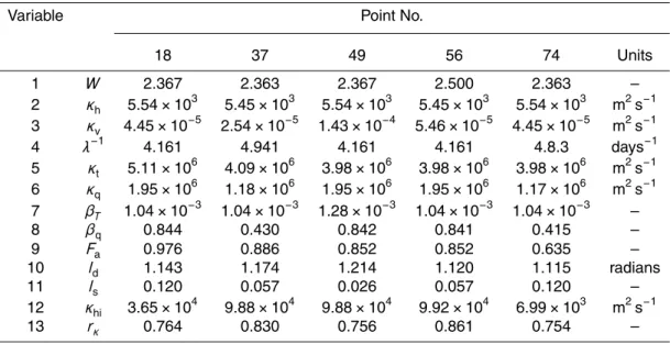
giving a generation wall-clock time of 2 h 10 min. We ran the ensemble selection search over 20 generations – this yielded the Pareto fronts (or, more specifically, 2-D projec-tions of Pareto fronts) depicted in Fig. 1, which illustrates the relaprojec-tionships between objective functions that measure goodness of fit, or model error.

A noteworthy feature of these fronts is thatT_ocn andS_ocn, as well asT_ocn and T_atm, 10

appear to be reasonably well correlated in the region of the best objective values, while the shape of the fronts related to the other possible pairings indicates some level of competition between these objective functions. The former correlations can be inter-preted physically: correlation of theTocn andSocn objective functions is consistent with

obtaining water mass properties, temperature and salinity, that are closest to obser-15

vations; correlation of theTocn andTatm objective functions is consistent with obtaining

a more realistic climate state, as ocean and air temperatures are tightly coupled. The apparent competition between Socn and Qdry in particular may reflect a trade-off

be-tween realism over land or oceans, or bebe-tween climate zones, so more realistic ocean salinity may be obtained with less realistic land humidity, or more realistic low-latitude 20

salinity may be obtained with less realistic high latitude humidity (and vice versa in both cases). Mapping the Pareto front back into the 13-dimensional parameter space yielded the histograms shown on Fig. 2. Clearly some distributions are bimodal, further suggesting trade-offs between different processes/regions and objective functions. 4.2 An ensemble of five parameter sets

25

(11)

GMDD

6, 925–956, 2013

R. Marsh et al.

Tables Figures

◭ ◮

Back Close

Full Screen / Esc

Discussion

P

a

per

|

Dis

cussion

P

a

per

|

Discussion

P

a

per

|

Discussio

n

P

a

per

|

feature in the top third of the overall objective function ranges of the 90 points against all four of their objectives. The values of the input variables for these 5 points are shown in Table 3. For closer examination of these points, and for comparison with the corresponding Marsh et al. (2011) configuration (using untuned parameters, hence-forth GMD11), we evaluate selected variables and diagnostics that describe the state 5

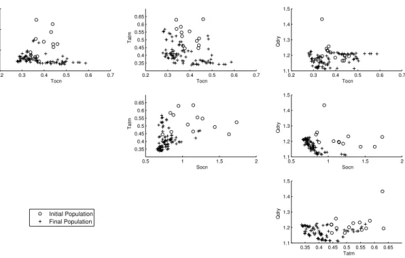
of the atmosphere, ocean and sea ice. Figures S1–12 (Supplement) show simulated, observed and difference (simulated minus observed) fields, for annual-mean surface air temperature and specific humidity (Figs. S1–6), and for annual-mean sea surface temperature and salinity (Figs. S7–12). We show corresponding Taylor diagrams for air temperature (Fig. 3a), specific humidity (Fig. 3b), sea surface temperature (Fig. 3c), 10

sea surface salinity (Fig. 3d), and also for full-depth ocean temperature (Fig. 3e) and salinity (Fig. 3f). Figure 4a through 4e show annual-mean sea ice concentrations and thicknesses for this small ensemble, with Figs. 5a through 5e and 6a through 6e show-ing respectively the barotropic streamfunction and the Atlantic Meridional Overturnshow-ing streamfunction. As a reference, Figs. 4f, 5f and 6f show the sea ice variables and ocean 15

circulation streamfunctions for GMD11.

We first consider the atmosphere (Figs. S1–6). The model is cooler than observa-tions at most locaobserva-tions, with particularly large errors in the Eurasian Arctic. Tropical humidities are generally too high, with the particular exception of anomalously low humidities over the eastern subtropical basins for points 18, 49 and 56. The surface 20

ocean is generally characterised by a cold Atlantic sector and a warm/cold dipole in the west/east Pacific, and largest salinity errors at western boundaries and at high latitudes (Figs. S7–12). Differences between the fits of each simulated property distribution to observations are captured in the Taylor diagrams (Fig. 3), where standard deviations of 1.0 correspond to the correct amplitude of property distribution. Parameter tuning both 25

(12)

GMDD

6, 925–956, 2013

R. Marsh et al.

Tables Figures

◭ ◮

Back Close

Full Screen / Esc

Discussion

P

a

per

|

Dis

cussion

P

a

per

|

Discussion

P

a

per

|

Discussio

n

P

a

per

|

least so for points 37 and 74. For sea surface temperature, only marginal differences arise in standard deviation and correlation for points 37 and 74. For sea surface salin-ity, standard deviation is substantially improved, with reduced correlation, for points 18 and 56. As for surface temperature, the fits of full-depth temperature distributions are little altered by tuning. For full-depth salinity, standard deviation is improved for point 5

18, but standard deviation and correlation are both degraded for points 37, 49 and 74. Beyond property distributions, we also evaluate aspects of the climate system that are of regional importance and likely to play key roles in the transient response to ra-diative forcing. We first consider sea ice distributions in the context of observations (National Snow and Ice Data Center, 2010). Points 18 and 74 show reasonable val-10

ues in the north, but too little sea ice in the south (Fig. 4a, e). Point 37 corresponds to plausible amounts of sea ice in both the north and the south, although both are slightly excessive (Fig. 4b). There is too much sea ice in the north for point 49 yet almost none in the south (Fig. 4c), while northern sea ice is the most excessive for point 56 (Fig. 4d). In contrast to the ensemble of tuned points, sea ice in the south-15

ern hemisphere of GMD11 is somewhat excessive (Fig. 4f). The horizontal (barotropic) circulation in GENIE is generally weaker than observations, which indicate a circumpo-lar transport of 140±6 Sv (Ganachaud and Wunsch, 2000). The Antarctic circumpolar

flow is strongest, and hence most realistic, on point 74 (Fig. 5e), although differences between the five points are marginal. In contrast to the ensemble of tuned points, the 20

barotropic circulation of GMD11 is unrealistically weak (Fig. 5f). The Atlantic overturn-ing circulation comprises two meridional cells: an upper cell transportoverturn-ing 15 Sv and an abyssal cell transporting 2 Sv (Ganachaud and Wunsch, 2000). Points 18 and 56 yield the most realistic overturning streamfunctions (Fig. 6a, d). Points 37 and 49 are characterised by overturning streamfunctions that are rather too intense and the south-25

(13)

GMDD

6, 925–956, 2013

R. Marsh et al.

Tables Figures

◭ ◮

Back Close

Full Screen / Esc

Discussion

P

a

per

|

Dis

cussion

P

a

per

|

Discussion

P

a

per

|

Discussio

n

P

a

per

|

between realism in property distributions, sea ice, horizontal transport and overturning, we judge point 18 to be marginally most plausible. Consequently, in what follows we shall investigate objective landscapes in more detail in the neighbourhood of this point. The parameter set for point 18, encapsulated in the file 3636s16l spinup pt18.xml, is listed in Appendix A.

5

4.3 Features of the landscape in an optimal ensemble member

In order to gain an understanding of the key features of the four objective landscapes (Tatm,Qdry,Tocn,Socn), we have performed a series of 1-parameter sweeps around point

18. The resolution of these sweeps was 180 points per dimension (parameter) and the resulting 1-D sections are shown in Fig. 7.

10

The most striking feature of these sections through the landscape is the presence of discontinuities in some of the objective function responses. In particular, the variation of salinity with the wind-scale coefficient, the friction coefficient, the moisture diffusivity, the heat advection coefficient and the fresh water flux factor exhibit steep “cliffs”. Such discontinuities are most likely associated with different states of the Atlantic Merid-15

ional Overturning Circulation (AMOC). In order to better understand the causes behind this phenomenon (also observed by Marsh et al., 2004 and Edwards et al., 2010), we therefore investigate AMOC state in the neighbourhoods of these discontinuities.

In particular, we examine two metrics of the AMOC: (i) maximum (positive) inten-sity of the upper cell, representing the extent of northern sinking (the outflow of dense 20

water formed in the North Atlantic), (ii) minimum (negative) intensity of the lower cell, representing the extent of southern sinking (the inflow of dense water formed around Antarctica). These metrics are investigated either side of each cliff, as a function of the wind scale coefficient, the friction coefficient, the moisture diffusivity, the heat advection coefficient and the fresh water flux. These “one-factor-at-a-time” studies, performed at 25

(14)

GMDD

6, 925–956, 2013

R. Marsh et al.

Tables Figures

◭ ◮

Back Close

Full Screen / Esc

Discussion

P

a

per

|

Dis

cussion

P

a

per

|

Discussion

P

a

per

|

Discussio

n

P

a

per

|

long been recognised both in GENIE (Edwards and Marsh, 2005; Marsh et al., 2004; Lenton et al., 2006), and in other models. To our knowledge, the characterisation of this transition by fine resolution sampling of parameter space is novel. We find that the so-called cliffis instead a series of peaks (representing AMOC-on states) and troughs (representing AMOC-offstates) separating the flatter regions either side of the transi-5

tion. Within the transition region, there is a strong non-monotonic dependence of steady state AMOC on parameters expected to control the AMOC (moisture diffusivity and the freshwater flux factor), as well as parameters that are not traditionally associated with AMOC stability (wind scale coefficient, friction coefficient and atmospheric heat ad-vection coefficient). Therefore, in this region, even the sign of the gradient ∂ψ/∂p_n, 10

whereψ is the steady state AMOC transport andpnis the value of parametern, is not

predictable from a general understanding of controls on the AMOC.

In interpreting these results, we emphasise that these were obtained despite the use of identical initial conditions for all simulations, and despite the absence of a dynam-ical atmosphere or of mesoscale ocean processes recognised to give rise to chaos 15

in climate models. It has previously been shown that ∂ψ/∂p_n undergoes frequent changes of sign within GENIE (Stephenson, 2010), likely associated with localised non-linearities in the model such as the onset or otherwise of convection within a given region of the ocean. However, the associated vacillations in AMOC transport were of su_fficiently small amplitude to be negligible if large amplitude changes inpn were con-20

sidered. Similar small vacillations can be observed in Fig. 8, but these vacillations attain leading order importance, in some cases exceeding 10 Sv, within the transition region. We postulate that this is due to amplification of the existing vacillations in the presence of a larger scale bifurcation.

5 Conclusions

25

(15)

pre-GMDD

6, 925–956, 2013

R. Marsh et al.

Tables Figures

◭ ◮

Back Close

Full Screen / Esc

Discussion

P

a

per

|

Dis

cussion

P

a

per

|

Discussion

P

a

per

|

Discussio

n

P

a

per

|

viously described in Marsh et al. (2011). An ensemble of 90 parameter sets was tuned using two ocean and two atmospheric state variables as targets, defining four objective error functions. Alongside the corresponding Marsh et al. (2011) configuration (using untuned parameters), a sub-ensemble of five Pareto-optimal parameter sets was iden-tified for more subjective evaluation of key variables and diagnostics (surface atmo-5

sphere/ocean properties, sea ice distributions and ocean circulation streamfunctions). While statistical analysis of surface property patterns suggest only marginal improve-ments over the untuned configuration, it was evident that sea ice and ocean circulation – key determinants of the transient climate response under radiative forcing – are more realistic after tuning, at selected points. One of the Paereto-optimal parameter sets 10

was subsequently selected for further analysis of the objective function landscape in the vicinity of its tuned values.

“Cliffs” in the landscape are attributed to variation of the Atlantic Meridional Overturn-ing Circulation (AMOC). The model AMOC is found to be highly sensitive to parameters in proximity to a bifurcation point, manifest as vacillation between “on” and “off” AMOC 15

states. The absence of strong AMOC variability for corresponding parameter values suggests that here the AMOC is in a bistable regime. This finding is complementary to previous studies that specifically addressed AMOC bistability through more extensive but less efficient parameter sweeps (Marsh et al., 2004; Lenton et al., 2006). While such studies have shown that AMOC transitions are abrupt, our fine sampling of parameter 20

space has revealed that they are not monotonic, but are instead characterised by a region within which the dependence of AMOC transport on model parameters is highly unpredictable. Our results suggest that the limited predictability of the large scale oscil-lation close to bifurcation (Knutti and Stocker, 2002) is a consequence of the location of the bifurcation being poorly defined, rather than simply uncertain or inadequately 25

resolved by the model physics.

(16)

GMDD

6, 925–956, 2013

R. Marsh et al.

Tables Figures

◭ ◮

Back Close

Full Screen / Esc

Discussion

P

a

per

|

Dis

cussion

P

a

per

|

Discussion

P

a

per

|

Discussio

n

P

a

per

|

Appendix A

Phase 1a XML

<?xml version="1.0" encoding="UTF-8"?> <job>

<vars>

<var name="EXPID">rel-2-7-4-tuning-1a</var> </vars>

<param name="write flag atm">.false.</param> <param name="koverall total">2400000</param> <param name="genie timestep">65745</param> <param name="write flag sic">.false.</param> <param name="dt write">2400000</param> <param name="lgraphics">.false.</param> </control>

<model name="goldstein"> <param name="ans">n</param> <param name="nyear">96</param> <param name="npstp">480000</param> <param name="iwstp">480000</param> <param name="ianav">480000</param> <param name="itstp">96</param> <param name="netout">n</param> <param name="ascout">y</param> <param name="lout">spn</param> <param name="world">worjh2</param>

</paramArray>

(17)

GMDD

6, 925–956, 2013

R. Marsh et al.

Tables Figures

◭ ◮

Back Close

Full Screen / Esc

Discussion

P

a

per

|

Dis

cussion

P

a

per

|

Discussion

P

a

per

|

Discussio

n

P

a

per

|

<model name="goldsteinseaice"> <param name="ans">n</param> <param name="nyear">96</param> <param name="npstp">480000</param> <param name="iwstp">480000</param> <param name="ianav">480000</param> <param name="itstp">96</param> <param name="ascout">y</param> <param name="netout">n</param> <param name="lout">spn</param> <param name="world">worjh2</param>

<param name="ans">n</param> <param name="nyear">96</param> <param name="npstp">480000</param> <param name="iwstp">480000</param> <param name="ianav">480000</param> <param name="diffa len">3</param> <param name="netout">n</param> <param name="ascout">y</param> <param name="lout">spn</param> <param name="world">worjh2</param>

</paramArray>

</paramArray>

</paramArray>

<param name="tdatafile">NCEP-DOE Reanalysis 2 ltaa 1000mb T r.nc</param> <param name="qdatafile">NCEP-DOE Reanalysis 2 ltaa 1000mb T r.nc</param> <param name="tqinterp">.true.</param>

(18)

GMDD

6, 925–956, 2013

R. Marsh et al.

Tables Figures

◭ ◮

Back Close

Full Screen / Esc

Discussion

P

a

per

|

Dis

cussion

P

a

per

|

Discussion

P

a

per

|

Discussio

n

P

a

per

|

<param name="indir path"><varref>RUNTIME ROOT</varref><sep/>genie-wind<sep/>data<sep/>input</param> <param name="wind speed dataset file">NCEP-DOE Reanalysis 2 ltaa 1000mb wind speed.nc</param>

<param name="wind stress dataset file">NCEP-DOE Reanalysis 2 ltaa wind stress.nc</param> <param name="wind stress dataset zonal var">uflx</param>

</parameters> <build>

<make-arg name="IGCMATMOSDP">TRUE</make-arg> <make-arg name="GENIEDP">TRUE</make-arg> <macro handle="GENIENXOPTS" status="defined">

<identifier>GENIENX</identifier> <replacement>36</replacement> </macro>

<macro handle="GOLDSTEINNLONSOPTS" status="defined"> <identifier>GOLDSTEINNLONS</identifier>

<macro handle="GOLDSTEINNLATSOPTS" status="defined"> <identifier>GOLDSTEINNLATS</identifier>

<macro handle="GOLDSTEINNLEVSOPTS" status="defined"> <identifier>GOLDSTEINNLEVS</identifier>

<macro handle="GOLDSTEINNTRACSOPTS" status="defined"> <identifier>GOLDSTEINNTRACS</identifier>

<macro handle="GOLDSTEINNISLESOPTS" status="defined"> <identifier>GOLDSTEINNISLES</identifier>

<macro handle="GENIENYOPTS" status="defined"> <identifier>GENIENY</identifier>

<macro handle="GENIENLOPTS" status="defined"> <identifier>GENIENL</identifier>

(19)

GMDD

6, 925–956, 2013

R. Marsh et al.

Tables Figures

◭ ◮

Back Close

Full Screen / Esc

Discussion

P

a

per

|

Dis

cussion

P

a

per

|

Discussion

P

a

per

|

Discussio

n

P

a

per

|

The full set of five selected parameters sets can be accessed online at: http://www. southampton.ac.uk/∼_{as7/gmd-2012-74/.}

Supplementary material related to this article is available online at: http://www.geosci-model-dev-discuss.net/6/925/2013/

gmdd-6-925-2013-supplement.pdf. 5

Acknowledgements. Genie-LAMP was funded by the Natural Environment Research Council. Robert Marsh acknowledges the support of the Leverhulme Trust during the completion of this manuscript. Andr ´as S ´obester’s work was funded by the Royal Academy of Engineering and the Engineering and Physical Sciences Research Council under their Research Fellowship scheme. The “OptionsRSM” technology and the “Options NSGA-II” toolbox have been supplied

10

by dezineforce and Rolls-Royce (under the VIVACE project) respectively. The simulations were run on the University of Southampton Iridis3 supercomputer. We would also like to thank Ivan I. Voutchkov for helpful suggestions regarding the implementation of the multi-objective search algorithm. Neil Edwards acknowledges financial support from EU FP7 grant no. 265170 (ER-MITAGE). The authors also acknowledge Simon Mueller’s help in performing the experiments

15

described in this paper.

References

Antonov, J. I., Locarnini, R. A., Boyer, T. P., Mishonov, A. V., and Garcia, H. E.: World Ocean Atlas 2005, Volume 2: Salinity. S. Levitus, Ed. NOAA Atlas NESDIS 62, U.S. Government Printing Office, Washington, D.C., 182 pp., 2006. 947

20

Cao, L., Eby, M., Ridgwell, A., Caldeira, K., Archer, D., Ishida, A., Joos, F., Matsumoto, K., Mikolajewicz, U., Mouchet, A., Orr, J. C., Plattner, G.-K., Schlitzer, R., Tokos, K., Totterdell, I., Tschumi, T., Yamanaka, Y., and Yool, A.: The role of ocean transport in the uptake of anthropogenic CO₂, Biogeosciences, 6, 375–390, doi:10.5194/bg-6-375-2009, 2009. 927, 930

(20)

GMDD

6, 925–956, 2013

R. Marsh et al.

Tables Figures

◭ ◮

Back Close

Full Screen / Esc

Discussion

P

a

per

|

Dis

cussion

P

a

per

|

Discussion

P

a

per

|

Discussio

n

P

a

per

|

Deb, K., Pratap, A., Agarwal, S., and Meyarivan, T.: A fast and elitist multiobjective genetic algorithm: NSGA-II, IEEE T. Evolut. Comput., 6, 182–197, doi:10.1109/4235.996017, 2002. 934

Edwards, N. R. and Marsh, R.: Uncertainties due to transport-parameter sensitivity in an effi -cient 3-D ocean-climate model, Clim. Dynam., 24, 415–433,

doi:10.1007/s00382-004-0508-5

8, 2005. 927, 929, 930, 931, 932, 933, 938

Edwards, N. R., Willmott, A. J., and Killworth, P. D.: On the role of topography and wind stress on the stability of the thermohaline circulation, J. Phys. Oceanogr., 28, 756–778, 1998. 929 Edwards, N. R., Cameron, D., and Rougier, J.: Precalibrating an intermediate complexity

cli-mate model, Clim. Dynam., 37, 1469–1482, doi:10.1007/s00382-010-0921-0, 2010. 927,

10

933, 937

Ganachaud, A. and Wunsch, C.: Improved estimates of global ocean circulation, heat transport and mixing from hydrographic data, Nature, 408, 453–457, 2000. 936

Holden, P., Edwards, N., Oliver, K., Lenton, T., and Wilkinson, R.: A probabilistic calibration of climate sensitivity and terrestrial carbon change in GENIE-1, Clim. Dynam., 35, 785–806,

15

doi:10.1007/s00382-009-0630-8, 2010. 928

Kanamitsu, M., Ebisuzaki, W., Woollen, J., Yang, S.-K., Hnilo, J. J., Fiorino, M., and Potter, G. L.: NCEP-DOE AMIP-II Reanalysis (R-2). Bull. Amer. Met. Soc., 83, 1631-1643., 2002. 947 Knutti, R. and Stocker, T. F.: Limited Predictability of the Future Thermohaline

Circu-lation Close to an Instability Threshold, J. Climate, 15, 179–186,

doi:10.1175/1520-20

0442(2002)015¡0179:LPOTFT¿2.0.CO;2, 2002. 939

Lenton, T. M., Williamson, M., Edwards, N., Marsh, R., Price, A., Ridgwell, A., Shepherd, J., Cox, S., and the GENIE team: Millennial timescale carbon cycle and climate change in an efficient Earth system model, Clim. Dynam., 26, 687–711, doi:10.1007/s00382-006-0109-9, 2006. 931, 938, 939

25

Lenton, T. M., Held, H., Kriegler, E., Hall, J. W., Lucht, W., Rahmstorf, S., and Schellnhuber, H. J.: Tipping elements in the Earth’s climate system, P. Natl. Acad. Sci. USA, 105, 1786– 1793, doi:10.1073/pnas.0705414105, 2008. 926

Locarnini, R. A., Mishonov, A. V., Antonov, J. I., Boyer, T. P., and Garcia, H. E.: World Ocean At-las 2005, Volume 1: Temperature. S. Levitus, Ed. NOAA AtAt-las NESDIS 61, U.S. Government

30

Printing Office, Washington, D.C., 182 pp., 2006. 947

(21)

GMDD

6, 925–956, 2013

R. Marsh et al.

Tables Figures

◭ ◮

Back Close

Full Screen / Esc

Discussion

P

a

per

|

Dis

cussion

P

a

per

|

Discussion

P

a

per

|

Discussio

n

P

a

per

|

comprehensive 2-parameter sweeps of an efficient climate model, Clim. Dynam., 23, 761– 777, doi:10.1007/s00382-004-0474-1, 2004. 937, 938, 939

Marsh, R., M ¨uller, S. A., Yool, A., and Edwards, N. R.: Incorporation of the C-GOLDSTEIN effi -cient climate model into the GENIE framework: “eb go gs” configurations of GENIE, Geosci. Model Dev., 4, 957–992, doi:10.5194/gmd-4-957-2011, 2011. 927, 928, 929, 930, 931, 935,

5

939

National Snow and Ice Data Center: Sea Ice Index, Archived Monthly Sea Ice Data and Im-ages, http://nsidc.org/data/seaice index/archives/index.html (last access: February 2013), 2010. 936

Price, A. R., Myerscough, R. J., Voutchkov, I. I., Marsh, R., and Cox, S. J.: Multi-objective

10

optimization of GENIE Earth system models, Philos. T. R. Soc. A, 367, 2623–2633, 2009. 928, 931, 932

Slingo, J., Bates, K., Nikiforakis, N., Piggott, M., Roberts, M., Sha_ffrey, L., Stevens, I., Vidale, P., and Weller, H.: Developing the next-generation climate system models: challenges and achievements, Philos. T. R. Soc. A, 367, 815–831, doi:10.1098/rsta.2008.0207, 2009. 926

15

(22)

GMDD

6, 925–956, 2013

R. Marsh et al.

Tables Figures

◭ ◮

Back Close

Full Screen / Esc

Discussion

P

a

per

|

Dis

cussion

P

a

per

|

Discussion

P

a

per

|

Discussio

n

P

a

per

|

Table 1.The GENIE parameter space.

Var. no. Parameter Notation Minimum Maximum Units

Ocean

1. Wind scale coefficient W 1 3 –

2. Isopycnal diffusivity κ_h 1_×102 1_×104 m2s−1

3. Diapycnal diffusivity κ_v 2_×10−6

2_×10−4

m2s−1

4. Inverse friction coefficient λ−1

0.5 5 days−1

Atmosphere

5. Heat diffusivity κ_t 1×106 1×107 m2s−1

6. Moisture diffusivity κ_q 5_×104 5_×106 m2s−1

7. Heat advection coefficient β_T 0 1 –

8. Moisture advection coefficient βq 0 1 –

9. Fresh water flux factor F_a 0 1 –

10. Heat diffusivity width l_d 0.5 2 radians

11. Heat diffusivity slope l_s 0 0.25 –

13. Meridional heat diffusion

reduction south of 56◦_S _r

κ 0 1 –

Sea ice

(23)

GMDD

6, 925–956, 2013

R. Marsh et al.

Tables Figures

◭ ◮

Back Close

Full Screen / Esc

Discussion

P

a

per

|

Dis

cussion

P

a

per

|

Discussion

P

a

per

|

Discussio

n

P

a

per

|

Table 2.Observational target data for the calculation of the objectives. Oceanic propoerties are from the World Ocean Atlas 2005 (WOA05; http://www.nodc.noaa.gov/OC5/WOA05/pr woa05. html; Antonov et al., 2006; Locarnini et al., 2006) from the National Oceanographic Data Center (NODC; http://www.nodc.noaa.gov/). NCEP Renalysis 2 data (Kanamitsu et al., 2002) provided by the NOAA/OAR/ESRL PSD, Boulder, Colorado, USA, from their Web site at http://www.esrl. noaa.gov/psd/ was used to compute the climatologies of the atmospheric properties.

Model field Notation Units Climatology Observational

reanalysis data product

Temperature STocn

◦_C _{Annual average} _{World Ocean Atlas 2005}

Ocean

(Antonov et al., 2006)

Salinity SSocn pss Annual average World Ocean Atlas 2005

(Locarnini et al., 2006)

Atmosphere

Temperature S_T_atm ◦_K _{Long-term annual average} _{NCEP Reanalysis 2}

(1979–2010) at 1000 mb level (Kanamitsu et al., 2002)

Relative humidity S_Q_dry % Long-term annual average NCEP Reanalysis 2

(24)

GMDD

6, 925–956, 2013

R. Marsh et al.

Tables Figures

◭ ◮

Back Close

Full Screen / Esc

Discussion

P

a

per

|

Dis

cussion

P

a

per

|

Discussion

P

a

per

|

Discussio

n

P

a

per

|

Table 3.Parameter values for the five “best” points. See Table 1 for parameter definitions and units.

Variable Point No.

18 37 49 56 74 Units

1 W 2.367 2.363 2.367 2.500 2.363 –

2 κ_h 5.54×103 5.45×103 5.54×103 5.45×103 5.54×103 m2s−1 3 κ_v 4.45×10−5 2.54×10−5 1.43×10−4 5.46×10−5 4.45×10−5 m2s−1 4 λ−1

4.161 4.941 4.161 4.161 4.8.3 days−1

5 κ_t 5.11×106 4.09×106 3.98×106 3.98×106 3.98×106 m2s−1 6 κ_q 1.95×106 1.18×106 1.95×106 1.95×106 1.17×106 m2s−1 7 β_T 1.04×10−3 1.04×10−3 1.28×10−3 1.04×10−3 1.04×10−3 –

8 β_q 0.844 0.430 0.842 0.841 0.415 –

9 F_a 0.976 0.886 0.852 0.852 0.635 –

10 l_d 1.143 1.174 1.214 1.120 1.115 radians

11 l_s 0.120 0.057 0.026 0.057 0.120 –

12 κ_hi 3.65×104 9.88×104 9.88×104 9.92×104 6.99×103 m2s−1

(25)

GMDD

6, 925–956, 2013

R. Marsh et al.

Tables Figures

◭ ◮

Back Close

Full Screen / Esc

Discussion

P

a

per

|

Dis

cussion

P

a

per

|

Discussion

P

a

per

|

Discussio

n

P

a

per

|

0.35 0.4 0.45 0.5 0.55 0.6 0.65 1.1

1.2 1.3 1.4 1.5

Tatm

Qdry

0.2 0.3 0.4 0.5 0.6 0.7

0.5 1 1.5 2

Tocn

Socn

0.2 0.3 0.4 0.5 0.6 0.7

0.35 0.4 0.45 0.5 0.55 0.6 0.65

Tocn

Tatm

0.2 0.3 0.4 0.5 0.6 0.7

1.1 1.2 1.3 1.4 1.5

Tocn

Qdry

0.5 1 1.5 2

0.35 0.4 0.45 0.5 0.55 0.6 0.65

Socn

Tatm

0.5 1 1.5 2

1.1 1.2 1.3 1.4 1.5

Socn

Qdry

Initial Population Final Population

(26)

GMDD

6, 925–956, 2013

R. Marsh et al.

Tables Figures

◭ ◮

Back Close

Full Screen / Esc

Discussion

P

a

per

|

Dis

cussion

P

a

per

|

Discussion

P

a

per

|

Discussio

n

P

a

per

|

1 3

0 20 40 60 80

W 1×10−2 1×104 0

20 40 60 80

κ

h 2 × 10 −6

2×10−4 0

20 40 60 80

κ

v

0.5 5

0 20 40 60 80

λ 1×106 1×107

0 20 40 60 80

κ

t

5×104 5×106 0

20 40 60 80

κ_q 0 1

0 20 40 60 80

β_T 0 1

0 20 40 60 80

β_q 0 1

0 20 40 60 80

F a

0.5 2

0 20 40 60 80

l d

0 0.25

0 20 40 60 80

l

s 1×10

2

1×105 0

20 40 60 80

κ_hi 0 1

0 20 40 60 80

F_κ

(27)

GMDD

6, 925–956, 2013

R. Marsh et al.

Title Page Abstract Introduction Conclusions References Tables Figures ◭ ◮ ◭ ◮ Back Close

Full Screen / Esc

Printer-friendly Version Interactive Discussion Discussion P a per | Dis cussion P a per | Discussion P a per | Discussio n P a per | 0 1 0 1

Standard deviation (normalised)

0.0 0.1 0.2

0.3 0.4 0.5 0.6 0.7 0.8 0.9 0.95 0.99 1.0 C_o r_r e_l a t i o n

Surface Air Temperature Reference

Point 18 Point 37 Point 49 Point 56 Point 74 GMD11 0 1 0 1

0.0 0.1 0.2

0.3 0.4 0.5 0.6 0.7 0.8 0.9 0.95 0.99 1.0 C_o r_r e_l a t i o n

Specific Humidity Reference

0.0 0.1 0.2

0.3 0.4 0.5 0.6 0.7 0.8 0.9 0.95 0.99 1.0 C_o r_r e_l a t i o n

Sea Surface Temperature Reference

Point 18 Point 37 Point 49 Point 56 Point 74 GMD11

(a) (b) (c)

0 1

0.0 0.1 0.2

0.3 0.4 0.5 0.6 0.7 0.8 0.9 0.95 0.99 1.0 Co_r

r_e l a_t i o n

Sea Surface Salinity Reference

0.0 0.1 0.2

0.3 0.4 0.5 0.6 0.7 0.8 0.9 0.95 0.99 1.0 C_o r_r e_l a t i o n

Ocean Temperature Reference

0.0 0.1 0.2

0.3 0.4 0.5 0.6 0.7 0.8 0.9 0.95 0.99 1.0 Co_r

r_e l a_t i o n

Ocean Salinity Reference

Point 18 Point 37 Point 49 Point 56 Point 74 GMD11

(d) (e) (f)

(28)

GMDD

6, 925–956, 2013

R. Marsh et al.

Full Screen / Esc

Printer-friendly Version Interactive Discussion Discussion P a per | Dis cussion P a per | Discussion P a per | Discussio n P a per |

−260 −215 −170 −125 −80 −35 10 55 100 −90 −60 −30 0 30 60 90

Longitude [°E]

Latitude [

°

N]

Point 18 − ann−mean sea ice concentration (fraction)

0.2 0.4 0.6 0.8 1

−260 −215 −170 −125 −80 −35 10 55 100 −90 −60 −30 0 30 60 90

Longitude [°E]

Latitude [

°

N]

Point 18 − ann−mean sea ice thickness (m)

0 0.5 1 1.5 2

−260 −215 −170 −125 −80 −35 10 55 100 −90 −60 −30 0 30 60 90

Longitude [°E]

Latitude [

°

N]

0.2 0.4 0.6 0.8 1

−260 −215 −170 −125 −80 −35 10 55 100 −90 −60 −30 0 30 60 90

Longitude [°E]

Latitude [

°

N]

0 0.5 1 1.5 2

−260 −215 −170 −125 −80 −35 10 55 100 −90 −60 −30 0 30 60 90

Longitude [°E]

Latitude [

°

N]

0.2 0.4 0.6 0.8 1

−260 −215 −170 −125 −80 −35 10 55 100 −90 −60 −30 0 30 60 90

Longitude [°E]

Latitude [

°

N]

0 0.5 1 1.5 2

(a) (b) (c)

−260 −215 −170 −125 −80 −35 10 55 100 −90 −60 −30 0 30 60 90

Longitude [°E]

Latitude [

°

N]

0.2 0.4 0.6 0.8 1

−260 −215 −170 −125 −80 −35 10 55 100 −90 −60 −30 0 30 60 90

Longitude [°E]

Latitude [

°

N]

0 0.5 1 1.5 2

−260 −215 −170 −125 −80 −35 10 55 100 −90 −60 −30 0 30 60 90

Longitude [°E]

Latitude [

°

N]

0.2 0.4 0.6 0.8 1

−260 −215 −170 −125 −80 −35 10 55 100 −90 −60 −30 0 30 60 90

Longitude [°E]

Latitude [

°

N]

0 0.5 1 1.5 2

−260 −215 −170 −125 −80 −35 10 55 100 −90 −60 −30 0 30 60 90

Longitude [°E]

Latitude [

°

N]

GMD11 − ann−mean sea ice concentration (fraction)

0.2 0.4 0.6 0.8 1

−260 −215 −170 −125 −80 −35 10 55 100 −90 −60 −30 0 30 60 90

Longitude [°E]

Latitude [

°

N]

GMD11 − ann−mean sea ice thickness (m)

0 0.5 1 1.5 2

(d) (e) (f)

(29)

GMDD

6, 925–956, 2013

R. Marsh et al.

Tables Figures

◭ ◮

Back Close

Full Screen / Esc

Discussion

P

a

per

|

Dis

cussion

P

a

per

|

Discussion

P

a

per

|

Discussio

n

P

a

per

|

−260 −230 −200 −170 −140 −110−80 −50 −20 10 40 70 100

−90 −60 −30 0 30 60 90

Longitude [deg E]

Latitude [deg N]

Point 18

−100 −50 0 50 100

−260 −230 −200 −170 −140 −110 −80 −50 −20 10 40 70 100

−90 −60 −30 0 30 60 90

Longitude [deg E]

Latitude [deg N]

Point 37

−100 −50 0 50 100

−260 −230 −200 −170 −140 −110−80 −50 −20 10 40 70 100

−90 −60 −30 0 30 60 90

Longitude [deg E]

Latitude [deg N]

Point 49

−100 −50 0 50 100

(a) (b) (c)

−260 −230 −200 −170 −140 −110−80 −50 −20 10 40 70 100

−90 −60 −30 0 30 60 90

Longitude [deg E]

Latitude [deg N]

Point 56

−100 −50 0 50 100

−260 −230 −200 −170 −140 −110−80 −50 −20 10 40 70 100

−90 −60 −30 0 30 60 90

Longitude [deg E]

Latitude [deg N]

Point 74

−100 −50 0 50 100

−260 −230 −200 −170 −140 −110−80 −50 −20 10 40 70 100

−90 −60 −30 0 30 60 90

Longitude [deg E]

Latitude [deg N]

GMD11

−100 −50 0 50 100

(d) (e) (f)

(30)

GMDD

6, 925–956, 2013

R. Marsh et al.

Tables Figures

◭ ◮

Back Close

Full Screen / Esc

Discussion

P

a

per

|

Dis

cussion

P

a

per

|

Discussion

P

a

per

|

Discussio

n

P

a

per

|

Latitude [deg N]

Depth [km]

Point 18

−90 −60 −30 0 30 60 90

5 4 3 2 1 0

Overturning streamfunction [Sv]

−20 −15 −10 −5 0 5 10 15 20

Latitude [deg N]

Depth [km]

Point 37

−90 −60 −30 0 30 60 90

5 4 3 2 1 0

−20 −15 −10 −5 0 5 10 15 20

Latitude [deg N]

Depth [km]

Point 49

−90 −60 −30 0 30 60 90

5 4 3 2 1 0

−20 −15 −10 −5 0 5 10 15 20

(a) (b) (c)

Latitude [deg N]

Depth [km]

Point 56

−90 −60 −30 0 30 60 90

5 4 3 2 1 0

−20 −15 −10 −5 0 5 10 15 20

Latitude [deg N]

Depth [km]

Point 74

−90 −60 −30 0 30 60 90

5 4 3 2 1 0

−20 −15 −10 −5 0 5 10 15 20

Latitude [deg N]

Depth [km]

GMD11

−90 −60 −30 0 30 60 90

5 4 3 2 1 0

−20 −15 −10 −5 0 5 10 15 20

(d) (e) (f)

(31)

GMDD

6, 925–956, 2013

R. Marsh et al.

Full Screen / Esc

Printer-friendly Version Interactive Discussion Discussion P a per | Dis cussion P a per | Discussion P a per | Discussio n P a per |

−1 0 1

0 0.2 0.4 0.6 0.8 1 1.2 W Residuals

−1 0 1

0 0.2 0.4 0.6 0.8 1 1.2 κ h Residuals

−1 0 1

0 0.2 0.4 0.6 0.8 1 1.2 κ v Residuals

−10 0 1

0.5 1 1.5

λ

Residuals

−1 0 1

0 0.2 0.4 0.6 0.8 1 1.2 κ t Residuals

−1 0 1

0 0.5 1 1.5 κ q Residuals

−1 0 1

0 0.2 0.4 0.6 0.8 1 1.2 β T Residuals

−1 0 1

0 0.2 0.4 0.6 0.8 1 1.2 β q Residuals

−10 0 1

0.5 1 1.5

F_a

Residuals

−1 0 1

0 0.2 0.4 0.6 0.8 1 1.2 l_d Residuals

−1 0 1

0 0.2 0.4 0.6 0.8 1 1.2 l_s Residuals

−1 0 1

0 0.2 0.4 0.6 0.8 1 1.2 κ hi Residuals

−1 0 1

0 0.2 0.4 0.6 0.8 1 1.2 F_κ Residuals Tocn Socn Tatm Qdry Baseline var.