www.adv-radio-sci.net/13/243/2015/ doi:10.5194/ars-13-243-2015
© Author(s) 2015. CC Attribution 3.0 License.
Investigation of the strong turbulence in the geospace environment
O. Kharshiladze1and K. Chargazia1,2
1Ilia Vekua Institute of Applied Mathematics, Ivave Javakhishvili Tbilisi State University, Tbilisi, Georgia 2M. Nodia Institute of Geophysics, Tbilisi, Georgia
Correspondence to:K. Chargazia ([email protected])
Received: 15 December 2014 – Revised: 27 July 2015 – Accepted: 29 July 2015 – Published: 3 November 2015
Abstract.Plasma vortices are often detected by spacecraft in the geospace (atmosphere, ionosphere, magnetosphere) envi-ronment, for instance in the magnetosheath and in the mag-netotail region. Large scale vortices may correspond to the injection scale of turbulence, so that understanding their ori-gin is important for understanding the energy transfer pro-cesses in the geospace environment. In a recent work, tur-bulent state of plasma medium (especially, ionosphere) is overviewed. Experimental observation data from THEMIS mission (Keiling et al., 2009) is investigated and numerical simulations are carried out. By analyzing the THEMIS data for that event, we find that several vortices in the magnetotail are detected together with the main one and these vortices constitute a vortex chain. Such vortices can cause the strong turbulent state in the different media. The strong magnetic turbulence is investigated in the ionsophere as an ensemble of such strongly localized (weakly interacting) vortices. Char-acteristics of power spectral densities are estimated for the observed and analytical stationary dipole structures. These characteristics give good description of the vortex structures.
1 Introduction
In a dispersive medium, especially in space, astrophysical and laboratory plasmas, the various nonlinear localized wave structures are generated and developed easily enough (Hor-ton, 1990; Aburjania, 2006). Investigation of nonlinear inter-action of wave structures with each other and with medium is important. Nonlinear interaction of wave structures can be described by interaction of the localized structures or sepa-rate wave harmonics. At certain conditions this interaction leads to chaotization of phases of the structures or waves. As a result of chaotic dynamics of phases of the wave structures
the macroscopic motions occur usually named as turbulent motion.
Following its own logic of development, in the sixty years of the last century the plasma turbulence theory was based on the weak turbulence model when the weak interaction be-tween the modes due to nonlinearity was considered. Within the framework of this model solution of the wide range of questions and explanation of a number of the important non-linear phenomena (Horton, 1990; Galeev and Sagdeev, 1976) was possible. The weak turbulence theory is constructed via decomposition of the initial equations for plasma with re-spect to a small parameter – relation between the fluctua-tions’ energy and full energy of plasma.
According to the existing representations, in each certain situation the strong turbulence at some extent represents a set of interacting waves and the ordered nonlinear structures (vortices). Depending on interaction between free (weakly turbulent) waves and structures, the strong turbulence can be either mainly wave, or structural (vortical, granular) turbu-lence (Diamond and Carreras, 1987). Herewith, these struc-tures absorb free energy of plasma more effectively, than the linear waves (Galeev and Sagdeev, 1976). So the strongly localized vortex structures containing the trapped particles, kneading in plasma, can raise the strong turbulence and in-crease the transport of heat and particles.
kinetic energy from fast flow or bursty bulk flows (BBFs), which are interpreted as a consequence of reconnection, in the magnetosphere to the ionosphere (Snekvik et al., 2007).
The aim of this paper is development of the theoretical and experimental study of the stationary strong vortex turbu-lence in space plasma, in particular, the self-consistent model and interpretation of experimentally observed frequency and spatial spectra of turbulent pulsations presented in works (Sahraoui et al., 2004, 2006; Alexandrova et al., 2008; Narita, 2007; Keiling et al., 2009).
2 Model of strong structural (vortical) turbulence
The turbulent state described by model, given in (Aburja-nia et al., 2009) consists from the small amplitude modes of wide continuous spectrum according to wave numbers (weakly turbulent spectrum), and also from the ensembles of the vortex structures considered. Herewith, each vortex, moving with velocityugives the certain contribution to a fre-quency spectrumω=kuof fluctuations of density and elec-tromagnetic fields of plasma. As the vortex velocity depends on amplitude, the frequency spectrum of a vortex set with various amplitudes can be wider, than a corresponding spec-trum of small amplitude waves poorly correlating with each other. Experimental magnetospheric observation (Sahraoui et al., 2004; Zimbardo, 2006; Narita et al., 2007) and laboratory plasma observations (Gekelman, 1999) have shown, that a frequency spectrum width of fluctuations of density, electric and magnetic fields greatly exceeds that predicted by the the-ory of weak turbulence (Horton, 1985). Therefore it is possi-ble to assume, that the basic state to a fluctuations spectrum in magnetized plasma is given by solitary waves, vortex soli-tons. As regards of the weak turbulent parts of a spectrum, its role will be assumed negligible small and can be added up, if necessary, with soliton part of turbulence (we shall partially consider its influence expressed in stochastization of a vortex structures’ spectrum).
Because of strong localization of vortex structures in space they do not have long-range action and consequently they are distributed randomly, similarly to molecules of gas. Here-with, random position and a phase of the vortex structures are caused by collisions among themselves. All this allows constructing the model of strong turbulence of plasma in the form of ensemble of the vortex structures, with vortices of various amplitudes randomly distributed in space, and due to this to apply the statistical approach for their description.
Thus, we shall consider, that strong turbulence of plasma represents ensemble of weakly interacting vortex structures (the basic condition), each of which is characterized by equal distribution of energy of system betweenNidentical vortices (N is a parameter of state). Herewith, each vortex represents a separate degree of freedom of system. Then quasi station-ary turbulent state can be expressed during each given mo-ment of time on the basic states (on ensembles).
In the model of the strong vortex turbulence (Aburjania et al., 2009) the basic state of plasma turbulence represents an ensemble of two-dimensional drift- Alfvén vortices of the electron skin size: each active area of the plasma medium with a sizeL×Lis covered by theN randomly distributed vortices of identical amplitude. We shall notice, that in a real turbulent state the different kind vortices are mixed up, but numerical simulations (Birn, 2004), laboratory experi-ments (Nezlin and Snezhkin, 1993) and space observations (Chmyrev et al., 1991; Alexandrova et al., 2006; Keiling et al., 2009) have shown that the vortices with essentially dif-ferent amplitudes pass through each other without an interac-tion. So, we can assume that only the number of the vortices with the same scale is essential in plasma, and the system of the basic conditions is closed. At different amplitude the vortices also differ by width, in this case one represents for another simply quasi classic hole, therefore their merging is hardly possible, though energy pumping is admitted.
It is known, that the strong turbulence theory traditionally is built according to the theories of Richardson (1922) and Kolmogorov (1941), which is based firstly on isotropy and homogeneity of the turbulent state and secondly somehow on a forced averaging (Kingsep, 1990). This theory does not in-clude any proper, even very important solutions of the initial nonlinear dynamical equations. Contrary to works (Richard-son, 1922; Kolmogorov, 1941; Iroshnikov, 1963; Kraichnan, 1965), in the model (Aburjania et al., 2009) the turbulence is supposed to be anisotropic and from the very beginning a solution of the initial dynamical equations is built in the form of a stationary strongly localized two dimensional vor-tices with fully definite scales, amplitudes and the velocities. Further, on the basis of these vortices, as on the turbulent per-turbations’ carriers, the model of the strong turbulence is de-veloped. But, as well as in the mentioned works, we suppose too the turbulent motion energy densityWto be constant for the different spectral range – energy of the large scale pulsa-tions will be transferred to the small scale ones so that energy dissipation does not happen in this region.
A very important theory of anisotropic magnetohydrody-namic (MHD) turbulence was proposed by Goldreich and Sridhar (1995). They supposed that MHD turbulence is strongly anisotropic due to the external magnetic field so that the turbulent transport structures (in our case: the vor-tices) are elongated in its direction. Correspondingly, they supposed that the energy transfer time to smallscales within the systemτtr is of the order of the nonlinear time or eddy turnover timeτNL. The Goldreich-Sridhar picture, however, does not fully agree with numerical simulations (Birn, 2004). From these works it is clear that it is not necessary that these two times to be equal, as was supposed by Goldreich-Sridhar. The equality of the ratioχ=τtr/τNL to unity seems to be
suppose χ to be a constant for all scales but not necessar-ily equal to unity (the critical balance condition). Solar wind (Matthaeus et al., 1994) and magnetosheath data (Alexan-drova, 2008), whereχ seems to be smaller than unity, sup-port the validity of our assumptions.
When the energy flux unit volume WB is considered to
be constant and its transfer rate – scale independent, from the initial equations (Aburjania et al., 2009), the following relation obtains:
k||∼ k
1/3
⊥
B02/3
, (1)
wherek⊥=2π/l⊥,k||=2π/l||are the so called ”wave
vec-tor analogues” of the vortex perpendicular and parallel linear scales,B0- mean magnetic field.
This relation shows that the considered turbulence is in-trinsically anisotropic. These scaling have been confirmed by numerical simulation of electron MHD (EMHD) turbulence (Cho and Lazarian, 2004). It is obvious that turbulence de-velops more freely in background magnetic field direction. The size of anisotropy and the strength of the expressed or-thogonal spreading of turbulence change in accordance with that of the magnetic field induction. So, the magnetic field induces the anisotropies of compressible MHD turbulence. Anisotropy increase with the scale decrease was predicted for Alfvenic motion by Goldreich and Sidhar (1995) and con-firmed numerically for compressible MHD in Cho and Lazar-ian (2004).
Analogously, when the energy flux unit volumeWBis
con-sidered to be constant and it is transfer rate scale indepen-dent, using the density scaling -ρl⊥∼(l⊥)
−3µ, whereρ l⊥ is a perturbation of the medium density,l⊥∼λs∼ρi-ion
Lar-mur Radius, and the following relation is obtained: Bl⊥∼l
2/3−µ
⊥ . (2)
Thus, a medium compressibility significantly influences the spatial spectra of the turbulence.
The relation obtained above determines the energy spectra E(k⊥)of the strong vortex turbulence as a function of the transversal “wave vector” k⊥ similar to the work
(Alexan-drova, 2008).
E(k⊥)∼
Bl2 ⊥
k⊥ ∼k −7/3+2µ
⊥ . (3)
In incompressible plasma limit (µ=0), this phenomenol-ogy predicts a k−7/3 spectrum. Such a spectrum has been
observed both in direct numerical simulations of an incom-pressible EMHD turbulent system (Biskamp et al., 1999) and in the EMHD limit of the incompressible Hall MHD shell model (Galtier and Buchlin, 2007). In the case of isotropic compressions toward smaller scales (µ=1), which can take place in interstellar medium, the spectrum isE(k)∼k−1/3. If isotropic compression is going on toward large scales
(µ= −1), the spectrum will beE(k)∼k−13/3, which was
confirmed by the numerical calculations for the conditions of the solar wind (Alexandrova, 2008). Recently, new energy spectra of turbulenceE(k)∼k−8/3were found by the Clus-ter mission in the magnetosheath (Sahraoui et al., 2004), in the foreshock-region (Narita et al., 2007), and in the solar wind (Howes et al., 2008) correspond to a value of plasma compressibility degreeµ= −1/6. Generally, the value ofµ for a certain medium has to be determined by appropriate ob-servations and measurements or on the basis of correspond-ing numerical modelcorrespond-ing.
3 Experimental detection of the space vortices as elements of strong vortex turbulence
The isolated magnetospheric substorm starts with a growth phase when a southward interplanetary magnetic field (IMF) merges with the Earth’s dayside magnetic field and transfers energy from the solar wind to the magnetosphere. This en-ergy is transported to the tail lobe magnetic field where it is stored and eventually released by reconnection (expansion phase) in the near-Earth magnetotail causing the strong shear of the plasma flow velocity. Velocity shear instability leads to formation of the strongly localized vortex structures in the plasma medium. The THEMIS (The Time History of Events and Macroscale Interactions during Substorms) mission has detected vortices in the magnetotail in association with the strong velocity shear of a substorm plasma flow (Keiling et al., 2009), which have conjugate vortices in the ionosphere (see Fig. 1). THEMIS mission is the fifth NASA Medium-class Explorer (MIDEX), launched on 17 February 2007 to determine the trigger and large-scale evolution of substorms. The mission employs five identical micro-satellites (hereafter termed “probes”) which line up along the Earth’s magneto-tail to track the motion of particles, plasma and waves from one point to another and for the first time resolve space– time ambiguities in key regions of the magnetosphere on a global scale (Angelopoulos, 2008; McFadden et al., 2008). The probes are equipped with comprehensive in-situ particles and fields instruments that measure the thermal and super-thermal ions and electrons, and electromagnetic fields from DC to beyond the electron cyclotron frequency in the regions of interest.
k
m
/s
-200 0
T
h
a
-p
e
im
-500 0 500
T
h
c
-p
e
im
0 200
T
h
d
-p
e
im
0500 0510 0520 0530 0540 0550 0600 -200
0 200
UT
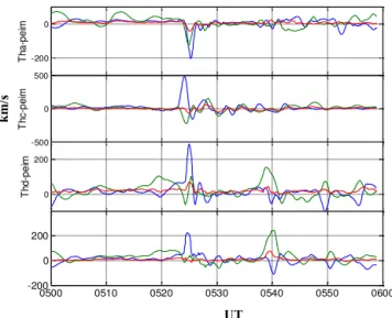
Figure 1.Plasma flow velocity components (blue –Vx, green –Vy,
red –Vz) of TH-A, C, D, and E in GSM coordinates after smoothing
with moving average method.
inferred from the single spacecraft located further west (see Fig. 1; Keiling et al., 2009).
The THEMIS mission measured both the magnetic field and plasma flow velocity fluctuations. As far as the changes in the magnetic field are sharp and the vortex structures are difficult to analyze, in this paper only the data of the plasma flow velocity components will be referred. The event was better catch by the TH-C spacecraft, so in further analysis data only from this one should be used.
The substorm onset caused strong fluctuations of the plasma flow velocity. This sharp change of the field param-eters was detected by all of the spacecrafts (Keiling et al., 2009). The flows of the clustered spacecraft (TH-A, D, and E) show characteristics of a counterclockwise vortex while the spacecraft TH-C detected clockwise rotational field (see Figs. 1, 4).
Figure 1 shows plasma flow velocity components. It is ob-vious that the main vortex is accompanied with the smaller but essential peaks. They are suggested to be the vortex chain or the secondary vortices generated by the first main ones. The idea was that the substorm associated reconnec-tion, which is a strong source of plasma velocity shear – BBF, generates more than one vortex at interaction with the solar wind plasma – a main vortex with the small amplitude satel-lite vortices, which generate the vortex chain in flow.
Based on dataset, analyzed in Keiling et al. (2009), after providing the hodograms of the TH-C data of the plasma flow velocity components, (Fig. 2) several structures (at least, six structures, having rotational sense of motion) are indeed revealed. But this method is not enough to distinguish the nature of these structures. For further analysis vorticity of the plasma flow was estimated also. Vorticity in the mag-netosphere is of importance because it has been associated
-50 0 50 100
-50 0 50 100
-100 -50 0 50
-60 -40 -20 0 20
-200 0 20 40
20 40 60 80
-20 -10 0 10
-20 0 20 40
-500 0 500
-200 0 200
Vy
-100 -50 0 50
-100 0 100
6 5
4
1 2 3
Figure 2.Hodograms of the plasma flow velocities corresponding to the TH-C data.
with field-aligned current (FAC) systems flowing during sub-storms. For this purpose, we seek for the minimal conditions, which give us possibility of determination of the flow vortic-ity by means of spacecraft measurements. In a steady state, vorticity is conserved along the field lines, in which case one might infer much about the ionospheric vortex from magne-tospheric vortex observations. For investigation of the iono-spheric vortices, information about their vorticity is given by the magnetospheric ones. For this purpose, vorticity is esti-mated using the flow velocity components for different satel-lites, linear approximation of which is possible to describe by taking into account the satellite position coordinates and the flow velocity components. Such calculations give a first approximation of the vorticity characteristics.
In a linear approximation for the derivatives of the velocity the following coupled set of equations is given:
Vxi =Vx0+ ∂Vx
∂x dxi0− ∂Vx
∂y dyi0, (4)
Vyi =Vy0+ ∂Vy
∂x dxi0− ∂Vy
∂y dyi0, (5)
wherei=A, B, D is used to represent the closely clustered satellites; index 0 represent the satellite, according to which the calculations are made. Solving the set of equations, we getzcomponent of the flow vorticity
z=
∂Vy
∂x − ∂Vx
∂y . (6)
UT
0 200 400 600 800 1000 1200
-0.2 -0.1 0 0.1 0.2 0.3 0.4 0.5
V
o
rt
ic
it
y
05:00 05:30 06:00
Figure 3.The vorticity of the plasma flow calculated using TH-A, D, E satellites.
300 400 500 600 700 800 900 -200
-150 -100 -50 0 50 100
05:00 05:30 06:00
Vx
Vy
Figure 4.Vector plots of the flow velocity components (projected onto the GSM X–Y plane). Data from TH-C.
sign fast, one can assume that the structures, revealed in the experimental data, represent the vortices of different nature (monopole, dipole).
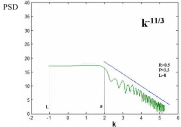
Figure 5 shows the total power spectrum density (PSD) of the magnetic fluctuations (Alexandrova, 2008). The power spectral density of the magnetic field components is calcu-lated using the Morlet wavelet transform. One can see that the high frequency part of the spectrum follows a well de-fined power lawk−11/3.
4 Numerical simulation
The strong turbulence model represents a system of nonlin-ear partial differential equations with inhomogeneous coef-ficients and vector Jacobean type nonlinearity (Aburjania et
PSD
Figure 5.Spectral properties of magnetic fluctuations of a substorm event between 05:00 and 06:00 UT on 19 February 2008.
al., 2002, 2009). The complexity of the numerical analysis of this system is caused by nonlinear terms. The perturbations, obtained by the finite difference schemes for the reduced di-mensionless quantitiesψ, hin some time interval (Aburja-nia et al., 2006) will be self organized into vortex structures, which coincide with analytical ones for such flows. This in-dicates that the solutions obtained at numerical simulation in finite time interval contain also the stationary structures, which together with energetic estimations simplifies an esti-mation of simulation accuracy.
The initial and boundary value problem for time depen-dent dimensionless equation was solved numerically by us-ing an implicit finite difference scheme described in (Abur-jania et al., 2011). The computations were carried out on a 200×200 mesh in thex andy coordinates. The correctness of the computations and the stability of the scheme were con-trolled by solving model problems and also by checking the conservation of the mass of the structure and perturbation en-ergy. The mass and energy were conserved with an accuracy of no worse than 10−2.
Figure 6 represents evolution of initial monopole and ran-dom perturbations of the plasma flow, localized in a circle of radius 0.2 and magnetic field in a Gaussian inhomoge-neous flows, whereV0(y)=Vmexp(−y2/L2y), whereLy is
transversal scale of the flowLy=(2−3)R. Interaction of the
y
ψ h
-5 0 5
-5 0 5
-5 0 5
-5 0 5
y
x x
Figure 6.Evolution of localized randome disturbances of the stream functionψand the magnetic inductionhin timet=3.
are dependent on the characteristics of BBF, its profile, am-plitude and inhomogeneity and as far as the form of the BBF is dependent on solar wind dynamics, generated structures are defined by the solar wind and magnetic field interaction. Numerical analysis shows, that chain generation changes as the characteristics of the flow also magnetic field parame-ters. So, generated magnetic field perturbations depend on the structures generated in the flow and it is clear from Fig. 6, that, the structures will also be generated when the initial magnetic perturbation is zero. The structure is more com-plicated, which is in good agreement with experimental data (Keiling et al., 2009).
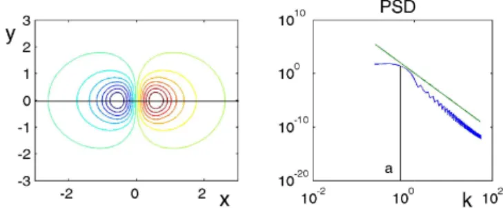
It is also very interesting to estimate a PSD) of analytical stationary dipole solution (Aburjania et al., 2009). The vor-tex structures form energetic spectra and participate in BBF flow energy balance. In this case we simulated a scenario of a magnetic probe moving along thexaxis with a constant ve-locity and a distance of closest approach to the vortex axisx. The Fig. 7 shows the power spectral densities (PSD) of these signals calculated via the Morlet Wavelet Transforms. The power spectra of dipole have a knee around the wave vector
k=1, corresponding to a radiusa=0.83. The dipolar vor-tex spectrum on this case follows power lawk−6.
Note that these spectra are not completely independent of the trajectory of the virtual probe through the vortices. Along some particular trajectories, the magnetic field com-ponents are equal to zero and then the spectrum vanishes. These trajectories are vortex separatrices. Actually, the prob-ability that the satellite crosses the vortex along a separatrix is small and the spectra of Fig. 7 can be considered as quasi-universal. The vortex spectra presented above can partially explain the magnetic spectrum presented in Fig. 5. Dipole vortex model reproduces the spectral knee, it appears to be around k=a−1. The rather steep power laws of the dipole
structures can explain the important steepening of the spec-trum.
5 Conclusions and discussions
In this work, we investigated collective processes in mag-netized plasma, caused by nonlinear regular structures. It is
Figure 7.Dipolar vortex and corresponding PSD, describing the characteristics of this dipole: vortex radius (a), distance between the vortices (l) and power low (P):a=0.83,l=0,P= −6. Black line on the left figure is the vortex separatrix.
Table 1.Characteristics of the vortex structures.
TH-C 1 (70) Structure 2 (70) Structure 3 (70) Structure 4 (65) Structure 5 (80) Structure 6 (50) Structure
Time Scale 210 s 210 s 210 s 195 s 240 s 150 s
Average velocity 148 km s−1 47.4 km s−1 12 km s−1 33 km s−1 36 km s−1 7 km s−1
Size 31 080 km 9870 km 2520 km 6435 km 8640 km 1050 km
during the earthward flow bursts. The tailward-directed flow burst forces vortex chain formation on the two sides of the BBF funnel similar to “von Karman street” (see Fig. 6) with change their sense of rotation. Indeed, numerical 2-D MHD simulations revealed presence of both configurations during the oscillatory BBF braking (see Figs. 6 and 7). Therefore, the results of this analysis are important for understanding of the magnetosphere – ionosphere coupling phenomena.
The substorm on 19 February 2008 developed a sub-storm surge that propagated poleward, westward, and east-ward which is typical for substorms (Akasofu, 1976). Four THEMIS spacecraft monitored in situ the conjugate space vortices. One space vortex engulfed the three clustered spacecraft, which were separated in a triangular-like constel-lation (1–2 RE), allowing an unambiguous identification of a counterclockwise flow. The associated clockwise vortex was tentatively inferred from the single spacecraft located fur-ther west. The experimental data treatment revealed several smaller vortices with the main one, associated with the sub-storm onset. Further analysis has shown that the rotational senses of these smaller space vortices were consistent with the main ones. Their characteristic sizes and time scales are also estimated for all the spacecrafts, but only for TH-C is given in Table 1.
Regarding the mapping of a flow vortex from the mag-netosphere to the ionosphere, Borovsky and Bonnell (2001) showed theoretically that the ionospheric footprint of a pos-itive (downward current) vortex is larger than the mapped footprint of the corresponding magnetospheric vortex be-cause of a spreading of the associated electric potential from high to low altitude. Hence, the larger EIC vortex (600– 800 km) versus the smaller mapped footprint (180 km) could be explained by this spreading and/or because the THEMIS spacecraft did not enclose the entire space vortex (Keiling et al., 2009). Assuming conservation of angular speed, the flow speed of 300–900 km s−1corresponds to 4–12 km s−1in the
ionosphere. However, this assumption is most likely not valid because of ionospheric drag, and thus the mapped speeds should only be considered as an upper limit. Additional anal-ysis of the ionospheric experimental satellite and ground-based data is necessary for magnetosphere-ionosphere cou-pling processes in a separate study.
Acknowledgements. Shota Rustaveli National Science Founda-tion’s Grant no 31/14.
Edited by: M. Förster
Reviewed by: two anonymous referees
References
Aburjania, G., Khantadze, A., and Kharshiladze, O.: Nonlinear planetary electromagnetic vortex structures in F region of the ionosphere, Plasma Phys. Rep., 28, 633–638, 2002.
Aburjania, G. D.: Self-Organization of the Nonlinear Vortex Struc-tures and the Vortical Turbulence in the Dispersive Media: Kom-Kniga, Editorial URSS, Moscow, Russia, 2006.
Aburjania, G. D., Chargazia, Kh. Z., Zelenyi, L. M., and Zimbardo, G.: Model of strong stationary vortex turbulence in space plas-mas, Nonlin. Processes Geophys., 16, 11–22, doi:10.5194/npg-16-11-2009, 2009.
Akasofu, S.-I.: Physics of Magnetospheric Substorms, D. Reidel Publ. Co., Dordrecht, the Netherlands, 1976.
Alexandrova, O.: Solar wind vs magnetosheath turbulence and Alfvén vortices, Nonlin. Processes Geophys., 15, 95–108, doi:10.5194/npg-15-95-2008, 2008.
Angelopoulos, V.: The THEMIS Mission, Space Sci. Rev., 141, 5– 34, doi:10.1007/s11214-008-9336-1, 2008.
Birn, J., Raeder, J., Wang, Y. L., Wolf, R. A., and Hesse, M.: On the propagation of bubbles in the geomagnetic tail, Ann. Geophys., 22, 1773–1786, doi:10.5194/angeo-22-1773-2004, 2004. Biskamp, D., Schwarz, E., Zeiler, A., Celani, A., and Drake, J. F.:
Electron magnetohydrodynamic turbulence, Phys. Plasmas., 6, 751–758, 1999.
Borovsky, J. and Bonnell, J.: The DC electrical coupling of flow vortices and flow channels in the magnetosphere to the resistive ionosphere, J. Geophys. Res., 106, 28967–28994, 2001. Chmyrev, V. M., Marchenko, V. A., Pokhotelov, O. A., Stenflo, L.,
Streltsov, A. V., and Steen, A.: Vortex structures in the iono-sphere and the magnetoiono-sphere of the Earth, Planet. Space Sci., 39, 1025–1037, 1991.
Cho, J. and Lazarian, A.: The anisotropy of magnetohydrodynamic turbulence, Astrophys. J., 615, L41–L44, 2004.
Diamond, P. H. and Carreras, B. A.: On mixing length theory and saturated turbulence, Comm. Plasma Phys. Contr. Fus., 10, 271– 278, 1987.
Galeev, A. A. and Sagdeev, R. Z.: Nonlinear Theory of plasma, in: Reviews of Plasma Physics, edited by: Leontovich, M. A., Con-sultant Bureau, New York, USA, Vol. 7, 1976.
tur-bulence, Phys. Plasmas, 12, 092310, doi:10.1063/1.2052507, 2005.
Gekelman, W.: Review of laboratory experiments on Alfven waves and their relationship to space observations, J. Geophys. Res., 104, 14417–14435, 1999.
Goldreich, P. and Sridhar S.: Toward a theory of interstellar turbu-lence, II. Strong Alfvenic turbuturbu-lence, Astrophys. J., 438, 763– 775, 1995.
Horton, W.: Nonlinear Drift Waves and Transport in Magnetized Plasma, Review, Institute for Fusion Studies the University of Texas at Austin, IFSR, Austin, Texas, USA, 1990.
Howes, G. G., Cowley, S. C., Dorland, W., Hammettm G. W., Quataertm E., and Schekochihinm A. A.: A model of tur-bulence in magnetized plasmas: Implications for the dissipa-tion range in the solar wind, J. Geophys. Res., 113, 05103, doi:10.1029/2007JA012665, 2008.
Iroshnikov, R. S.: The turbulence of a conducting fluid in a strong magnetic field, Astr. Zh., 40, 742–750, 1963.
Keiling, A., Angelopoulos, V., Runov, A., Weygand, J., Apatenkov, S. V., Mende, S., McFadden, J., Larson, D., Amm, O., Glass-meier, K.-H., and Auster, H. U.: Substorm current wedge driven by plasma flow vortices: THEMIS Observations, J. Geophys. Res., 114, A00C22, doi:10.1029/2009JA014114, 2009. Keika, K., Nakamura, R., Volwerk, M., Angelopoulos, V.,
Baumjo-hann, W., Retinò, A., Fujimoto, M., Bonnell, J. W., Singer, H. J., Auster, H. U., McFadden, J. P., Larson, D., and Mann, I.: Ob-servations of plasma vortices in the vicinity of flow-braking: a case study, Ann. Geophys., 27, 3009–3017, doi:10.5194/angeo-27-3009-2009, 2009.
Kingsep, A. S.: Introduction to the Nonlinear Plasma Physics, in: Reviews of Plasma Physics, edited by: Kadomtsev, B. B., Con-sultant Bureau, New York, USA, Vol. 16, 1990.
Kolmogorov, A. N.: Local structure of turbulence in the noncom-presible viscous fluid at very high Reynolds number, Dokl. Akad. Nauk. SSSR, 30, 299–303, 1941.
Kraichnan, R. H.: Inertial range spectrum hydromagnetic turbu-lence, Physics of Fluids, 8, 1385–1387, 1965.
McFadden, J., Carlson, C. W., Larson, D., Ludlam, M., Abiad, R., Elliott, B., Turin, P., Marckwordt, M., and Angelopoulos, V.: Space Sci. Rev., 141, 277–302, 2008.
Matthaeus, W. H., Oughton, S., Pontius, D. H., and Zhou, Y.: Evo-lution of energy-containing turbulent eddies in the solar wind, J. Geophys. Res., 99, 19267–19287, 1994.
Müller, W.-C., Biskamp, D., and Grappin, R.: Statistical anisotropy of magnetohydrodynamic turbulence, Phys. Rev. E., 67, 066302, doi:10.1103/PhysRevE.67.066302, 2003.
Narita, Y., Glassmeier, K.-H., Fränz, M., Nariyuki, Y., and Hada, T.: Observations of linear and nonlinear processes in the fore-shock wave evolution, Nonlin. Processes Geophys., 14, 361–371, doi:10.5194/npg-14-361-2007, 2007.
Nezlin, M. V. and Snezhkin, E. N.: Rossby Vortices, Spiral Struc-tures, Solitons, Springer-Verlag, Heidelberg, Germany, 1993. Panov, E. V., Nakamura, R., Baumjohann, W., Angelopoulos, V.,
Petrukovich, A. A., Retinò, A., Volwerk, M., Takada, T., Glass-meier, K.-H., McFadden, J. P., and Larson, D.: Multiple over-shoot and rebound of a bursty bulk flow, J. Geophys. Res., 37, L08103, doi:10.1029/2009gl041971, 2010.
Richardson, L. F.: Wheather Prediction of “Numerical Method”, Cambridge University Press, Cambridge, UK, 1922.
Sahraoui, F., Belmont, G., Pinçon, J. L., Rezeau, L., Balogh, A., Robert, P., and Cornilleau-Wehrlin, N.: Magnetic turbulent spec-tra in the magnetosheath: new insights, Ann. Geophys., 22, 2283–2288, doi:10.5194/angeo-22-2283-2004, 2004.
Sahraoui, F., Belmont, G., Rezeau, L., and Cornilleau-Wehrlin, N.: Anisotropic turbulent spectra in the terrestrial magnetosheath as seen by the Cluster spacecraft, Phys. Rev. Lett., 96, 075002, doi:10.1103/PhysRevLett.96.075002, 2006.
Snekvik, K., Haaland, S., Østgaard, N., Hasegawa, H., Nakamura, R., Takada, T., Juusola, L., Amm, O., Pitout, F., Rème, H., Klecker, B., and Lucek, E. A.: Cluster observations of a field aligned current at the dawn flank of a bursty bulk flow, Ann. Geo-phys., 25, 1405–1415, doi:10.5194/angeo-25-1405-2007, 2007. Zimbardo, G.: Magnetic turbulence in space plasmas in and around