www.ann-geophys.net/25/847/2007/ © European Geosciences Union 2007
Annales
Geophysicae
Variability of Jovian ion winds: an upper limit for enhanced Joule
heating
M. B. Lystrup1,2, S. Miller1,2, T. Stallard1, C. G. A. Smith1, and A. Aylward1
1Department of Physics & Astronomy, University College London, Gower Street, London WC1E 6BT, UK
2Visiting Astronomer at the Infrared Telescope Facility, which is operated by the University of Hawaii under Cooperative Agreement no. NCC 5-538 with the National Aeronautics and Space Administration, Science Mission Directorate, Planetary Astronomy Program
Received: 29 September 2006 – Revised: 19 March 2007 – Accepted: 27 March 2007 – Published: 8 May 2007
Abstract. It has been proposed that short-timescale fluc-tuations about the mean electric field can significantly in-crease the upper atmospheric energy inputs at Jupiter, which may help to explain the high observed thermospheric tem-peratures. We present data from the first attempt to detect such variations in the Jovian ionosphere. Line-of-sight iono-spheric velocity profiles in the Southern Jovian auroral/polar region are shown, derived from the Doppler shifting of H+3 infrared emission spectra. These data were recently obtained from the high-resolution CSHELL spectrometer at the NASA Infrared Telescope Facility. We find that there is no vari-ability within this data set on timescales of the order of one minute and spatial scales of 640 km, putting upper limits on the timescales of fluctuations that would be needed to en-hance Joule heating.
Keywords. Magnetospheric physics (Auroral phenomena) – Ionosphere (Ionosphere-atmosphere interactions; Planetary ionospheres)
1 Introduction
The origin of the remarkably high thermospheric tempera-tures of Jupiter (and indeed all the gas giant planets), con-firmed by measurements from the Voyager (Atreya, 1986) and Galileo spacecraft (Seiff et al., 1997) and from ground-based observations (Stallard et al., 2002) to be∼900 K, re-mains unexplained. Solar heating cannot, by itself, account for these temperatures (Strobel and Smith, 1973) and vari-ous additional energy sources have been suggested. From as early as 1983, energy from particles precipitated into the up-per atmosphere in auroral regions has been considered (Waite et al., 1983; Grodent and G´erard, 2001). Normal Joule heat-ing (calculated usheat-ing the average ionospheric electric field) Correspondence to: M. B. Lystrup
(Cowley et al., 2005) and ion drag (Miller et al., 2000) have been suggested as possible heat sources, as well as gravity waves (Young et al., 1997) and acoustic waves (Schubert et al., 2003). However, none of these additional energy inputs have been demonstrated unambiguously to explain the en-ergy gap (Matcheva and Strobel, 1999; Hickey et al., 2000).
Joule heating in the upper atmosphere is the result of rel-ative motion between neutrals and ions – the thermalization of kinetic energy (Cowley et al., 2004). Electric fields are generated by plasma flows in the magnetosphere and map along magnetic field lines into the upper atmosphere, result-ing in bulk ion flows. The jovian equatorial plasma sheet, constantly fed by material from Io, receives rotational energy from Jupiter that keeps the plasma sheet in corotation with the planet. At around 20 Jovian radii from the planet, corota-tion begins to break down (Hill, 1979), generating a current system that closes through the ionosphere. This mechanism implies an equatorward field across the auroral oval, where a near-perpendicular planetary magnetic field exists. The re-sult is a westward (Hall) ion drift – an ion wind – around the oval, with a magnitude given by vion=Eeq/BJ, where Eeq is the equatorward electric field and BJ is the Jovian
magnetic field at the auroral oval. These ion winds were first detected in the Jovian aurora by Rego et al. (1999) and subse-quent observations have been used to probe the dynamics of and energy balance in the Jovian upper atmosphere (Stallard et al., 2001). Typically,vionis of the order of 1 kms−1; with
BJ≈10−3 Tesla, Eeq must therefore have a value around
1 Vm−1.
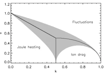
Fig. 1. The standard deviation of the fluctuations,s, is plotted ver-suskshowing the the relative importance of heating mechanisms. The unshaded region indicates where a heating source is dominant by greater than 50%. Figure from Smith et al. (2005).
magnetospheric inputs to Jupiter’s ionosphere over several Jovian rotations could result in considerable excess heating of the upper atmosphere. All of these studies, however, deal with variations whose timescales are on the order of, or con-siderably greater than, the time taken for the thermosphere (the main component of the upper atmosphere) to respond to changes in the velocity of the ions: for Jupiter, modelling by Millward et al. (2005) indicates that this thermospheric response time should be on the order of 1500 s.
For the Earth, Codrescu et al. (1995) suggested that cal-culations considering only the average electric field, ignor-ing fluctuations on timescales shorter than the thermospheric response time, underestimate Joule heating for the high-latitude regions. The first direct evidence supporting this was found by northern auroral measurements of Earth’s thermo-sphere by Aruliah et al. (2005). They found that the vari-ations on timescales of one minute in the electric field do indeed contribute significantly to Joule heating. Smith et al. (2005) argued that, similar to the case in Earth’s ionosphere, persistent short-timescale fluctuations about the mean elec-tric field could significantly increase the average Joule heat-ing in the upper atmosphere of Jupiter. To explain this, they expressed the Joule heating and the ion drag (the kinetic en-ergy) in the rest frame of the neutrals as, respectively:
QJ =(1−k)26PE2 (1)
QI D =k(1−k)26PE2 (2)
where 6P is the Pedersen conductivity, E is the electric
field, andkis defined as k=vn/vi, wherevn is the neutral
wind velocity andviis the westward ion drift velocity. They
then considered the full, fluctuating electric field as a sum of
the mean electric fieldEand the random fluctuationsf (t ), which have some statistical distribution with a mean of zero and variancef2=s2:
Ef(t )=E(1+f (t )) (3)
The neutrals cannot respond to changes in the ion wind on short timescales and are therefore insensitive to rapid varia-tions in the electric field. Thus, Smith et al. (2005) showed that the time-averaged Joule heating becomes:
QJf = [(1−k)2+s2]6PE2 (4)
The magnitude of the Joule heating component from the fluc-tuating electric field,s26PE2, is independent ofk and de-pends only on the variance. However, the relative importance of this component from fluctuations depends also onk. The value ofkis unknown, but some models have predicted it to be as high as 0.7 for the peak of the Jovian ion density (Mill-ward et al., 2005). Figure 1 shows the relative importance of Joule heating, Joule heating from electric field fluctuations, and ion drag (which is unaffected by electric field fluctua-tions) for a range ofkand standard deviation (s) values. Ifs
is 1.0, which means the fluctuations in the field are of mag-nitude of the mean of the field, the contributed Joule heating is significant no matter the value ofk. The fluctuations in Earth’s electric field observed by Aruliah et al. (2005) have
s of 1.0. (Note thatk is not generally considered a useful parameter with respect to Earth.) Forkvalues predicted by models of Jupiter (Cowley and Bunce, 2001), around 0.5, the standard deviation of the fluctuations needed to enhance Joule heating significantly must be around 0.6.
These fluctuations do not have a preferential time scale, as long as the time scale is short enough that the neutrals do not have enough time to respond to the change in electric field – on order of 1500 s (Millward et al., 2005); the ions respond immediately. Aruliah et al. (2005) found fluctuations signif-icant on the order of one minute, but insignifsignif-icant for Joule heating on the order of 15 min. It is also unknown if a pre-ferred size scale exists for the fluctuations.
Evidence for turbulence in the Jovian middle magneto-sphere has been seen in an analysis of Galileo data and it has been suggested that this turbulence could affect resistiv-ity along magnetic field lines and alter the Hill (1979) mech-anism that couples the Jovian atmosphere with the magneto-sphere (Saur et al., 2002). This turbulence might also drive electric field fluctuations that would lead to an enhanced Joule heating effect. Given a constant value ofBJ,
fluctu-ations in the ionospheric electric field,Eeq, would result in
from the planet, at which distance they estimated Alfv´en travel times in the magnetosphere to be 375 s per Jovian ra-dius (1RJ=71 492 km). This would make the Alfv´en travel
time from 20RJ to the planet itself be 7500 s.
2 Observations
On 5 May 2006 the CSHELL echelle spectrometer (Greene et al., 1993) at the NASA Infrared Telescope Facility (IRTF) on Mauna Kea, Hawaii was used to collect these data. We chose to observe the Q(1,0−)emission line in theν2 funda-mental vibrational band of the H+3 molecular ion. This emis-sion line has been used successfully to probe Jupiter’s upper atmosphere in many other studies (Rego et al., 1999; Stallard et al., 2001, 2004; Melin et al., 2005). Ground-based infrared observations of the Q(1,0−)line and other bright emission features of H+3 are possible because they lie within Earth’s atmospheric L’ window and fall within a wavelength region in which Jupiter’s IR continuum spectrum is suppressed by stratospheric methane absorption.
CSHELL’s circular variable filter was set to pick out 3.953µm, the wavelength of the Q(1,0−)line. The
instru-ment was rotated at an angle of 71.8◦such that the slit was positioned to cut east-west across the entire auroral oval, per-pendicular to Jupiter’s rotational axis which had a position angle of 18.2◦on 5 May (see Fig. 2). We attempted to keep the slit in the same position throughout the night, but some drift resulted from the limitations of the guiding system’s ability to track an extended object. Images of Jupiter at K-band in CSHELL’s direct imaging mode were made and used to align the slit along the polar limb and calculate telescope offsets. Images at 3.953µm were used at the data analysis stage to find the exact slit position on the planet.
Apparent wavelength shifts can be introduced due to un-even illumination across a slit, and the surface brightness of the Jovian aurora varies on a variety of spatial scales. In pre-vious studies, CSHELL images taken at 3.953µm have been used to correct for the minor discrepancies due to this effect (Stallard et al., 2001). In recent years, however, the quality of these images has degraded such that corrections for spa-tial effects are difficult to apply. In order to minimize this effect, the narrowest slit width available on CSHELL, 0.5”, was chosen giving spatial resolution of 0.2” per pixel. At 3.953µm, this slit gives a resolving power ofλ/1λ∼40 000.
We made spectral observations of Jupiter in an ABBA nod-to-sky pattern (where A is an object exposure and B is a sky exposure), but because we were interested in minute-to-minute variations, we also made observations in an AB/A/AB pattern to minimize the time between sky expo-sures. For Jovian spectra we used an integration time of 50 s, as that time has previously yielded good signal-to-noise. Af-ter 10 JupiAf-ter exposures, we took an image at K-band and at 3.953µm. This observing strategy was implemented on both the Northern and the Southern aurorae; the Northern aurora
Fig. 2. A schematic diagram of the slit position across the southern
auroral region of Jupiter for a CML of 334. The solid curve is the 30RJoval and the triangles are the Io footprint, both from the VIP4
model of Connerney et al. (1998).
was relatively weak, however, so only the higher-intensity Southern data are presented for this analysis. The relative weakness of the northern auroral emission is an interesting observation, which we have noted in other (unpublished) data, and which we shall address in a future publication.
3 Data reduction and analysis
Spectra were reduced using standard infrared techniques of sky-subtracting, flat-fielding, removing bad pixels, and wavelength calibration. For each spectral row across the planet, the spectrum was fitted with a Gaussian fitting pro-cedure. Peak intensities, line positions, and line widths for the spectral rows were recorded.
Velocity profiles were calculated from the Doppler-shifting of the Q(1,0−)line. In addition to the actual ve-locity of the ion winds, this measured veve-locity includes com-ponents due to the rotation of the planet, the nonlinearity of the array’s wavelength scale, and an arbitrary shift from zero. The details of correcting for these factors can be found in Stallard et al. (2001). The zero-position of the velocity was set where the emission from the H+3 has zero velocity – on the dusk side of the planet between the auroral oval and the limb. H+3 emission does exist in this region, but it is not as-sociated with the electrojet or other ion wind systems. The velocity profiles presented here have, as explained above, not been subject to correction for uneven illumination across the slit. This may affect the actual velocity measurements, al-though it is minimized in the Southern Hemisphere where the viewing angle of the oval from Earth tends to average out these effects. After these corrections we are left with the line-of-sight, non-spatially-corrected velocity profiles (Stal-lard et al., 2001):
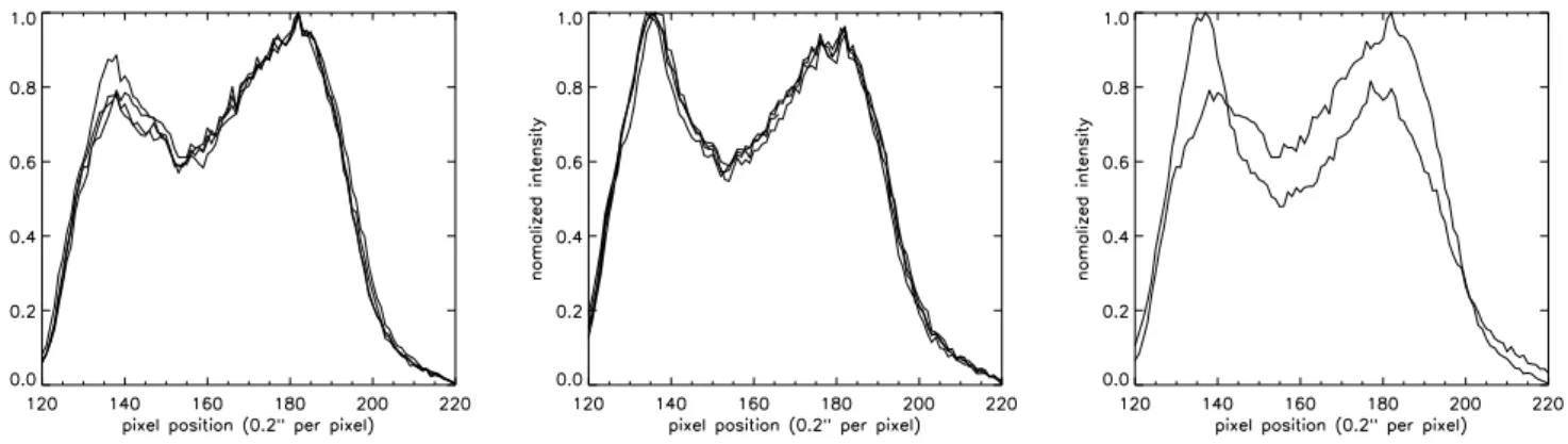
Fig. 3. The first and second plot shows the intensity profiles of spectra in Group 1 and Group 2, respectively. The last plot shows two
consecutive spectra, taken only 55 s apart, that have clearly different intensity morphologies, and were thus taken at different latitudes due to an inability to keep the slit stationary on the planet.
Table 1. Spectra considered in this study.
Group 1 Group 2
File No. UT CML Airmass File No. UT CML Airmass 151 10:36:04.05 330.244 1.221 159 10:43:26.09 334.701 1.225 156 10:40:42.00 333.047 1.223 160 10:44:21.06 335.255 1.226 157 10:41:37.00 333.601 1.224 161 10:45:16.06 335.810 1.227 158 10:42:31.09 334.146 1.225 162 10:46:11.06 336.365 1.227
of spectra with the same intensity profiles were assumed to have been taken to be at the same latitude. These conditions were satisfied for two sets of four spectra, as listed in Ta-ble 1. In both groups the intensity profiles closely match, as seen in Fig. 3. Consecutive spectra did not always fit this condition; the same figure shows another pair of consecutive spectra with very different intensity profiles, clearly affected by drift in the telescope pointing, which were not analyzed further.
For each group, the mean of the four velocity profiles and each profile’s difference from that mean were calculated. For comparison, model profiles were created assuming a normal distribution of fluctuations with different variances and with mean equal to the mean of the observed velocity profiles. The model profiles were smoothed to 3 pixels to simulate the 0.6” seeing conditions that existed during our observations. These simple model profiles show what we might expect our observed velocity profiles to look like if fluctuations exist.
4 Results and discussion
For both groups of spectra showing near-identical intensity profiles, the mean of the four velocity profiles and each pro-file’s difference from that mean were calculated. These are shown for Group 1 in Fig. 4. For comparison, model profiles
were created assuming a normal distribution of fluctuations with different variances and with mean equal to the mean of the observed velocity profiles. The model profiles were smoothed to 3 pixels to simulate the 0.6” seeing conditions that existed during our observations. These simple model profiles reveal what we might expect our observed velocity profiles to look like if fluctuations do exist.
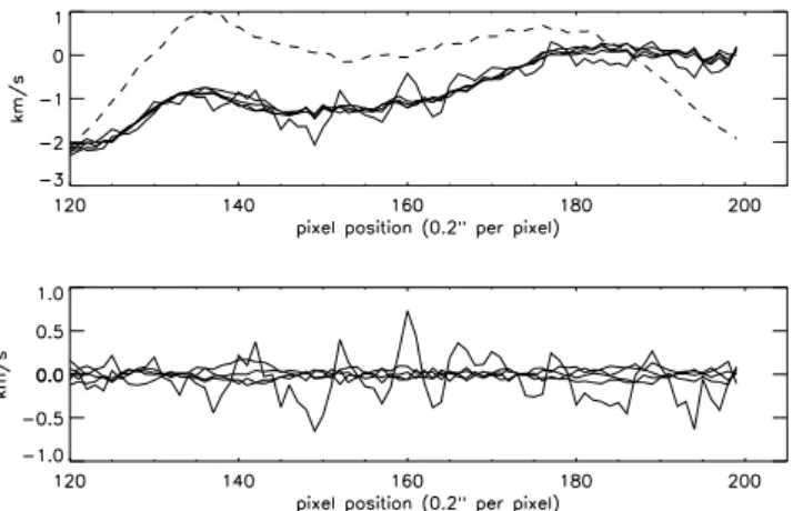
Fig. 4. The four spectra from Group 1 are shown (top) with
varia-tions from the group average (bottom). The bold lines are the model profile and fluctuations from the Group 1 average assumings=1.0, smoothed to three pixels to estimate seeing effects. The large nega-tive velocities seen between pixels∼122 and 132 are due to uneven
illumination across the slit as it crosses the dawn limb of the planet. The dashed curve is the average intensity profile for this group of spectra, scaled to the velocity.
In bold in Fig. 4 is a model profile with a mean equal to the Group 1 mean and standard deviations=1. For this model the velocity structure is dominated by 1 kms−1 varia-tions. But the observed variations are of less than 200 ms−1, which is at the resolution limit of CSHELL. Figure 5 shows the corresponding data for Group 2, this time plotted with the model profile usings=0.5, the lowest estimate that signifi-cantly contributes to heating (Smith et al., 2005). The model fluctuations also remain significantly larger than those we ob-served. We therefore conclude that we are not able to observe fluctuations that would contribute significantly to Joule heat-ing within our current dataset.
The longest sequence of spectra that we feel confident in using for this study span approximately 250 s. This is a significant fraction of the thermospheric response time of around 1500 s, and it is thus unlikely that fluctuations on a time scale much longer than this will contribute signifi-cantly to the enhanced Joule heating considered by Smith et al. (2005) since some thermospheric damping of the effect will occur. Fluctuations occurring over a shorter time scale than we tested might also occur and, since the thermosphere could not respond to these, would be important. What this study has provided is, therefore, a significant upper limit to the timescale for variations in the atmospheric current that can contribute to the “missing” heating in the upper atmo-sphere via the Smith et al. (2005) mechanism of enhanced Joule heating.
One explanation as to why we did not observe fluctuations on the timescale of one minute or so, even though Saur et al. (2002) did see them in the magnetosphere, could be that the
Fig. 5. The four spectra from Group 2 are shown (top) with
varia-tions from the group average (bottom). The bold lines are the model profile and fluctuations from the Group 2 average assumings=0.5, smoothed to three pixels to estimate seeing effects. As in Fig. 4, the large negative velocities seen between pixels∼122 and 132 are due
to uneven illumination across the slit as it crosses the dawn limb of the planet. Note that the velocity structure is the same as in Fig. 4. The dashed curve is the average intensity profile for this group of spectra, scaled to the velocity.
Alfv´en travel time, around 7500 s, is sufficiently long that these fluctuations are damped out en route from the middle magnetosphere to the upper atmosphere. For our observa-tional configuration, CSHELL’s effective spatial resolution is about 640 km by 640 km and it is also possible that the fluc-tuations that contribute significantly to Joule heating are on a smaller spatial scale, such that we miss them in our obser-vations; successful observations of electric field fluctuations at Earth used spatial scales far finer than ours (Aruliah et al., 2005).
5 Conclusions
Our results are from the first attempt to probe the idea of Joule heating from short-timescale electric field fluctuations in the Jovian upper atmosphere using observational tech-niques. We have shown that on the timescale of one minute there is no variability in the Jovian auroral ion velocities, av-eraged over spatial scales of 640 km. This provides an upper limit on the timescale of fluctuations that would contribute to enhanced Joule heating. Future observations, using shorter integration times, will be able to examine shorter timescale variations. They will perhaps also need to coincide with those occasions when clear views of the polar cap regions are available.
Acknowledgements. It is a pleasure to acknowledge the IRTF staff
for their expert assistance during our observations. T. Stallard was supported by a UK Particle Physics and Astronomy Research Coun-cil (PPARC) postdoctoral fellowship. C. G. A. Smith was funded by a Case studentship from Sun Microsystems and PPARC. The team reporting here is part of the EuroPlaNet European planetary science network, which is supported by the European Union Framework 6 programme. We express our thanks to the anonymous referee who contributed helpful comments that improved this paper.
Topical Editor M. Pinnock thanks two referees for their help in evaluating this paper.
References
Aruliah, A. L., Griffin, E. M., Aylward, A. D., Ford, E. A. K., Kosch, M. J., Davis, C. J., Howells, V. S. C., Pryse, S. E., Mid-dleton, H. R., and Jussila, J.: First direct evidence of meso-scale variability on ion-neutral dynamics using co-located tristatic FPIs and EISCAT radar in Northern Scandinavia, Ann. Geo-phys., 23, 147–162, 2005,
http://www.ann-geophys.net/23/147/2005/.
Atreya, S. K.: Atmospheres and Ionospheres of the Outer Planets and their Satellites, Atmospheres and Ionospheres of the Outer Planets and their Satellites, XIII, 224 pp. 90 figs. (partly in color), Springer-Verlag Berlin Heidelberg New York, also: Phys. Chem. Space, volume 15, 1986.
Codrescu, M. V., Fuller-Rowell, T. J., and Foster, J. C.: On the importance of E-field variability for Joule heating in the high-latitude thermosphere, Geophys. Res. Lett., 22, 2393–2396, doi:10.1029/95GL01909, 1995.
Connerney, J. E. P., Acu˜na, M. H., Ness, N. F., and Satoh, T.: New models of Jupiter’s magnetic field constrained by the Io flux tube footprint, J. Geophys Res., 103, 11 929–11 940, doi:10.1029/97JA03726, 1998.
Cowley, S. W. H. and Bunce, E. J.: Origin of the main auroral oval in Jupiter’s coupled magnetosphere-ionosphere system, Planet. Space Sci., 49, 1067–1088, 2001.
Cowley, S. W. H., Bunce, E. J., and O’Rourke, J. M.: A simple quantitative model of plasma flows and currents in Saturn’s po-lar ionosphere, J. Geophys. Res. (Space Physics), 109, 5212, doi:10.1029/2003JA010375, 2004.
Cowley, S. W. H., Alexeev, I. I., Belenkaya, E. S., Bunce, E. J., Cottis, C. E., Kalegaev, V. V., Nichols, J. D., Prang´e,
R., and Wilson, F. J.: A simple axisymmetric model of magnetosphere-ionosphere coupling currents in Jupiter’s polar ionosphere, J. Geophys. Res. (Space Physics), 110, 11 209, doi:10.1029/2005JA011237, 2005.
Dungey, J. W.: Interplanetary Magnetic Field and the Auroral Zones, Phys. Rev. Lett., 6, 47–48, doi:10.1103/PhysRevLett.6.47, 1961.
Greene, T. P., Tokunaga, A. T., Toomey, D. W., and Carr, J. B.: CSHELL: a high spectral resolution 1–5µm cryogenic echelle spectrograph for the IRTF, in: Proc. SPIE Vol. 1946, p. 313–324, Infrared Detectors and Instrumentation, edited by: Fowler, A. M., pp. 313–324, 1993.
Grodent, D. and G´erard, J.-C.: A self-consistent model of the Jovian auroral thermal structure, J. Geophys Res., 106, 12 933–12 952, doi:10.1029/2000JA900129, 2001.
Grodent, D., Clarke, J. T., Waite, J. H., Cowley, S. W. H., G´erard, J.-C., and Kim, J.: Jupiter’s polar auroral emissions, J. Geophys. Res. (Space Physics), 108, 6–1, doi:10.1029/2003JA010017, 2003.
Hickey, M. P., Walterscheid, R. L., and Schubert, G.: Gravity Wave Heating and Cooling in Jupiter’s Thermosphere, Icarus, 148, 266–281, doi:10.1006/icar.2000.6472, 2000.
Hill, T. W.: Inertial limit on corotation, J. Geophys Res., 84, 6554– 6558, 1979.
Matcheva, K. I. and Strobel, D. F.: Heating of Jupiter’s Ther-mosphere by Dissipation of Gravity Waves Due to Molec-ular Viscosity and Heat Conduction, Icarus, 140, 328–340, doi:10.1006/icar.1999.6151, 1999.
Melin, H., Miller, S., Stallard, T., and Grodent, D.: Non-LTE effects on H+3 emission in the jovian upper atmosphere, Icarus, 178, 97– 103, doi:10.1016/j.icarus.2005.04.016, 2005.
Melin, H., Miller, S., Stallard, T., Smith, C., and Grodent, D.: Estimated energy balance in the jovian upper atmo-sphere during an auroral heating event, Icarus, 181, 256–265, doi:10.1016/j.icarus.2005.11.004, 2006.
Miller, S., Achilleos, N., Ballester, G. E., Lam, H. A., Ten-nyson, J., Geballe, T. R., and Trafton, L. M.: Mid-to-Low Latitude H+3 Emission from Jupiter, Icarus, 130, 57–67, doi:10.1006/icar.1997.5813, 1997.
Miller, S., Achilleos, N., Ballester, G. E., Geballe, T. R., Joseph, R. D., Prang´e, R., Rego, D., Stallard, T., Tennyson, J., Trafton, L. M., and Waite, Jr., J. H.: The role of H+3 in planetary at-mospheres, in: Astronomy, physics and chemistry of H+3, pp. 2485–2502, 2000.
Millward, G., Miller, S., Stallard, T., Achilleos, N., and Aylward, A. D.: On the dynamics of the jovian ionosphere and thermo-sphere., Icarus, 173, 200–211, doi:10.1016/j.icarus.2004.07.027, 2005.
Rego, D., Achilleos, N., Stallard, T., Miller, S., Prang´e, R., Dougherty, M., and Joseph, R. D.: Supersonic winds in Jupiter’s aurorae, Nature, 399, 121, doi:10.1038/20121, 1999.
Saur, J., Politano, H., Pouquet, A., and Matthaeus, W. H.: Ev-idence for weak MHD turbulence in the middle magneto-sphere of Jupiter, Astronomy & Astrophysics, 386, 699–708, doi:10.1051/0004-6361:20020305, 2002.
Seiff, A., Kirk, D. B., Knight, T. C. D., Young, L. A., Milos, F. S., Venkatapathy, E., Mihalov, J. D., Blanchard, R. C., Young, R. E., and Schubert, G.: Thermal structure of Jupiter’s upper atmo-sphere derived from the Galileo probe, Science, 276, 102–104, 1997.
Smith, C. G., Aylward, A. D., and Miller, S.: Magnetospheric En-ergy Inputs Into the Thermospheres of Jupiter and Saturn, AGU Spring Meeting Abstracts, pp. A1+, 2005.
Southwood, D. J. and Kivelson, M. G.: A new perspective concern-ing the influence of the solar wind on the Jovian magnetosphere, J. Geophys Res., 106, 6123–6130, doi:10.1029/2000JA000236, 2001.
Stallard, T., Miller, S., Millward, G., and Joseph, R. D.: On the Dynamics of the Jovian Ionosphere and Thermosphere. I. The Measurement of Ion Winds, Icarus, 154, 475–491, doi:10.1006/icar.2001.6681, 2001.
Stallard, T., Miller, S., Millward, G., and Joseph, R. D.: On the Dynamics of the Jovian Ionosphere and Thermosphere. II. The Measurement of H+3 Vibrational Temperature, Col-umn Density, and Total Emission, Icarus, 156, 498–514, doi:10.1006/icar.2001.6793, 2002.
Stallard, T. S., Miller, S., Trafton, L. M., Geballe, T. R., and Joseph, R. D.: Ion winds in Saturn’s southern auroral/polar region, Icarus, 167, 204–211, doi:10.1016/S0019-1035(03)00285-9, 2004.
Strobel, D. F. and Smith, G. R.: On the Temperature of the Jovian Thermosphere., J. Atmos. Sci., 30, 718–725, 1973.
Waite, J. H., Cravens, T. E., Kozyra, J., Nagy, A. F., Atreya, S. K., and Chen, R. H.: Electron precipitation and related aeronomy of the Jovian thermosphere and ionosphere, J. Geophys Res., 88, 6143–6163, 1983.