Substance Abusers and Non-Clinical Individuals in
Intertemporal Choice
Jiuqing Cheng.*, Claudia Gonza´lez-Vallejo.
Department of Psychology, Ohio University, Athens, Ohio, United States of America
Abstract
The single parameter hyperbolic model has been frequently used to describe value discounting as a function of time and to differentiate substance abusers and non-clinical participants with the model’s parameterk. However,ksays little about the mechanisms underlying the observed differences. The present study evaluates several alternative models with the purpose of identifying whether group differences stem from differences in subjective valuation, and/or time perceptions. Using three two-parameter models, plus secondary data analyses of 14 studies with 471 indifference point curves, results demonstrated that adding a valuation, or a time perception function led to better model fits. However, the gain in fit due to the flexibility granted by a second parameter did not always lead to a better understanding of the data patterns and corresponding psychological processes. Thek parameter consistently indexed group and context (magnitude) differences; it is thus a mixed measure of person and task level effects. This was similar for a parameter meant to index payoff devaluation. A time perception parameter, on the other hand, fluctuated with contexts in a non-predicted fashion and the interpretation of its values was inconsistent with prior findings that supported enlarged perceived delays for substance abusers compared to controls. Overall, the results provide mixed support for hyperbolic models of intertemporal choice in terms of the psychological meaning afforded by their parameters.
Citation:Cheng J, Gonza´lez-Vallejo C (2014) Hyperbolic Discounting: Value and Time Processes of Substance Abusers and Non-Clinical Individuals in Intertemporal Choice. PLoS ONE 9(11): e111378. doi:10.1371/journal.pone.0111378
Editor:Pablo Bran˜as-Garza, Middlesex University London, United Kingdom
ReceivedJune 13, 2013;AcceptedOctober 1, 2014;PublishedNovember 12, 2014
Copyright:ß2014 Cheng, Gonza´lez-Vallejo. This is an open-access article distributed under the terms of the Creative Commons Attribution License, which permits unrestricted use, distribution, and reproduction in any medium, provided the original author and source are credited.
Funding:The authors have no support or funding to report.
Competing Interests:The authors have declared that no competing interests exist.
* Email: [email protected]
.These authors contributed equally to this work.
Introduction
Psychological research on behavioral control has widely used the intertemporal choice paradigm with results generally demon-strating a preference for immediate, smaller rewards over delayed, larger ones by animals and humans. This result is termed ‘‘temporal discounting’’ and the degree to which individuals discount has been linked to important life consequences such as creditworthiness [1] and indices of health behaviors such as exercise and smoking [2].
Early studies with pigeons showed that it was possible to find a point of indifference between a standard alternative with a constant reinforcement, and a moving alternative for which the contingencies changed depending on the choices of the subject [3]. The adjustment consisted of increasing or decreasing a delay to reinforcement based on the animal’s previous choice. This procedure allows for the empirical derivation of a point of indifference between the two alternatives. The magnitude of this indifference point is conceived as a measure of the degree to which a future value is discounted.
Research on substance abuse has used the basic intertemporal choice paradigm to better understand impulsivity. The paradigm reflects the everyday choice that a substance abuser confronts: the drug offers an immediate euphoria (a sooner smaller reward), whereas not taking the drug offers future happiness and
healthiness (a delayed larger reward). To date, studies have shown that substance abusers exhibit excessive preference for the sooner reward when compared to the behavior of healthy individuals [4]; hence, they are more impulsive [5]. The basis for the observed group difference is still not fully understood because temporal discounting may result from time distortions, differential time weighting, or from differential subjective valuation processes. Indeed, there is neural evidence suggesting that the evaluation of delayed rewards involves different psychological processes from those of self-control [6].
The mathematical representation of temporal discounting was first depicted by the exponential model, which assumed that value was discounted at a constant rate (delay-independent), and was amount-independent [7]. The behavioral anomaly of dynamic inconsistency-people reverse their time preference when a constant delay is added to both options-poses challenges to this model resulting in further mathematical refinements. In this study we focus on the hyperbolic model, which is the most widely used mathematical description of the discounting phenomenon [7–9]
V~ A
1zkD ðEquation1Þ
free parameter with greater values indicating greater discounting [7]. This one-parameter model (we refer to it as the base-model in what follows) is able to describe the diminishing value of A as the delay increases and assumes no devaluation of A at D = 0. This model has been useful in representing differences between substance abusers and the non-clinical population via differences ink. For example, a meta-analysis showed that a great proportion of studies used the parameter k to compare the behavior of substance abusers and healthy individuals [4]. Further, this study showed that on average, the substance abusers exhibited a larger parameterkcompared to healthy people. More recently, a field study on social cooperation [10] used k as a measure of individuals’ impatience and examined its relationship to the likelihood of inflicting punishments on free riders when playing a one-shot, public good game with punishment. Results showed that punishment by highly cooperative individuals was carried out by the more patient, whereas punishment by low cooperators was carried out by impatient individuals. These results suggest interesting relationships between self-control as measured by k, and the application of sanctions in social domains.
In the present study, we focus on further exploring the differences between discounting by healthy and substance dependent individuals via modeling and parametric analyses of models based on Equation 1. In particular, we seek to examine group differences in terms of valuation versus time processes. We note that we restrict our models to functions that have been widely used to describe the behavior of substance abusers. Hence, models such as Laibson’s quasi-hyperbolic model [11,12] or forms based on the exponential model [13] are not included in the current study.
Valuation Processes
A large body of literature contends that payoffs are subjectively represented within each individual (going back to at least to Bernoulli [14]), and most theories, including prospect theory, contend that the subjective value is non-linearly related to the nominal value [15]. Lowestein and Prelec reviewed the economic utility and the discounted utility functions when describing anomalies in intertemporal choice and proposed a more general discounting model based on both the hyperbolic model and a value function similar to prospect theory’s [16]. We follow this work and take a non-linear valuation function in accord with Steven’s law to represent subjective value. In essence Steven’s law captures the relationship between physical intensity and perceived intensity via a power function [17]. The following equation represents the addition of a valuation function to the base-model, where V,k, A, and D are as previously defined.
V~ A
a
1zkD ðamodelÞ
The added parametera(0,a) adjusts the perceived valuation of the amount A.0; parametera,1 represents diminishing subjec-tive value, which is commonly assumed in utility models. It is possible that average group differences in discounting between substance abusers and non-clinical participants stem from different valuation functions with substance abusers having smaller a, everything else constant.
An interesting phenomenon in substance abusers is that they are readily willing to give up money in order to get drugs; they are likely to purchase the drugs right after they get their paychecks, and presumably before they are in the craving stage [18]. Thus, money may be conceived as a secondary reinforcer with its value
depending on how soon the cash is exchanged for drugs. Because exchanging the money for drugs requires time, money may be further discounted; that is, substance abusers may perceive an additional delay between receiving the secondary reinforcer (money) and the primary reinforcer (drugs). The a-model may be rewritten into a representation that elucidates this property: first multiplying the right side of the equation by A1-a/A1-a, we return to A in the numerator, and the denominator becomes (c+k*D). We label this model as thec-model:
V~ A
czkD ðcmodelÞ
withc= A1-aand witha= 1 – ln(c)/ln(A) for a constant A. Values ofc.1 implya,1 for a constant A.1. In this model the subjective value of A dampens whenc.1 (for A.1), everything else constant, thus representing the property of marginally decreasing subjective value. Re-expression of the denominator in thec-model results in: (1+k*(d+D)) with c= 1+k*d. Here we take the addition of the quantitydto the delay D to stand for the additional time that takes to exchange the money into drugs (we thank an anonymous reviewer for this expression). This representation makes the secondary nature of money more evident as an additional subjective delay slows down receiving a primary reinforcer. Thus, it is possible that substance abusers experience elongated delays that further reduce the subjective value of money, compared to controls.
Time Processes
The excessive preference of substance abusers towards the sooner, smaller reward may be due to their abnormal time perception [19]. For example, it was found that stimulant-dependent individuals tended to overestimate a period [20]. We take two commonly used models in the literature to explore the time related processes. The first one was derived by Rachlin and contains a power function to represent subjective time [8],
V~ A
1zkDs ðRachlinmodelÞ
with parametersindicating the subjective sensitivity to delay; 0, s,1 implies subjective values of D that are smaller than D, or a diminished time sensitivity. The finding that subjective time estimation changed less than corresponding changes in objective time [21] provided support for parameter values in this range. In this experiment, participants were given a 180 mm line with end-points labeled ‘‘very short’’ and ‘‘very long’’ to indicate how long they perceived a delay to be. It was found that the subjective times that corresponded to 3 months, 1 year, and 3 years were 105.9 mm, 131.3 mm, and 140.0 m, respectively. Thus, the perception of time was negatively accelerated with objective time. For values ofs.1, time is enhanced (such as the feeling that time stretches when waiting in a long queue). A smaller V results when s.1, all else equal, thus resulting in greater discounting of A; the opposite pattern holds whens,1.
The second model in this class is the one advanced by Green and colleagues [22,23]. In this model, the parametersscales the sensitivity toward delay in a more global manner. Myerson & Green (1995) [24] indicated that the s parameter is to reflect individual differences in scaling amount and time and was defined as the ratio of two exponents that scale time and amount, respectively. The paper [24] further stated that ‘‘…the exponents might be expected to remain constant when the same individual confronts different choice situations.’’ (p. 274).
(a–model)
(c–model) Testing Hyperbolic Models
V~ A
(1zkD)s ðGreenmodelÞ
In the equation above, at a fixeds, greaterkresults in greater discounting. Similarly, for a constant k, a greater s results in greater discounting.
Function Form Analysis
The models under consideration stem from different psycho-logical assumptions about the process of discounting. Needless to say, they all conserve the parameterkas a means of representing time discounting via a weight on delay; however, because the function forms do vary as the result of the other parameters (namelycands), the samekwill not have the same impact on V across models and this is important from the perspective of interpreting values ofk. Thus, to the extent that other parameters vary across groups, they may shed light on psychological differences stemming from valuation or time perception, or both. Note that all models reduce to the base-model whena=c=s= 1. In this section we briefly demonstrate the changes in the discounting curves defined by the two-parameter models reviewed. We show that the models do not always overlap, but model differences may be hard to detect depending on the conditions of testing. In particular, because in the limit the functions go to 0 as D approaches infinity, larger values of D present more challenging testing situations for model discrimination. In addition, the amount A affects the valuation directly not only influencing the intercept but also affecting the slope (i.e., amount of value decrease per unit of time increment). We adopt different magnitudes of the parameter values to show their effect on the subjective value of A (i.e., V). In addition, because thea- andc-models are equivalent, we only present results of thec-model.
Figure 1 plots V for c-, Rachlin-, and Green-models for two levels ofk(k= 0.5 andk= 2), two levels ofc(c= 1 andc= 10), and one level ofs(s= 0.5). The figure also displays the functions at two levels of A (A = 100 and A = 1000). First, Figure 1 shows the greater discounting with larger values of k in all models. Furthermore, the behavior of the Rachlin- and Green-models are fairly similar for a constant s = 0.5 with greater differentiation whenkis greater. Thec-model produces greater discounting with a largerc, but the effect ofkis important. Whenkis large, thec parameter produces little change in discounting as a result of a rather large change in c(going from c= 1 toc= 10). When kis small, on the other hand, the change in c is more pronounced. Both the base-model (c= 1) and thec-model with largerctend to produce greater discounting in all conditions, but the differences are more salient with greater A. Furthermore, the change in value per unit of time is larger at greater A. This is particularly clear whenkis large (right hand-side panels). By 100 units of delay D, the subjective value of A = 100 is nearly zero for all models; this is not so for A = 1000.
In order to explore the effects of thesparameter in the Rachlin-and Green-models, Figure 2 shows plots that varys(0.5 and 1.5), andk(0.5 and 2) and the size of A (100 and 1000). In Figure 2, greater discounting is observed with greaters (dotted lines). The difference between the models is small in most situations but they have less overlap with smallers(solid lines). Whens,1 (solid lines) and k,1, Green-model produces greater discounting than Rachlin-model and the reverse is true when k.1; however, the effect is more easily observed at greater A (bottom panels) and in some range of D. As D increases, nevertheless, all models make similar predictions as they approach 0 in the limit. Figure 2 also
shows how thes parameter regulates the effect ofk. A relatively smallscan counteract the discounting effect of a large kin both the Rachlin- and Green-models (comparing solid to dotted lines in Figure 2). Thusstends to regulate the inflection and slope of the curves whereaskis more closely related to the general base level of discounting.
As seen in Figures 1 and 2, the ability to distinguish the models depends greatly on the levels of A and D for any given set of parameter values. In particular, the slopes of the functions (measuring the change in value per unit of time) vary with changes in the different conditions. Furthermore, expanding the time horizon diminishes model differences. Interestingly, the models are silent with regards to the actual units of D. If D were days in Figure 2 at A = 100, k= 2, the models predict similar subjective values of A beyond 100 days (i.e., approximately 3 months, or J year). If D were weeks, on the other hand, the models predict similar behavior beyond 100 weeks, 24 months, or approximately 2 years.
Overview
The goal of this study is to use the mathematical models presented and examine the factors underlying discounting of substance abusers (SA) and non-clinical (NC) people. More specifically, we use available behavioral data for both SA and NC with the aim of elucidating the different psychological processes underlying discounting with a modeling comparison approach. This approach analyzes both model fit and parameter interpretability. In particular, we set to understand if the basis for group differences resides in value versus time processes. We also examine the behavior of model parameters in terms of describing a well known contextual effect that shows changes in discount tendencies as a function of payoff size-the magnitude effect.
Methods
Data Selection
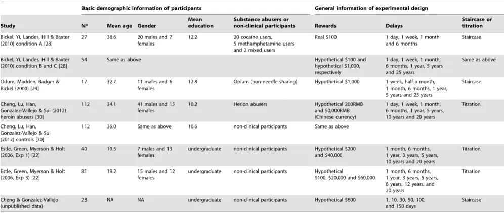
Previous research on intertemporal choice used aggregate (i.e. group) data or individual data to test model fitting (e.g. [8,25]). Because mathematical representations of behavior on the aggre-gate level may not reflect individual level behavior [26,27], we sought data that would allows us to fit the models at the level of each individual in each condition tested (i.e. indifference curve level). Data were obtained from published and unpublished sources (see Table 1) and the study fitted the models toN= 471 indifference curves.
Based on these criteria and a literature search, we contacted seven authors who had several publications and three of them provided us with the data from those publications (the data were chosen by those authors). In addition, we included data from our lab (one published and one unpublished set). We note that our inclusion criteria was not exhaustive of all studies on temporal discounting, because our aim was to both have a uniform set of studies (with similar methodologies) and enough data so that individual model fitting for both SA and NC was possible.
Table 1 details the characteristics of the studies [22,28–30] included in the present manuscript. Each study is described in terms of number of participants, age, gender, education level and drug type (if substance abusers). In describing each experimental design, we included the nature of the rewards (real or hypothet-ical), the magnitude of the rewards, the delays associated with the rewards and procedure of the task (staircase or titration). It should be noted again that the sample sizes described are not the number of participants. In some studies, one participant completed the temporal discounting tasks in more than one condition (e.g. different magnitudes). Therefore, sample size here indicated the number of actual discounting curves in each condition that was obtained from each of the different individuals. In other words, model fitting was performed at the level of each person’s curve. Fitting at discounting curve level allowed us to test if a parameter was able to capture the magnitude effect by comparing this parameter between different magnitude conditions within a same group of participants.
In order to easily identify the different studies in the text of this manuscript we label them using the authors’ names as found in Table 1 (from top to bottom): Bickel A, Bickel B, Bickel C, Odum, Cheng Heroin small, Cheng Heroin large, Estle 1 small, Estle 1
large, Estle 3 small, Estle 3 medium, Estle 3 large, Cheng control small, Cheng control large, and OU. The reader can easily find the testing conditions (e.g., whether the study was done with SA or NC; the size of the payoffs, etc.) by referring to Table 1. As seen in Table 1, there are a total of 14 studies.
Model fitting and Parametric Analyses
Indifference points were directly obtained from the studies. We note that in model fitting we maintained the time units used by the authors of the original studies. For example, although in [22] some delays were presented in years to participants the delays were transformed to months when fitting the Green-model by the authors. We followed the same procedure so that the delay units in our study were the same as those in the original studies. All models were fitted via non-linear regression on individual level using SPSS. The estimated parameters and goodness of fit results were checked for consistency, whenever possible, by comparing them to the results of the original studies when provided by the authors (this was the case for Odum [29]; and for Estle 1 and Estle 3 [22]). We compared the models by focusing on R2, but importantly, estimated parameters were examined with regards to meaningful-ness because models may fit data with nonsensical values. Further SA and NC groups were compared in terms of their parametric representations.
Results
Goodness of Fit Analyses
Table 2 and Table 3 list medianR2for all models in each study separating for studies having SA (Table 2) and for those having NC (Table 3). In each study, but Bickel condition B, theR2 of Figure 1. Subjective Value of A fromc-, Rachlin- with parametersk= 0.5 and 2;c= 1 and 10;s= 0.5. A = 100 and 1000.
doi:10.1371/journal.pone.0111378.g001
Testing Hyperbolic Models
base-model was lower than that of the other models, Wilcoxon Signed Rank Z$3.408,p-values,.01. In Bickel condition B, there was no difference in R2 between base-model and c-model, p -value..1. However, base-model fitted more poorly when com-pared to Rachlin- and Green-models in this study, Wilcoxon Z$
3.629,p-values ,.01. TheR2 differences between the base (one parameter) and the other models (two parameters) were not surprising, however, as a model with more parameters was expected to fit better and in general the base-model fitted well (medianR2= .881 across all studies).
To further test whether adding a parameter to the base-model was useful, we compared the models using a statistics that penalizes model for being over-parameterized. Schwarz Bayesian Criteria (SBC) is a measure of model selection derived by modifying the Bayesian information criterion [31]. It reflects the posterior probability of a specific model being the true model based on the observed data. SBC makes a trade-off between variance that can be accounted for and the complexity of the models. A model with smaller SBC is favored because it explains sufficient variance (compared to competing models) in a relative concise manner; if models provide equal fit from the perspective of variance accounted for, SBC penalizes the model with more parameters.SBCwas computed for each model in each study by first obtaining the median indifference points across participants, then fitting the models to these values. In each case, SBC=n * ln(SSE/n) +p * ln(n), where n was the number of median indifference points corresponding to the number of time delays, SSE was the residual variance, and p was the number of parameters. Results showed thatSBCfrom base-model was larger thanSBCfrom any two-parameter model in each study. Across all
the studies, meanSBC for base-model, c-model, Rachlin-model and Green-model were 60.2, 50.9, 46.8, and 49.2, respectively. Thus, the Rachlin-model fitted best from this perspective.
We proceeded to compare the medianR2values between two-parameter models using the Wilcoxon Signed Rank Z test. First, Rachlin- and Green-models did not show a difference in 10 out of 14 studies,p-values..1. In four conditions in [30], Rachlin-model fitted better,p-values,.05. Second, Rachlin-model was superior to thec-model in 8 out of 14 studies (Bickel B, Cheng heroin large, Estle 1 large, Estle 3 all three magnitude conditions, Cheng control small, and OU), p-values ,.05, and marginally better in two studies (Cheng heroin small and Estel 1 small), p-values ,.1. When comparing c- and Green-models, the Green-model was significantly better in 6 out of 14 studies (Bickel B, Cheng heroin large, Estle 1 large, Estle 3 all three magnitude conditions), p-values,.05, and marginally better in one study (OU),p-value,
.1. Hence, the Rachlin-model tended to provide better fits than the c-model, but only slightly better fits than the Green-model. This is consistent with the simulation results found in Figures 1 and 2 showing that the Rachlin- and Green-models tend to overlap.
We further compared the median R2 of the two-parameter models for SA and NC, respectively, across all of the studies. We note that the studies were not combined in this analysis as each person’s set of data was fitted individually. To the extent that a model was fitted at this micro-level, all specifics of the study were assumed to be reflected in the estimated parameter values. Table 4 displays the medianR2for each model in SA and NC.
In both populations, Rachlin-model had the highest medianR2. Green-model took the second place andc-model had the lowest fit Figure 2. Rachlin- and Green-Models with varying parameterss= 0.5 and 1.5;k= 0.5 and 2. A = 100 and 1000.
Table 1.Demographic Information of Participants and Experimental Design.
Basic demographic information of participants General information of experimental design
Study N* Mean age Gender
Mean education
Substance abusers or
non-clinical participants Rewards Delays
Staircase or titration
Bickel, Yi, Landes, Hill & Baxter (2010) condition A [28]
27 38.6 20 males and 7
females
12.2 20 cocaine users, 5 methamphetamine users and 2 mixed users
Real $100 1 day, 1 week, 1 month and 6 months
Staircase
Bickel, Yi, Landes, Hill & Baxter (2010) condition B and C [28]
54 Same as above Hypothetical $100 and
hypothetical $1,000, respectively
1 day, 1 week, 1 month, 6 months, 1 year, 5 years and 25 years
Same as above
Odum, Madden, Badger & Bickel (2000) [29]
17 32.7 11 males and 6
females
12.8 Opium (non-needle sharing) Hypothetical $1,000 1 week, half a month, 1 month, 6 months, 1 year, 5 years and 25 years
Staircase
Cheng, Lu, Han,
Gonzalez-Vallejo & Sui (2012) heroin abusers [30]
112 34.1 41 males and 15 females
10.2 Herion abusers Hypothetical 200RMB
and 50,000RMB (Chinese currency)
1 day, 1 week, 1 month, 6 months, 1 year, 5 years, 10 years and 20 years
Titration
Cheng, Lu, Han, Gonzalez-Vallejo & Sui (2012) controls [30]
112 36.0 Same as above 10.6 non-clinical participants Same as above
Estle, Green, Myerson & Holt (2006, Exp 1) [22]
40 19.5 7 males and 13
females
undergraduate non-clinical participants Hypothetical $200 and $40,000
1 month, 6 months, 1 year, 3 years, 5 years, 10 years and 20 years
Titration
Estle, Green, Myerson & Holt (2006, Exp 3) [22]
81 19.2 15 males and 12
females
undergraduate non-clinical participants Hypothetical
$100, $20,000 and $60,000
1 month, 6 months, 1 year, 3 years, 5 years, 8 years, 12 years, and 20 years
Titration
Cheng & Gonzalez-Vallejo (unpublished data)
28 NA NA undergraduate non-clinical participants Hypothetical $600 1, 10, 30, 50, 100,
and 150 days
Staircase
*: The number of actual discounting curves in each condition that was obtained from different individuals. doi:10.1371/journal.pone.0111378.t001
Testing
Hyperbolic
Models
PLOS
ONE
|
www.ploson
e.org
6
November
2014
|
Volume
9
|
Issue
11
|
among the three, all p-values ,.01, but again all models demonstrated excellent fit (medianR2
..93).
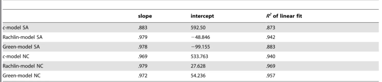
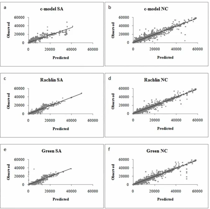
Another way of examining the predictive validity of the models was to perform a linear regression with predicted and observed values as the predictor and the criterion, respectively. A perfect prediction would result in a line with slope equal to one and an intercept equal to zero. This analysis was conducted using each person’s observed and predicted values and Figure 3 depicts the scatter plot of predicted and observed indifference points and the linear fits for each model in SA and NC. Table 5 providesR2s, slopes, and intercepts of the linear fits in Figure 3. In both populations, the linear fit of Rachlin-model was closest to the optimal values; Green andc-models followed (we note that we kept outliers in this analysis so that all models had the same number of observations). Taken together, all analyses indicated that Rachlin-model provided the best fit.
Analyses of Estimated Parameter Values
As is well known in the mathematical psychology literature, models may fit well but with non-interpretable parameters. Therefore, analysis with modeling must be concerned not only with fitting, but also with the meaningfulness of the parameters obtained [32]. We proceeded to examine outliers in the estimated parameters in order to gain a better sense of the performance of the models. We looked for very strange parameter values that could not be interpretable. For example, a participant had estimated parameters of k and s from Green-model equal to 5.661011and.0711, respectively. The extremely large value fork
in this case implies an indifference curve that drops immediately after the intercept A and remains essentially flat in the range of values of D studied. Instead of adopting conventional mean 6
3SD to detect outliers, we used this rather conservative approach to select outliers (i.e., selecting extremely large or extremely small estimated values), and found that across all studies, only 11 cases (out of 472, or 2.33%) were found to have outliers forc-model. The Rachlin-model had 4 cases (0.85%); and Green-model had 22 cases (4.66%). The cases identified by this procedure also had very lowR2s (R2#.201). Because the outlying cases constitute a very small percentage of the data, we keep them in all of the analyses except when focusing on the interpretation of mean parameter values as will be noted. We performed all previously reported group analyses by taking the outliers out and the conclusions remained unchanged.
The analyses with SBC revealed that the two-parameter models improved model fitting beyond simply increasing model complex-ity. We proceeded to test the specific values of the estimated parameterscandsin order to better understand the contribution they make to the base-model because whenc(a) =s= 1 the models reduce to the base-model. Table 6 shows the median and mean values of the parameters for each model in each study. We note
that values in Table 6 were calculated without the outliers. Doing so had little impact on medians, but was important in interpreting the mean values.
As shown in Table 6, in all studies the median and meancwere greater than 1. In terms of thec-model’s alternative representa-tions, this implies thata,1 (ord.0; seec-model descriptions). The median and meanswere smaller than 1 with two exceptions for mean Rachlin-s and four exceptions for mean Green-s. Table 7 further displays the percentage of the parameter values that were above (forc) or below (fors) the default value of 1 in each study. As shown in Table 7, forc-and Rachlin-models, 11 out of 14 (78.6%) studies showed that the new parameters were different from 1. For Green-model, 10 out of 14 (71.4%) displayed such a pattern. Binomial test showed that a significant proportion of the values were above or below the target value of 1.
Relationship Between Estimated Parameters and Discount Tendency
Previous studies using the Rachlin-model and/or Green-model [8,22–24] did not examine a possible association between the parameters, but it may be useful to do so in order to understand their behavior in representing discount tendency. Given the non-normal distributions and the few outliers, and in order to keep the number of data points constant for all models, we adopted Spearman rank correlation for these analyses without deleting observations. Table 8 shows the Spearman rank correlations between the two parameters in each model in each study.
As seen in Table 8, there is a general negative relationship between parameters k and s in Rachlin- and Green-models. A larger k in both models led to a greater devaluation whereas a smallersreduced this trend. Theoretical analyses of the function forms (Figure 2) show thats regulates the inflection and slope of the curves whereaskis more closely related to the general base level of discounting. Thus, the negative correlations betweenkand sindicated that these parameters tended to counteract their impact on discounting, allowing the functions to have greater flexibility. In contrast, parameters c and k in the c-model behaved more independently; with c determining the base level of discounting and k further adjusting the curvature of the subjective value function over time as shown in Figure 1.
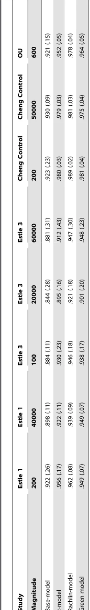
In order to further explore the relationship of the observed discounting and the estimated parameters, we used the area under the curve (AUC) as a parameter-free measure of the discounting tendency. AUC is a non-parametric measure adopted by [33], which is based on adding the segments enclosed by the empirically obtained indifference curve. AUC is standardized and thus ranges from 0 to 1. A larger AUC indicates that the participants discount future outcome to a lesser extent, whereas a smaller AUC represents higher discounting. We note that theoretically, the area under a curve is the integral of the function used to represent Table 2.Median R2for SA Group in Each Study.
Study Bickel A Bickel B Bickel C Odum Cheng Heroin Cheng Heroin
Magnitude 100 100 1000 1000 200 50000
Base-model .000 (.88) .753 (.90) .471 (.90) .777 (.81) .855 (.78) .829 (.77)
c-model .817 (.76) .753 (.90) .840 (.50) .921 (.28) .959 (.05) .884 (.09)
Rachlin-model .700 (.66) .882 (.40) .853 (.57) .940 (.11) .964 (.03) .967 (.04)
Green-model .848 (.89) .855 (.55) .859 (.68) .945 (.16) .941 (.06) .963 (.08)
discounting. This integral depends on the model parameters and in some cases, for Rachlin-model for example, the close form is quite complex. It is beyond of the scope of this paper to present a detailed analysis of such definite integrals, but suffice it to say that in general for these models the integral is inversely proportional to
k. Thus, to the extent that the models are close approximations to the data, we expect that the relationship betweenkand AUC to be negative.
Table 9 shows Spearman rank correlations between AUC and parameters in each study. Table 9 shows that thekparameters in base-model andc-model were highly negatively related with AUC. The pattern was more varied for Rachlin- and Green-models. The
kin Rachlin-model was significantly and negatively related with AUC in 9 out of 14 studies (64.3%). In contrast,kwas related with AUC in only three studies in the Green-model (21.0%). The parameter s was significantly correlated with AUC in 9 studies (64.3%) in each of Rachlin and Green-models. In all, but the heroin and control participants in [30], the significant relation-ships betweensand AUC were also negative.
In order to better understand the independent contribution of the parameters in predicting the discounting behavior as measured by AUC, partial Spearman rank correlations between AUC and a single parameter when controlling for the other were obtained. Table 10 displays these partial correlations.
Results in Table 10 show that in thec-model, the parameterk
was negatively associated with AUC after controlling for c. In contrast,cdid not reveal a consistent relationship with AUC in the presence ofk. This is consistent with model analyses (Figures 1) as c sets the base level of subjective value independently of delay, whereaskaffects subjective value via the weighting of delay. In Rachlin- and Green-modelskandswere significantly negatively related with AUC after controlling for the other parameter, which further demonstrated their more complex relationship in deter-mining subjective value as exhibited in Figures 1 and 2. In addition, the net relationship between AUC andk,orswas also negative in [30]. Hence, in thec-model,kuniquely described the AUC. Whereas in Rachlin- and Green-models, both k and s related to AUC with a greater k (ors) being associated with a smaller AUC (i.e., greater discounting).
Analysis of the Magnitude Effect
The magnitude effect refers to the phenomenon that greater discounting is observed for smaller than for larger gains [22]. This effect is due to changes in the conditions (payoff level) and provides additional tests of models’ parameters. In particular, the parameter shas been described as a person measure [24] and hence would not be expected to change with conditions. Thek parameter of Green- and the base-model has often been used to describe individual differences as earlier described, but it has also been used to describe changes due to situations (e.g., to account for sign and magnitude effects [25,30]); hence, the meaning of k may be broader to account for both person and situation based variability. Thecparameter is directly indexing a valuation process and hence it is expected to vary with payoff level. We examine these possibilities in tests of the magnitude effect.
We tested the effect in studies that contained a within-subjects manipulation of payoff size: Bickel B (A = 100) vs. Bickel C (A = 1000); Cheng heroin small (A = 200) vs. Cheng heroin large (A = 50000); Cheng control small (A = 200) vs. Cheng control large (A = 50000); Estle 1 small (200) vs. Estle 1 large (A = 40000); Estle 3 small (A = 100) vs. Estle 3 medium (A = 20000); Estle 3 small (A = 100) vs. Estle 3 large (A = 60000); and Estle 3 medium (A = 20000) vs. Estle 3 large (A = 60000). In [28], the magnitude effect was not reported and we found that there was no difference
Table 3. Median R 2 for NC Group in Each Study. Study Estle 1 E stle 1 E stle 3 E stle 3 E stle 3 Cheng Control Cheng Control O U Magnitude 200 40000 100 20000 60000 200 50000 600 Base-model .922 (.26) .898 (.11) .884 (.11) .844 (.28) .881 (.31) .923 (.23) .930 (.09) .921 (.15) c -model .956 (.17) .922 (.11) .930 (.23) .895 (.16) .912 (.43) .980 (.03) .979 (.03) .952 (.05) Rachlin-model .962 (.08) .939 (.09) .946 (.18) .921 (.18) .947 (.30) .989 (.02) .981 (.03) .978 (.04) Green-model .949 (.07) .949 (.07) .938 (.17) .901 (.20) .948 (.23) .981 (.04) .975 (.04) .964 (.05) Note: Numbers in p arentheses are the interquartile range. doi:10.1371/journal.pone. 0111378.t003
Testing Hyperbolic Models
in AUC between condition B (mean AUC = .431) and condition C (mean AUC = .398), pairedt(26) = .91,p= .37. In [30], the authors reported that there was a magnitude effect in both heroin participants and controls. In [22], it was found that the magnitude effect existed in all comparisons listed above except when comparing medium and large magnitudes in Experiment 3.
For studies in which the magnitude effect was not revealed by mean AUC changes, no changes of parameters were observed in any of the tests conducted. For the studies with magnitude effects, Wilcoxon Signed Ranked on parameter values within each study showed thatkfrom all models was able to reflect this effect with smaller values in the large than in the small magnitude conditions, all p-values #.05. In terms of parameter c, it reflected the magnitude effect in all studies (p-values #.01), but in Cheng control participants and Estle 1. Similar tok,cwas smaller in the large than in the small magnitude conditions. Note thatccan be expressed in terms ofain thea-model and thus it is of particular interest to analyze whether theaparameter is constant, or whether it changes with magnitude depicting intrinsic changes in subjective valuation due to payoff size. We proceeded to analyze the magnitude effect in terms of the parameteraby first estimating it at each curve level and confirming its relationship with c. Wilcoxon Signed Ranked test on parameter a for each study showed thataindexed the magnitude effect in all studies with a smaller ain the small magnitude conditions, all p-values ,.05. Parametric tests (paired samplest-test) on mean parameter values replicated these results with the following exceptions:kparameter of Green-model did not show an effect in [30];aparameter did not show an effect in the Estle 1 study.
In terms ofs, using Rachlin-model the changes were sometimes in the direction of the magnitude effect (i.e., smallersin the large than the small payoff condition) but other times the change was in the opposite direction. In Estle 3 (small vs. large; small vs. medium), the parametersshowed an opposite magnitude effect:s was greater in the large than in the small magnitude conditions,p -values,.05. There was no change ofsin Estle 1 between the two magnitude conditions,p-value..1. In Cheng control and heroin groups the direction of the magnitude effect was not consistently
shown by parameters, and the parameter values did not change significantly.
Parameter s in Green-model showed that it changed signifi-cantly with magnitude in both Cheng heroin participants and control participants in the direction of the effect,p-values,.01. The change was in the opposite direction in Estle 3 when comparing the small and large magnitude conditions,p,.05, but no effect when comparing the small and medium conditions. Similarly, there was no effect ofsin Estle 1 when comparing small and large conditions.
Taken together,k,canda, varied consistently in the direction of the magnitude effect with smaller values in conditions with larger A. In contrast,sdid not show a consistent pattern and this may be in agreement with the expectation thats must remain constant because it was to reflect an individual level tendency [24]. In order to further clarify the extent to which each parameter moved in the predicted direction, we computed the effect size (Cohen’s d) in each study. Following the methods provided by [34], weighted average dacross the studies were obtained along with its 95% confidence interval. The results appear in Table 11.
Table 11 shows that the 95% CIs include the value of zero only for the effect of the s parameter in both Rachlin- and Green-models. Although the sample size made the conclusions from this meta-analysis tentative (we have five studies demonstrating the magnitude effect), it was safe to say that there was no evidence of a consistent magnitude effect with parameters. This lends support to the assumption that s should remain constant with changes in contexts, but further studies are needed to clarify its role in describing context effects.
Parameter Comparison between SA and NC in an Experimental-Control Design
The groups of SA and NC participants come from different studies and conditions; therefore direct comparisons of parameter values is limited. Among these studies, however, [30] has both heroin-dependent patients and controls, and the groups were globally matched on age, gender, education, and income (for more details refer to [30]). Focusing on participants in this study, we Table 4.Median R2Within SA and NC.
SA NC
c-model .906 (.192) .960 (.070)
Rachlin-model .953 (.119) .971 (.058)
Green-model .937 (.133) .964 (.073)
doi:10.1371/journal.pone.0111378.t004
Table 5.Linear Regression of Predictive Validity of Models in SA and NC.
slope intercept R2of linear fit
c-model SA .883 592.50 .873
Rachlin-model SA .979 248.846 .942
Green-model SA .978 299.155 .883
c-model NC .969 533.763 .940
Rachlin-model NC .979 27.628 .969
Green-model NC .972 54.236 .957
compared the parameter values keeping study conditions separate (i.e., small and large magnitude conditions). The mean and median parameter values are found in Table 6, but to facilitate reading of the results, we present them in Table 12.
In terms of mediancandk, they were larger in SA than in NC in both small and large magnitude conditions, both Mann-Whitney testp-values,.01. In Rachlin- and Green-modelskwas larger in SA than in NC, and the reverse was true for s in all conditions, all Mann-Whitney testp-values ,.01. Therefore, the parameterkin all models indexed the difference between SA and NC in both magnitude conditions; so did thecparameter and both parameters moved in the expected direction, i.e., they were smaller in NC participants. Parameterafroma-model performed similar to parameterc: awas significantly smaller in SA than in NC. Thesparameter, on the other hand, moved in the opposite direction with smaller values for the SA individuals. As seen in
Figure 2, greater s implies greater discounting which would be expected for the SA participants instead.
There are limitations to using non-parametric tests when making comparisons because the magnitude of the quantities being compared is lost. Hence we performed tests of mean differences between the SA and NC groups. In order to conduct these tests, we identified the outliers by the procedure earlier described. We also assessed departures from symmetry of the distributions and transformed them using the natural log function when needed.
Independentt-tests were performed for each parameter between heroin-dependent and the non-clinical groups. For c-model, parameterkwas larger in SA than in NC in the small magnitude condition, t(110) = 5.24, p,.001, and in the large magnitude condition, t(109) = 5.17, p,.001. Parameterc was also larger in SA in both small and large magnitude conditions, t(110) = 5.11, p,.001 andt(109) = 5.0,p,.001, respectively.
Figure 3. Scatter Plots of Predicted and Observed Indifference Points for Each Model in each SA and NC Groups. doi:10.1371/journal.pone.0111378.g003
Testing Hyperbolic Models
c-model Rachlin-model Green-model
k c k s k s
Bickel ASA Median .004 (.03) 1.133 (.50) .096 (.43) .257 (.60) 1.251 (6.9) .273 (.43)
Mean .020 (.03) 1.589 (1.3) .456 (1.0) .474 (.63) 15.14 (29.4) 1.651 (4.68)
Bickel BSA Median .002 (.009) 1.092 (.20) .041(.13) .486 (.55) .040 (.613) .252 (.44)
Mean .058 (.009) 2.839 (8.46) 1.468 (7.2) .603 (.51) 4.564 (10.9) .307 (.27)
Bickel CSA Median .002 (.009) 1.092 (.38) .066 (.24) .423 (.49) .178 (1.6) .288 (.59)
Mean .030 (.08) 1.330 (.83) .269 (.67) .604 (.91) 5.112 (16.1) .399 (.36)
OdumSA Median .013 (.641) 1.067 (.32) .259 (2.4) .980 (1.6) 3.97(10.7) .175 (85)
Mean 2.41 (6.81) 1.511 (1.53) 3.089 (7.8) 1.438 (1.5) 10.27 (16.2) .483 (.50)
Cheng Heroin smallSA Median .008 (.007) 1.276 (.35) .117 (.24) .512 (.27) .122 (.72) .333 (.17)
Mean .010 (.01) 1.527 (.91) .270 (.43) .556 (.19) 1.965 (5.25) .382 (.20)
Cheng Heroin largeSA Median .002 (.002) 1.151 (.23) .051 (.11) .520 (.23) .047 (.23) .286 (.13)
Mean .002 (.001) 1.292 (.39) .153 (2.7) .539 (.32) .754 (3.25) .260 (.12)
Estle 1 smallNC Median .054 (.10) 1.058 (.39) .193 (.42) .867 (.56) .268 (1.30) .767 (.71)
Mean .109 (.19) 1.202 (.40) .265 (.42) .878 (.47) 1.122 (2.5) .694 (.41)
Estle 1 largeNC Median .009 (.02) 1.032 (.07) .024 (.07) .774 (.37) .035 (.15) .419 (.76)
Mean .040 (.09) 1.046 (.13) .070 (.11) .864 (.38) .150 (.266) .920 (1.7)
Estle 3 smallNC Median .051 (.17) 1.192 (.38) .205 (.20) .641 (.43) .549 (1.15) .439 (.52)
Mean .114 (.16) 1.270 (.37) .316 (.32) .705 (.27) 1.106 (.25) .694 (.63)
Estle 3 mediumNC Median .007 (.02) 1.026 (.08) .020 (.03) .871 (.45) .027 (.12) .550 (.87)
Mean .013 (.02) 1.056 (.10) .037 (.06) .834 (.38) .508 (1.84) 3.76 (13.3)
Estle 3 largeNC Median .006 (.02) 1.019 (.13) .012 (.05) .846 (1.04) .019 (.27) .732 (37.4)
Mean .013 (.01) 1.072 (.16) .066 (.10) 1.004 (.61) .344 (1.2) 17.40 (26.1)
Cheng Control smallNC Median .004 (.002) 1.040 (.07) .012 (.02) .808 (.20) .009 (.01) .653 (.22)
Mean .005 (.004) 1.088 (.16) .043 (.01) .789 (.17) .187 (.95) .586 (.23)
Cheng Control largeNC Median .001 (.0004) 1.061 (.06) .008 (.01) .663 (.20) .005 (.005) .381 (.19)
Mean .0009 (.0005) 1.067 (.06) .014 (.02) .753 (.27) .008 (.06) .535 (1.2)
OUNC Median .008 (.01) 1.036 (.09) .014 (.04) .844 (.44) .008 (.02) .525 (1.61)
Mean .011 (.01) 1.056 (.08) .041 (.06) .832 (.30) .079 (.23) 3.045 (7.2)
SA Median .003 (.009) 1.157 (.34) .086 (.26) .503 (.38) .120 (4.07) .282 (.31)
Mean .346 (2.74) 1.645 (3.06) 3.078 (9.8) .419 (1.36) .754 (3.9) .958 (4.7)
NC Median .004 (.015) 1.043 (.95) .016 (.05) .771 (.34) .012 (.09) .465 (.54)
Mean .041 (.23) 1.099 (.21) .355 (1.35) 1.742 (6.2) .086 (.19) .827 (.35)
Testing
Hyperbolic
Models
ONE
|
www.ploson
e.org
11
November
2014
|
Volume
9
|
Issue
11
|
For Rachlin-model, parameter k demonstrated the group difference in both magnitude conditions, t(110) = 7.20, p,.001, andt(104) = 7.38,p,.001, respectively. Parameters, however, was smaller in SA than in NC in small and large magnitude conditions, witht(110) =27.20,p,.001 andt(110) =25.28,p,.001, respec-tively.
Similar to the other models, in Green-model, SA displayed a largerkwhen compared to NC,t(107) = 3.42,p= .001 in the small magnitude condition;t(105) = 2.38,p,.05 in the large magnitude condition. Parameter s moved in the opposite direction of parameterk. In each case, swas smaller in SA:t(104) =26.024, p,.001 in the small condition; t(110) =24.013, p,.001 in the large condition. Thus, in agreement with the non-parametric tests the parameters k and c consistently represented the group differences whereas the parametersdid not.
Discussion
The present study aimed to better understand the basis of the observed discounting behavior of both substance abusers and non-clinical individuals. Traditionally the single parameter model of Equation 1 has been used to describe group differences with parameterkbeing on average greater for the substance abusers than for the non-clinical individuals. Our results replicate these findings. However, thekparameter is too general and differences in discounting tendency may be due to valuation process differences, or to time perception distortions that in turn affects the subjective value of a future amount. The present study sought to clarify the psychological basis for discounting in intertemporal choice and the observed group differences using a modeling approach. The models tested represent valuation, time perception, and general time/amount scaling functions: c-, Rachlin-, and Green-models, respectively. Rachlin- and Green-models have been widely used with substance abusers and hence served as benchmarks for investigating individual differences. Thec-model, as it derives from thea-model, has been theoretically considered but not tested. This study advances our understanding of the manner in which models of discounting behavior represent different psychological process for different individual and conditions.
The analyses first elucidated the similarities and differences of the function forms and how model parameters produce varying discounting tendencies for different A and D levels. Through such simulations, it was shown that Rachlin- and Green-models predicted very similar discounting for a wide array of delays. In contrast, the base-model, and c-model with greater c.1, can produce deeper discounting patterns than the Rachlin- and Green-models at a fixed k. Furthermore, the analyses demon-strated the different roles ofkin the different models. Inc-model,
khad a greater influence in regulating the shape of the discounting curve, whereas c set the overall base-level of discounting. In contrast, in Rachlin- and Green-models, parametersappeared to regulate the changes of subjective value over time withkserving to set the base level of discounting. However, the relationship betweenkandswas very interactive; a largescould counteract a smallkand vice versa. Results of the simulation also demonstrated that A affected the rate of discounting (change in subjective value per unit of time).
Moreover, discounting rate is not constant throughout the delay periods and this implies that individuals are more sensitive to delay differences closer to the present moment than later. Tests of such implications are needed to further study the models’ validity. For example, assume a participant has estimatedk= 0.08 ands= 0.5 and let us use the Rachlin-model without loss of generality. The
Table 6. Cont. c -model Rachlin-model Green-model kc k s k s Total Median .004 (.01) 1.071 (.21) .032 (.14) .646 (.40) .024 (.16) .347 (.44) Mean .173 (1.82) 1.278 (1.99) .382 (2.61) .725 (.52) .468 (1.37) .865 (3.24) Note: Numbers in parentheses are IQR and standard deviation for median and m ean values, respectively. SA: m edian and m ean of parameter values compute d across all cases in studies having substance abusers; NC: median and mean of parameter values computed across all cases in studies having non-clinical participants. The Total has the median and m ean computed across all cases and studies. When SA and NC are superscripts, they indicate whether the study contains substance abusers or non-clinical people. doi:10.1371/journal.pone. 0111378.t006
Testing Hyperbolic Models
model predicts a subjective value of 798.09 for the option (A = 1000, D = 10) and a value of 736.5 for (A = 1000, D = 20); this is a 61.59 drop in subjective value of A in a period difference of 10 D units. In later periods (between D = 20 and D = 30) the drop in
subjective value of A is of 41.17. This implies that the preference for the sooner option would be stronger in the first than in the second comparison. However, it is likely that by dominance a decision maker confronted with such pairs of options would select Table 7.Percentage of Deviation of Parameters From The Value of 1 in Each Study.
c.1 (%) Rachlin-s,1 (%) Green-s,1 (%)
Bickel ASA 85*** 93*** 85**
Bickel BSA 85*** 89*** 81**
Bickel CSA 81*** 93*** 89**
OdumSA 65 53 65
Cheng Heroin smallSA 96*** 98** 100***
Cheng Heroin largeSA 80* 75* 75*
Estle 1 smallNC 70 60 70
Estle 1 largeNC 80* 75* 75*
Estle 3 smallNC 81** 85** 85**
Estle 3 mediumNC 78** 74* 67
Estle 3 largeNC 63 59 56
Cheng Control smallNC 88*** 91*** 100***
Cheng Control largeNC 84*** 89*** 93***
OUNC 82** 71* 71*
SA 89*** 92*** 90***
NC 80*** 82*** 79***
Total 84*** 84*** 86***
Note: *p,.05; **p,.01; ***p,.001. SA: percentage computed across all cases in studies with substance abuse individuals; NC: percentage computed across all cases in studies with non-clinical individuals. Total: percentage computed across all cases in all studies. When SA and NC are superscripts, they indicate whether the study contains substance abusers or non-clinical people.
doi:10.1371/journal.pone.0111378.t007
Table 8.Spearman Rank Correlations Between the Model Parameters.
c-model (k,c) Rachlin-(k,s) Green-(k,s)
Bickel ASA .181
2.239 2.505**
Bickel BSA
2.161 2.363 2.733***
Bickel CSA .204
2.243 2.541**
OdumSA
2.397 2.162 2.834***
Cheng Heroin smallSA .266*
2.845***
2.845***
Cheng Heroin largeSA
2.273*
2.977***
2.640***
Estle 1 smallNC
2.429 2.442 2.829***
Estle 1 largeNC
2.053 2.439 2.433
Estle 3 smallNC
2.266 2.447*
2.584**
Estle 3 mediumNC
2.041 2.597**
2.814***
Estle 3 largeNC
2.410*
2.808***
2.925***
Cheng Control smallNC .140
2.903***
2.353**
Cheng Control largeNC .492***
2.963***
2.374**
OUNC 0.0
2.822***
2.455*
SA .078 2.621***
2.494***
NC 2.018 2.408***
2.583***
Total 2.012 2.620***
2.555***
Note: *p,.05; **p,.01; ***p,.001. SA: correlation computed across cases in studies with substance abusers. NC: correlation computed across all cases in studies with non-clinical individuals. Total: correlation computed across all cases in all studies. When SA and NC are superscripts, they indicate whether the study contains substance abusers or non-clinical people.
Table 9.Spearman Correlations Between AUC and Estimated Parameters.
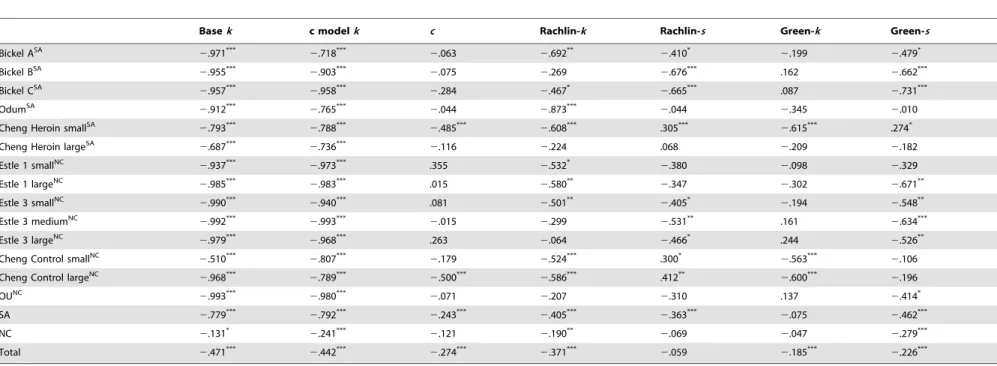
Basek c modelk c Rachlin-k Rachlin-s Green-k Green-s
Bickel ASA
2.971***
2.718***
2.063 2.692**
2.410*
2.199 2.479*
Bickel BSA
2.955***
2.903***
2.075 2.269 2.676*** .162
2.662***
Bickel CSA
2.957***
2.958***
2.284 2.467*
2.665*** .087
2.731***
OdumSA
2.912***
2.765***
2.044 2.873***
2.044 2.345 2.010
Cheng Heroin smallSA
2.793***
2.788***
2.485***
2.608*** .305***
2.615*** .274*
Cheng Heroin largeSA
2.687***
2.736***
2.116 2.224 .068 2.209 2.182
Estle 1 smallNC
2.937***
2.973*** .355
2.532*
2.380 2.098 2.329
Estle 1 largeNC
2.985***
2.983*** .015
2.580**
2.347 2.302 2.671**
Estle 3 smallNC
2.990***
2.940*** .081
2.501**
2.405*
2.194 2.548**
Estle 3 mediumNC
2.992***
2.993***
2.015 2.299 2.531** .161
2.634***
Estle 3 largeNC
2.979***
2.968*** .263
2.064 2.466* .244
2.526**
Cheng Control smallNC
2.510***
2.807***
2.179 2.524*** .300*
2.563***
2.106
Cheng Control largeNC
2.968***
2.789***
2.500***
2.586*** .412**
2.600***
2.196
OUNC
2.993***
2.980***
2.071 2.207 2.310 .137 2.414*
SA 2.779***
2.792***
2.243***
2.405***
2.363***
2.075 2.462***
NC 2.131*
2.241***
2.121 2.190**
2.069 2.047 2.279***
Total 2.471***
2.442***
2.274***
2.371***
2.059 2.185***
2.226***
Note: *p,.05; **p,.01; ***p,.001. SA: correlation computed across cases in studies with substance abusers. NC: correlation computed across all cases in studies with non-clinical individuals. Total: correlation computed across all cases in all studies. When SA and NC are superscripts, they indicate whether the study contains substance abusers or non-clinical people.
doi:10.1371/journal.pone.0111378.t009
Testing
Hyperbolic
Models
PLOS
ONE
|
www.ploson
e.org
14
November
2014
|
Volume
9
|
Issue
11
|
the sooner options with 100 percent certainty in both situations; thus show no reduced time sensitivity in choice. This means that the models’ predicted preferences may not agree with participants’ behavior once the models are tested with another method. More generally, cross-validation studies are much needed, and by this we mean that a function derived via the indifference point method-ology is then used to predict behavior outside of the data employed in model fitting.
In terms of model testing, the analysis inspected not only model fit and the corresponding proportion of variance accounted for, but also examined the meaning of the estimated parameters in different groups and in different magnitude conditions. Ultimately, it is the meaning of such parameters that can provide psycholog-ical understanding. First, compared to the base-model, all the two-parameter models improved fit non-trivially as demonstrated with the SBC measure and with the tests of mean and median
parameter values against the default value of 1. Among the two-parameter models, Rachlin-model displayed the best fit at the individual level in both SA and NC. This result contrasts with that of [8,23] finding that no difference was found between Rachlin-and Green-models. A possible reason for this difference was that a greater number of studies were included, with a wider range of D. We note, however, that all of the models performed extremely well when consideringR2, and that the function forms tend to overlap in many situations as shown in the function form analysis. Thus, not finding differences may be more the rule than the exception. In terms of estimated parameters, previous research found that the parametersin Green- and Rachlin-models was smaller than 1 [23]. We replicated this finding in fourteen studies. Additionally, we found that a significant proportion of cases had aclarger than 1 inc-model. Therefore, from the perspective of whether the two-parameter models may be easily reduced to the one-two-parameter Table 10.Partial Spearman Rank Correlations Between Model Parameters and AUC.
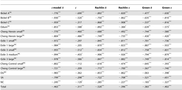
c-modelk c Rachlin-k Rachlin-s Green-k Green-s
Bickel ASA
2.776***
2.690***
2.892***
2.820***
2.477*
2.630**
Bickel BSA
2.930***
2.520**
2.750***
2.862***
2.635***
2.810***
Bickel CSA
2.959***
2.317 2.868***
2.908***
2.537**
2.816***
OdumSA
2.853***
2.588*
2.892***
2.384*
2.639**
2.573*
Cheng Heroin smallSA
2.770***
2.460***
2.688***
2.492***
2.744***
2.580***
Cheng Heroin largeSA
2.804***
2.486***
2.749***
2.735***
2.430**
2.420**
Estle 1 smallNC
2.972***
2.297 2.845***
2.811***
2.701**
2.736**
Estle 1 largeNC
2.984***
2.205 2.870***
2.823***
2.887***
2.933***
Estle 3 smallNC
2.955***
2.512**
2.834***
2.812***
2.758***
2.831***
Estle 3 mediumNC
2.994***
2.455*
2.906***
2.926***
2.794***
2.879***
Estle 3 largeNC
2.978***
2.586**
2.847***
2.882***
2.749***
2.814***
Cheng Control smallNC
2.802***
2.112 2.618***
2.474***
2.645***
2.393**
Cheng Control largeNC
2.721***
2.209 2.772***
2.700***
2.567***
2.740***
OUNC
2.983***
2.362 2.853***
2.862***
2.063 2.398*
SA 2.799***
2.298***
2.722***
2.708***
2.521***
2.651***
NC 2.245***
2.129*
2.285***
2.227***
2.183**
2.327***
Total 2.463***
2.311***
2.520***
2.396***
2.383***
2.402***
Note: *p,.05; **p,.01; ***p,.001. SA: correlation computed across cases in studies with substance abusers. NC: correlation computed across all cases in studies with non-clinical individuals. Total: correlation computed across all cases in all studies. When SA and NC are superscripts, they indicate whether the study contains substance abusers or non-clinical people. When SA and NC are superscripts, they indicate whether the study contains substance abusers or non-clinical people.
doi:10.1371/journal.pone.0111378.t010
Table 11.Meta-Analysis of Effect Size (Cohen’s d) When Testing Magnitude Effect.
Parameters Avg(d) SD(da
) 95% CI
c-modelk 0.851 0.472 [.415–1.29]
c 0.312 0.141 [.132–.492]
a-modelk 0.861 0.53 [.377–1.35]
a 0.616 0.273 [.343–.899]
Rachlin -k 0.39 0.0 [.283–.497]
Rachlin-s 20.087 0.529 [2.569–.395]
Green-k 0.317 0.035 [.184–.450]
Green-s 20.008 0.674 [2.613–.597]
Note. a: According to Hunter & Schmidt (2004), the population variance of effect size (d2
) is obtained by subtracting variance due to sampling error from observed variance adjusted by sample size.
base model, our results indicated that this was not the case. Psychologically, in terms of the valuation process,cbeing larger than 1 implies a power function for subjective value that is concave (i.e.,a,1 ina-model). This is consistent with the general value function of prospect theory and other utility functions that assume diminishing returns [15]. That the parameterswas also not equal to 1 echoed the notion that subjective time was different from objective time [19–21]. However, we note that havings,1 meant that time was not enhanced, but rather shrunk, and the fact thats was smaller in SA than in NC implied that the subjective delays were smaller for SA than NC. This contradicts the expectation that SA’s would overestimate the duration of time as reported in [20]. Indeed, more generallys,1 reduces discounting as observed in Figures 1 and 2, everything else constant. This means that the greater discounting observed in SA cannot be attributed to time perception processes in the manner represented bysin Rachlin-and Green-models. It is the compensation of a smaller s by a greater k that accounts for greater discounting in the SA individuals.
Another finding was that Rachlin- and Green-models produced estimated parameters that were statistically and negatively related to each other. This suggests that the models improved fitting in part by having parameters compensated for each other. As the function form analyses showed, the parameterscould counteract the effects ofkand vice versa. This was not so for the parameterc in thec-model. Furthermore, the models’ parameters showed that the parameters k and s were negatively related to AUC when controlling for the other, whereas this was not the case forc. In combination, this shows thatcis a less redundant parameter.
Additional analyses on contextual differences showed that the parameterk in all models was consistently greater in the small versus the large magnitude conditions, thus being able to describe themagnitude effect. The same was true in almost all cases for the cparameter and in all cases for the correspondingaparameter. In contrast, parameters in either the Rachlin- or the Green-model did not show a consistent pattern in relationship to the magnitude effect. These results reestablish that the k parameter may be conceived as a situation specific, or context effect index, but nots. In a similar vein, when testing models with data from heroin patients and control participants within a single study,kwas larger in the heroin group than in controls. This was also true for thec parameter. In contrast s was smaller for the substance abuse individuals than the non-clinical group. Hence, parameterskand c systematically measured the average individual tendencies, whereas s allowed for better model fit but its values did not advance additional meaning that could describe, or explain these person level effects.
Overall, we found that Rachlin-model provided the best description of the data across studies from the perspective of variance accounted for, followed by Green-model. This indicated that a time perception function (Rachlin-model), or a general amount-to-time scaling function (Green-model) was beneficial to the base model in explaining additional variance. However, both models have challenges with regards to the interpretation of their parameters. In particular, the finding that the SA individuals hads values that would result in less rather than greater discounting is problematic; model fitting was significantly improved withs, but psychological understanding was not. Furthermore thes param-eter negatively correlated withkwhich resulted in small changes in sthat counteracted the movements ofkacross the many studies reviewed. Thus,sadds flexibility to the models, but it does not add explanatory power to them. Further studies are needed to establish sas a person level index. In terms ofk, it described both context
Table 12. Median and Mean Values of the Parameters of Heroin and Control Participants in [30]. c -model Rachlin-model Green-model kc k s k s Heroin S Median .008 (.007) 1.276 (.35) .117 (.24) .512 (.27) .122 (.72) .333 (.17) Mean .010 (.01) 1.527 (.91) .270 (.43) .556 (.19) 1.965 (5.25) .382 (.20) Heroin L Median .002 (.002) 1.151 (.23) .051 (.11) .520 (.23) .047 (.23) .286 (.13) Mean .002 (.001) 1.292 (.39) .153 (2.7) .539 (.32) .754 (3.25) .260 (.12) Control S Median .004 (.002) 1.040 (.07) .012 (.02) .808 (.20) .009 (.01) .653 (.22) Mean .005 (.004) 1.088 (.16) .043 (.01) .789 (.17) .187 (.95) .586 (.23) Control L Median .001 (.0004) 1.061 (.06) .008 (.01) .663 (.20) .005 (.005) .381 (.19) Mean .0009(.0005) 1.067 (.06) .014 (.02) .753 (.27) .008 (.06) .535 (1.2) Note: Superscripts Sand Lindex small and large p ayoffs. Numbers in parentheses are IQR for median, and standard deviation for means; means computed without outliers. doi:10.1371/journal.pone. 0111378.t012
Testing Hyperbolic Models
![Table 1 details the characteristics of the studies [22,28–30]](https://thumb-eu.123doks.com/thumbv2/123dok_br/17319809.249690/4.918.92.831.96.544/table-details-characteristics-studies.webp)