Measuring Impatience in Intertemporal
Choice
Salvador Cruz Rambaud*☯, María José Muñoz Torrecillas☯
Departamento de Economía y Empresa, Facultad de Ciencias Económicas y Empresariales, Universidad de Almería, La Cañada de San Urbano, s/n, 04120, Almería, Spain
☯These authors contributed equally to this work.
Abstract
In general terms, decreasing impatience means decreasing discount rates. This property has been usually referred to as hyperbolic discounting, although there are other discount functions which also exhibit decreasing discount rates. This paper focuses on the measure-ment of the impatience associated with a discount function with the aim of establishing a methodology to compare this characteristic for two different discount functions. In this way, first we define the patience associated with a discount function in an interval as its corre-sponding discount factor and consequently we deduce that the impatience at a given moment is the corresponding instantaneous discount rate. Second we compare the degree of impatience of discount functions belonging to the same or different families, by consider-ing the cases in which the functions do or do not intersect.
Introduction
Impatiencewas already defined in 1960 by [1] as the decrease in the aggregate utility with respect to time. In his work, he stated:“this study started out as an attempt to formulate postu-lates permitting a sharp definition of impatience, the short term Irving Fisher has introduced for preference for advanced timing of satisfaction”([1] referred to the 1930 work of Fisher [2]:
“The Theory of Interest”(Chapter IV)). This idea of a preference for advancing the timing of future satisfaction has been used in economics since the appearance of Böhm-Bawerk’s work:
Positive Theorie des Kapitals[3].
Some authors use the termimpulsivityas a synonym of impatience, e.g. [4]. In effect, [5] define impulsivity in intertemporal choice as a“strong preference for small immediate rewards over large delayed ones”. We can find a similar and earlier definition in [6] who defined the impulsiveness (in choices among outcomes of behavior) as“the choice of the less rewarding over more rewarding alternatives”. Observe that impatience has usually been presented in rela-tive terms by comparing the values shown by two intertemporal choices. [7] states that the term impulsivity is often utilized in psychiatric studies on intertemporal choice and cites some examples of impulsive subjects such as smokers, addicts and attention-deficient hyperactivity-disorder patients. The opposite behavior to impulsivity is self-control.
a11111
OPEN ACCESS
Citation:Cruz Rambaud S, Muñoz Torrecillas MJ (2016) Measuring Impatience in Intertemporal Choice. PLoS ONE 11(2): e0149256. doi:10.1371/ journal.pone.0149256
Editor:Pablo Brañas-Garza, Middlesex University London, UNITED KINGDOM
Received:November 13, 2015
Accepted:January 30, 2016
Published:February 18, 2016
Copyright:© 2016 Cruz Rambaud, Muñoz Torrecillas. This is an open access article distributed
under the terms of theCreative Commons Attribution
License, which permits unrestricted use, distribution, and reproduction in any medium, provided the original author and source are credited.
Data Availability Statement:All data are shown in the paper.
Funding:This paper has been partially supported by
the project“Valoracion de proyectos
gubernamentales a largo plazo: obtencion de la tasa
social de descuento”, reference: P09-SEJ-05404,
Proyectos de Excelencia de la Junta de Andaluca and Fondos FEDER. The funders had no role in study design, data collection and analysis, decision to publish, or preparation of the manuscript.
As for the measure of impatience, the rate of discount is commonly taken to indicate the level of impulsivity or impatience in intertemporal choices. [8] offer an interesting review of the empirical research on intertemporal choice and summarize the implicit discount rates from all the studies they reviewed. In the same way, [9] and [10] provide a revision on time-declining discount rates from the observed individual choice, among other approaches.
But, as will be demonstrated in the next section, there are other ways to quantify the impa-tience. Our main objective in this paper is to develop a measure of the impatience exhibited by the discount function associated with the underlying intertemporal choice. In this case, we will be able to compare the impatience associated with two discount functions.
On this subject, there are many empirical papers trying to compare the degree of impatience of a group of individuals at different points in time (e.g. [11], [12], [13], [14]) or to compare the degree of impatience with different discount functions (e.g. [7], [13], [15], [16], [17], [18]). There is also an alternative measure of discounting: the area under the curve proposed by [19], which allows comparing the impatience between individuals in a model-free way (since it is not tied to any specific theoretical framework). See [20] for a review of this method and refer-ence to several studies in which it has been employed.
Another approach related to this topic is the analysis of the main types of impatience. Thus, when studying the impatience in intertemporal choice, we usually find that it decreases. Fol-lowing [21],decreasing impatienceimplies an inverse relationship between the discount rate and the magnitude of the delay and has usually been attributed tohyperbolic discounting. In the same way, [22] treats decreasing impatience as the core property which is parametrically expressed by hyperbolic and quasi-hyperbolic discount functions.
Recently, several studies have included different degrees of impatience and not only decreas-ing impatience ([23], [24], [25], [26], [27], [28]). [25] report individual evidence of lower dis-counting for intervals closer to the present than for distant ones, demonstrating concave discounting, which impliesincreasing impatience.
Additionally, a number of empirical papers have recently appeared which relate impatience with decision-making in games. For example, [29] study the relationship between impatience, risk aversion, and household income. [30] conducts a research on impatience, risk aversion, and working environment. [31] empirically study the patience/impatience of punishers in a multilateral cooperation game. In a similar vein, [32] explore the relationship between impa-tience and bargaining behavior in the ultimatum game.
In this paper the concept ofpatienceassociated with a discount function (F(t)) in an interval [t1,t2] is defined as the value of the discount factor corresponding toF(t) in this interval.
Hence, the impatience associated withF(t) in an interval will be calculated as 1 minus the dis-count factor associated with the given interval, which is the value of the disdis-count correspond-ing to $1 in this interval. Additionally, we present a procedure to compare the degree of impatience between two discount functions, of the same or different family. In [33] we find a comparison between exponential and hyperbolic discount functions controlling the overall impatience in order to isolate the differences due to self-control problems only. The controlled comparison is made by means of age adjustment which equalizes areas under discount functions.
The objective of this paper is interesting for the following reasons:
2. Inevitably, most researches on this issue show the discount functions which, in each case, better fit the data. In effect, [34] estimate the parameters of the main intertemporal choice models: exponential, simple hyperbolic, quasi-hyperbolic, andq-exponential. Subsequently, they compare the impatience shown by two groups by simply comparing the discount rates of the corresponding discount functions. Obviously, this is not an accurate procedure because some discount functions are biparametric and so it should require a comparison of both parameters defining the function. Moreover, this is a simplification because it would be interesting to compare the impatience in a certain time interval where, among other cir-cumstances, the relative position of the impatience levels can change. Even the use of theq -exponential discount function assumes working with an -exponential, a hyperbolic or a gen-eralized hyperbolic discount function, depending on the concrete values ofqandkq.
There-fore, the most important thing is to obtain the discount function which better fits the collected data, and then it is likely that the subsequent comparison can involve discount functions belonging to different families. Even the comparison between two discount func-tions belonging to the same family (for instance, two hyperbolic discount funcfunc-tions) is also noteworthy because they usually exhibit different parameters.
3. Several researches have considered the impatience shown by individuals of different nation-alities, genders or socio-economic levels. The comparison of the discount functions involved in these studies is important in order to design, for example, a market segmentation strategy according to the former criteria.
[35] state that the intertemporal impatience can be applied to the acquisition of material objects instead of money. This makes the issue of impatience very interesting in marketing and consumer behavior. They point out some culture-related differences between western and eastern participants in the empirical study conducted by them: the former valued immediate consumption more than the latter. In the same way, [14] experimentally com-pared intertemporal choices for monetary gains and losses by American and Japanese sub-jects, demonstrating that Westerners are more impulsive and time-inconsistent than Easterners. [36] also recognize the accuracy of discounting to explain impatience in market-ing.
Finally, [37] have found that gender and autobiographical memory can have an effect on delay discounting: there is a significant difference between men and women because, in the case of higher memory scores, the former showed less impatience when discounting future rewards. In the experimental analysis, they used the standard hyperbolic and the quasi-hyperbolic models.
It is therefore apparent that the comparison of discount functions will be of interest to seg-ment a market depending on the impatience exhibited by individuals who are classified by different criteria (geographical, gender, culture, etc.).
This paper is organized as follows. After this introduction, in Section 2 we will formally define the impatience (impulsivity) ranging from the discount corresponding to $1 in an inter-val [t1,t2] (a two-parameter function, referred to asimpatience-arc) to the instantaneous
Defining impatience (impulsivity) in intertemporal choice
In economics and other social sciences it is common practice to try to simplify the complexity of the models describing the behavior corresponding to a group of people. This is the case of discount functions in the framework of intertemporal choice within the field of finance. In effect, a (dynamic) intertemporal choice can be described by atwo-variable discount function
([38]), that is, a continuous function
F:RRþ !R
such that
ðd;tÞ7!Fðd;tÞ;
whereF(d,t) represents the value atd(delay) of a $1 reward available at instantd+t. In order to makefinancial sense, this function must satisfy the followingconditions:
1. F(d, 0) = 1,
2. F(d,t)>0, and
3. For everyd,F(d,t) is strictly decreasing with respect tot.
A discount function is said to be
1. With bounded domainif, for everyd2R, there exists an instanttd2Rþ, depending ond,
such thatF(d,td) = 0.
2. With unbounded domainif, for everyd2Randt2Rþ, one hasF(d,t)>0. Within this
group, a discount function can be:
a. Regularif lim
t!þ1Fðd;tÞ ¼0, for everyd2R.
b. Singularif lim t!þ1
Fðd;tÞ>0, for everyd2R.
Regular discount functions are the most usual valuation financial tools. Nevertheless, and as indicated at the beginning of this Section, this discounting model can be simplified by using a functionF(t) independent of delayd. More specifically, aone-variable discount function F(t) ([38] and [39]) is a continuous real function
F:Rþ !R
such that
t7!FðtÞ;
defined within an interval [0,t0) (t0can even be +1), whereF(t) represents the value at 0 of a
$1 reward available at instantt, satisfying the following conditions:
1. F(0) = 1,
2. F(t)>0, and
3. F(t) is strictly decreasing.
Theorem 1. A discount functionF(t) gives rise to the total preorder≽defined by
ðC1;t1Þ ðC2;t2Þ if C1Fðt1Þ C2Fðt2Þ;
satisfying the following conditions:
1. Ift1t2, then (C,t1)≽(C,t2), and
2. IfC1C2, then (C1,t)≽(C2,t).
Reciprocally, every total preorder≽satisfying conditions (i) and (ii) defines a discount
function.
Theorem 1 shows that, in intertemporal choice, an agent can indistinctly use a discount function or a total preorder. In this way, the concept of impatience has been mainly treated with a total preorder. For example, [40] propose the following choice:“$10 in a year or $15 in a year and a week”. In this way, they state that:“If an individual A prefers the first option ($10 in a year) while B prefers the second option ($15 in a year and a week), it is said that A is more impulsive than B because A prefers a smaller, but more immediate reward, whereas B prefers to wait a longer time interval to receive a greater reward”. Nevertheless, our aim here is to define the concept of impatience by using discount functions. In effect, given a one-variable discount functionF(t), thepatienceassociated withF(t) in an interval [t1,t2] (t1<t2) is defined
as the value of the discount factorf(t1,t2) corresponding to this interval, viz:
fðt1;t2Þ:¼
Fðt2Þ
Fðt1Þ
¼ exp Z t2
t1
dðxÞdx
; ð1Þ
wheredðxÞ ¼ dlnFðzÞ
dz jz¼xis the instantaneous discount rate ofF(t) at instantx. Obviously,
the inequality 0<f(t1,t2)<1 holds. Observe that the greater the discount factor, the less
sloped is the discount function in the interval [t1,t2]. In this case, people are willing to wait for
a long time to receive a future amount because they have to renounce a small part of their money. On the other hand, theimpatienceassociated withF(t) in the interval [t1,t2] (t1<t2) is
defined as the value of the discountD(t1,t2) corresponding to this interval, viz:
Dðt1;t2Þ:¼1 fðt1;t2Þ; ð2Þ
which lies in the interval [0, 1]. Some comments:
1. It is logical that the impatience can be measured by the amount of money that the agent is willing to lose in exchange for anticipating the availability of a $1 reward.
2. Any function with the same monotonicity asf(t1,t2) (resp.D(t1,t2)) can be used as a
mea-sure of patience (resp. impatience). For example,Rt2
t1
dðxÞdxis a measure of the impatience.
Consequently, for an infinitesimal interval (t,t+ dt), the measure of the impatience is given byδ(t).
3. The termimpulsivityis used on most occasions as a synonym of impatience, but we prefer its use for intervals of the type [0,t] or, from an infinitesimal point of view,δ(0).
Comparing the impatience represented by two discount functions
Most empirical studies on intertemporal choice present a set of data based on the preferences of outcomes shown by a group of individuals. The analysis of the impatience exhibited by the group is very difficult to realize because individual members of the group will show a wide vari-ety of preferences with regard to amounts and time delays. Therefore, it is preferable to fit the resulting data to a discount function belonging to any of the noteworthy families of discount functions, viz, linear, hyperbolic, generalized hyperbolic, exponentiated hyperbolic, or expo-nential. The necessary adjustment can be made by using theq-exponential discount function (see [38] and [41]) since it includes the majority of the aforementioned functions as particular cases ([42]). Once a discount function is obtained which represents all the information coming from the individual questionnaires, it is easier to obtain the instantaneous impatience and the impatience-arc, that is to say, the impatience corresponding to a time interval. To do this, we can make use of all the tools of mathematical analysis. Moreover, the comparison between the impatience shown by two groups of people is more accurate and more easily understood, and the results can be used in designing and implementing future strategies.
Case in which the two functions do not intersect
LetF1(t) andF2(t) be two discount functions. Assume that the ratioFF21ððttÞÞis increasing. This
implies that, for everyt>0,F2ðtÞ
F1ðtÞ>
F2ð0Þ
F1ð0Þ¼
1and soF
1(t)<F2(t). Let us recall that the patience
is measured by the discount factor defined byEq (1). AsF2ðtÞ
F1ðtÞis increasing, for everyt1andt2 such thatt1<t2,F
2ðt1Þ
F1ðt1Þ<
F2ðt2Þ
F1ðt2Þ, from where
F1ðt2Þ
F1ðt1Þ<
F2ðt2Þ
F2ðt1Þ. Therefore,
f1ðt1;t2Þ<f2ðt1;t2Þ
and so
lnf1ðt1;t2Þ< lnf2ðt1;t2Þ:
In particular, for everytandh>0,
lnf1ðt;tþhÞ< lnf2ðt;tþhÞ;
or equivalently
lnF1ðtþhÞ lnF1ðtÞ< lnF2ðtþhÞ lnF2ðtÞ:
Therefore, ifF(t) is differentiable, then
d lnF1ðxÞ dx
x¼t
<d lnF2ðxÞ dx
x¼t
;
that is to say
d1ðtÞ>d2ðtÞ: ð3Þ
The converse implication is also true, whereby we can enunciate the following result.
Theorem 2. LetF1(t) andF2(t) be two discount functions. The following three statements
are equivalent:
1. The ratioF2ðtÞ
F1ðtÞis increasing.
2. The impatience represented byF1(t) is greater than the impatience represented byF2(t),
3. IfF1(t) andF2(t) are differentiable,δ1(t)>δ2(t), for everyt.
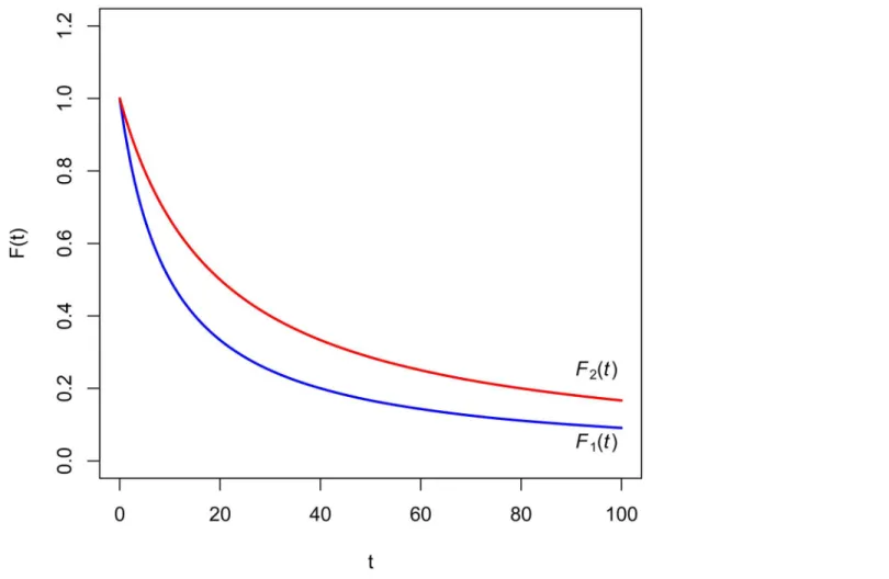
Example 1. LetF1ðtÞ ¼ 1
1þi1tandF2ðtÞ ¼ 1
1þi2tbe two hyperbolic discount functions where
F1(t)<F2(t) (soi1>i2).FF21ððttÞÞ¼ 1þi1t
1þi2tis increasing since d
dt F2
F1
ðtÞ ¼ i1 i2
ð1þi
2tÞ
2>0: ð4Þ
According to Theorem 2,d1ðtÞ ¼ i1
1þi1tmust be greater than
d2ðtÞ ¼ i2
1þi2t. In effect,
d
1ðtÞ d2ðtÞ ¼
i1 i2
ð1þi
1tÞð1þi2tÞ
>0:
Fig 1shows that it is not easy to graphically observe that the ratioF2(t) (shown in red) to
F1(t) (in blue) is increasing.
For this reason we are going to formulate the following
Corollary 1. LetF1(t) andF2(t) be two discount functions such thatF2(t)−F1(t) is
increas-ing. In this case, any of the three equivalent conditions of Theorem 2 is satisfied. For a proof,
seeAppendix.
Fig 1. Hyperbolic discount functions of Example 1.
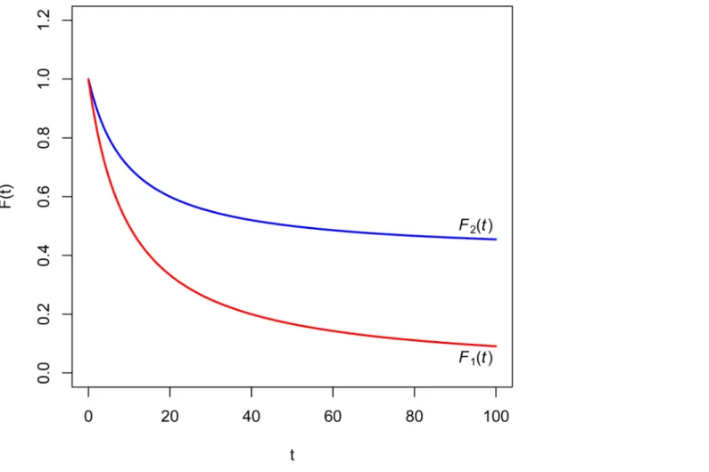
Example 2. LetF1ðtÞ ¼ 1
1þi1tbe a regular hyperbolic discount function of parameteri1and
F2ðtÞ ¼ 1þi2t
1þi1tbe a singular hyperbolic discount function of parametersi1andi2(so necessarilyi1
>i2).Fig 2shows that the differenceF2(t)−F1(t) is increasing.
In effect,
d
dtðF2 F1ÞðtÞ ¼
i2
ð1þi
1tÞ
2 >0: ð5Þ
According to Corollary 1,d 1ðtÞ ¼
i1
1þi1tmust be greater than d
2ðtÞ ¼
i1 1þi1t
i2
1þi2t, which can easily be verified. Then the impatience represented byF1(t) is greater than the impatience
rep-resented byF2(t).Fig 2shows the general situation described by Corollary 1. Finally, the results
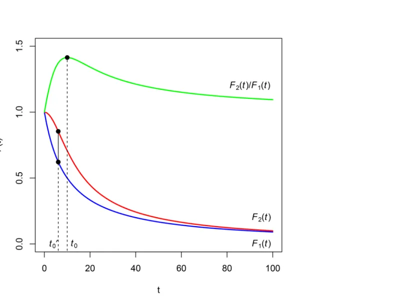
obtained in Theorem 2 and Corollary 1 can be summarized inFig 3. Let us now consider a third situation. Let us suppose that the ratioF2ðtÞ
F1ðtÞreaches a local maxi-mum at instantt0. A possible graphic representation is depicted inFig 4.
By Theorem 2, for intervals [t1,t2] included in [0,t0] (t1,t2<t0), the impatience represented
byF1(t) is greater than the one represented byF2(t). After instantt0, the opposite situation
occurs, that is, the impatience represented byF1(t) is less than that represented byF2(t), but Fig 2. Hyperbolic discount functions of Example 2.
Fig 3. Summary of the results in Theorem 2 and Corollary 1.
doi:10.1371/journal.pone.0149256.g003
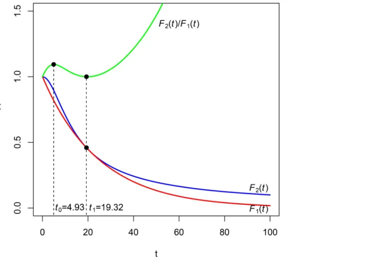
Fig 4. Discount functions of Example 3 and their ratio.
this situation can change becauset0is a local maximum and so there exists the possibility of
another local extreme. For example, ifF2(t) is singular andF1(t) is regular, there will exist a
neighborhood of infinity whereF2ðtÞ
F1ðtÞis increasing.
Example 3. LetF1ðtÞ ¼ 1
1þitbe a hyperbolic discount function of parameteriand
F2ðtÞ ¼ 1 ffiffiffiffiffiffiffiffiffi 1þi2
t2
p ,i>0. Obviously,F1(t)<F2(t) andFF21ððttÞÞreaches a maximum att0¼ 1
i(seeFig 4
wherei= 0.10). In accordance with the previous paragraph,d1ðtÞ ¼ i
1þitis greater thand2ðtÞ ¼
i2
t
1þi2t2in the interval½0; 1
i½¼ ½0;10½, and contrarilyδ2(t) is greater thanδ1(t) in 1
i;þ1½¼10;þ1½.
We can now formulate the following statement.
Theorem 3. LetF1(t) andF2(t) be two discount functions such thatF1(t)<F2(t). IfF2(t)−
F1(t) reaches a local maximum att00, then the factor
F2ðtÞ
F1ðtÞreaches a local maximum at a later instantt0(eventually,t0can be +1).
Example 4. Observe that, for the discount functions of Example 1 withi1= 0.05 andi2=
0.10,F2(t)−F1(t) reaches its local maximum att00 ¼12:610andt0= +1, as predicted by Theo-rem 3.
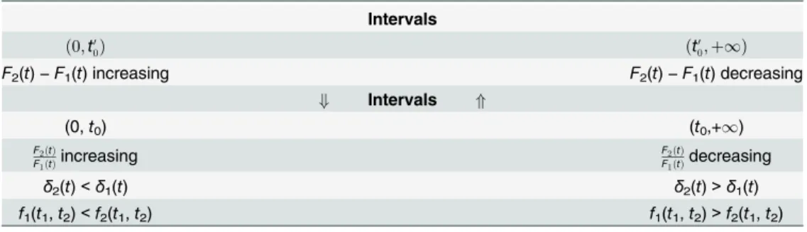
Table 1schematically represents the result obtained in Theorem 3. For the sake of
simplic-ity, we will suppose that bothF2(t)−F1(t) andF
2ðtÞ
F1ðtÞreach a unique local maximum.
Althought0is the instant which separates the intervals whereδ1(t)>δ2(t) andδ1(t)<δ2(t),
there are some intervals [t1,t2], wheret1<t0<t2, such thatf1(t1,t2)<f2(t1,t2). In effect, given
t1<t0, this instantt2must satisfy:
Z t0
t1
½d
1ðxÞ d2ðxÞdx> Z t2
t0
½d
2ðxÞ d1ðxÞdx: ð6Þ
The maximum value oft2must satisfy the following equation:
f1ðt1;t2Þ ¼f2ðt1;t2Þ: ð7Þ
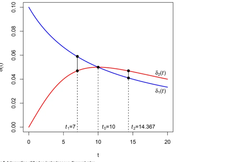
Example 5. LetF1(t) andF2(t) be the discount functions of Example 3. Takingt1= 7, we
have to solve the following equation (seeFig 5):
f1ð7;t2Þ ¼f2ð7;t2Þ;
for which the solution ist2= 14.367.
Finally, this reasoning can be continued by considering the following local extreme ofF2ðtÞ
F1ðtÞ (in this case, a local minimum), and so on.
Table 1. Several implications arising from the relationship between the local maxima ofF2(t)−F1(t)
andF2ðtÞ F1ðtÞ.
Intervals
ð0;t0
0Þ ðt00;þ1Þ
F2(t)−F1(t) increasing F2(t)−F1(t) decreasing
+ Intervals *
(0,t0) (t0,+1)
F2ðtÞ
F1ðtÞincreasing
F2ðtÞ
F1ðtÞdecreasing
δ2(t)<δ1(t) δ2(t)>δ1(t)
f1(t1,t2)<f2(t1,t2) f1(t1,t2)>f2(t1,t2)
Case in which the two functions intersect
For the sake of simplicity, in this Subsection, we will assume that functionsF1(t) andF2(t) only
intersect at an instantt1. In this case, we will distinguish between the following two subcases:
• F1(t) andF2(t) are secant. This situation does not affect the results obtained in Theorems 2
and 3.
• F1(t) andF2(t) are tangent. In this case, F2ðtÞ
F1ðtÞreaches a local extreme at this point and so we can apply Theorem 3. More specifically,F2ðtÞ
F1ðtÞreaches a local minimum att1(seeFig 6) and so, by Theorem 3,δ1(t) is less thanδ2(t) on the left oft1, and contrarilyδ1(t) is greater thanδ2(t) on the right oft1. But observe also that
F2ðtÞ
F1ðtÞreaches a local maximum att0. Thus, the global situation can be summarized inTable 2.
An application to well-known discount functions
In experimental analysis, it is usual to fit the available data from several groups of individuals to discount functions belonging to the same family. It is therefore necessary to compare the impatience represented by two discount functions coming from the same general family.
Fig 5. Intersection of the two instantaneous discount rates.
Comparison of two generalized hyperbolic discount functions
These functions are the well-knownq-exponential discount functions introduced by [41]. Let
F1(t) andF2(t) be two generalized hyperbolic discount functions:
F1ðtÞ ¼
1
ð1þi
1tÞ
s1 ð8Þ
and
F2ðtÞ ¼
1
ð1þi2tÞs2; ð9Þ
Fig 6. Intersection of the two discount functions: case of tangency.
doi:10.1371/journal.pone.0149256.g006
Table 2. Patience / impatience according to different intervals.
Intervals (0,t0) (t0,t1) (t1,+1)
F2ðtÞ
F1ðtÞ % & %
Greater impatience F1(t) F2(t) F1(t)
Greater patience F2(t) F1(t) F2(t)
wherei1>i2. Let us calculate thefirst derivative ofFF12ððttÞÞ: d
dt F2
F1
ðtÞ ¼ð1þi1tÞ
s1 1
ð1þi
2tÞ
s2 1
½s1i1ð1þi2tÞ s2i2ð1þi1tÞ
ð1þi2tÞ2s2 : ð10Þ
We are going to assume thats16¼s2. Otherwise, the comparison betweenF1(t) andF2(t)
would be the same as two hyperbolic discount functions. Making this derivative equal to zero, we obtain:
t0¼
s2i2 s1i1
s1 s2
: ð11Þ
1. Ifs1>s2, thent0<0 and F2ðtÞ
F1ðtÞis increasing in
Rþ. Thus, by Theorem 2(iii),δ1(t)>δ2(t) and
so the impatience represented byF1(t) is greater than the impatience represented byF2(t).
2. Ifs1<s2, we can consider two subcases:
a. s2 < s1i1
i2, in which caset0>0 is a local maximum of
F2ðtÞ
F1ðtÞ. Thus, by Theorem 2, δ
1(t)>
δ
2(t) in (0,t0) andδ1(t)<δ2(t) in (t0,+1) and therefore, according to Theorem 2, the
impatience represented byF1(t) is greater than the impatience represented byF2(t) in the
interval (0,t0) and less in the interval (t0,+1).
b. s2 > s1i1
i2, in which caset0<0 and
F2ðtÞ
F1ðtÞis increasing in
Rþ. Thus, again by Theorem 2,
δ
1(t)>δ2(t) and so the impatience represented byF1(t) is greater than the impatience
represented byF2(t).
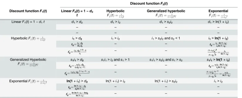
In order to compare the impatience of several well-known discount functions, inTable 3, we have considered the linear, hyperbolic, generalized hyperbolic, and exponential discounting both in the column on the left and on the upper row. Each cell of this table has been divided into three parts. We have represented the cases in which two discount functionsF1(t) andF2(t)
(F1(t)<F2(t)) satisfy the three equivalent conditions of Theorem 2. In this case, the first part
of the cell shows the relationships to be satisfied by the parameters ofF1(t) andF2(t) in order to
satisfy Theorem 2. On the other hand, we have represented in bold those cases whereF1(t) and
F2(t) do not satisfy the conditions of Theorem 2. In theses cases, the first level of the cell
exhib-its the relationships between the parameters ofF1(t) andF2(t) so thatF1(t)<F2(t) in a
neigh-borhood of zero; the second level of the cell includes the maximumt0ofFF21ððttÞÞ; and,finally, the third level contains the maximumt0
0ofF2(t)−F1(t). The relative position of these time instants
was discussed in Theorem 3.
Conclusion
The term impatience was introduced by [2] in 1930 to refer to the preference for advanced tim-ing of future satisfaction. More recently the concept of decreastim-ing impatience has been applied to those situations in which discount rates are decreasing. Usually this property has also been labeled as hyperbolic discounting, although there are other discount functions involving decreasing discount rates. In this paper, we have focused on measuring the degree of impa-tience of discount functions in both intervals and instants.
functions corresponding to two groups of people have been obtained, there arises the problem of comparing the impatience exhibited by each of them.
At first glance, the faster the function decreases, the higher is the degree of impatience. That is, ifF2(t)−F1(t) is increasing, the impatience shown byF1(t) is higher than the impatience
shown byF2(t). But this graphic criterion only represents a condition sufficient to compare
degrees of impatience. Nevertheless, it is convenient to state a necessary and sufficient condi-tion for the impatience ofF1(t) to be higher than the impatience ofF2(t); this condition could
be that the ratioF2(t)/F1(t) is increasing. In Theorem 2, that allows us to compare the
impa-tience associated with two discount functions, we present two conditions equivalent to the for-mer. Unfortunately, it is difficult to observe this property graphically in most cases (unless we consider the difference lnF2(t)−lnF1(t)). In other cases, however, the monotonicity ofF2(t)/
F1(t) changes, necessitating the calculation of its maximum and minimum extreme values
(Theorem 3). In most cases, the comparison of the impatience will be made using two discount functions belonging to the same family. Therefore, the problem of determining the local extremes ofF2(t)/F1(t) can be solved explicitly or, at least, their existence must be
demonstrated.
The main contributions of this paper are Theorems 2 and 3. InTable 3we compare the impatience shown by pairs of discount functions belonging to the most important families of temporal discounting (linear, hyperbolic, generalized hyperbolic and exponential discount functions). Thus, a restriction in red represents a conditionsine qua nonfor a pair of discount functions in order to satisfy Theorem 2. Nevertheless, there are other pairs of discount func-tions not satisfying the condifunc-tions of Theorem 2. In this case, we have deduced (as shown in bold) the expressions oft0and (the equation to be satisfied by)t00which allows us to check the statement in Theorem 3.
These Theorems allow us to compare the impatience shown by two individuals or two groups of people, once their preferences have been fitted to a suitable discount function
Table 3. Cases of application of Theorem 2 or Theorem 3 (in bold), whereF1<F2.
Discount functionF2(t) Discount functionF1(t) LinearF2(t) = 1−d2
t
Hyperbolic F2ðtÞ ¼
1 1þi2t
Generalized hyperbolic F2ðtÞ ¼
1
ð1þi2tÞs2
Exponential F2ðtÞ ¼
1
ð1þi2Þt
LinearF1(t) = 1−d1t d1>d2 d1>i2 d1>s2i2 d1>ln(1 +i2)
– – – –
– – – –
HyperbolicF1ðtÞ ¼ 1
1þi1t i1>d2 i1>i2 i1>s2i2ands2<1 i1>ln(1+i2)
t0¼
i1 d2
2i1d2 – – t0¼
i1 lnð1þi2Þ i1lnð1þi2Þ
t0 0¼
ði1=d2Þ 1=2 1 i1
– – ð1þi1t00Þ
2
ð1þi2Þ t0
0 ¼ i1
lnð1þi2Þ Generalized Hyperbolic
F1ðtÞ ¼ 1
ð1þi1tÞs1
s1i1>d2 s1i1>i2ands1>1 s1i1>s2i2ands1>s2 s1i1>ln(1+i2)
t0¼
s1i1 d2
i1d2ðs1þ1Þ – –
t0¼
s1i1 lnð1þi2Þ
i1lnð1þi2Þ
t0 0¼
ðs1i1=d2Þ 1=ðs1þ1Þ 1 i1
– – ð1þi1t00Þ
s1þ1
ð1þi2Þ t0
0 ¼ s1i1
lnð1þi2Þ ExponentialF1ðtÞ ¼
1
ð1þi1Þt ln(1+i1)>d2 ln(1 +i1)>i2 ln(1 +i1)>s2i2 i1>i2
t0¼ lnð1þi1Þd2
d2lnð1þi1Þ – – –
t0 0¼
ln lnð1þi1Þ lnd2
lnð1þi1Þ – – –
belonging to a well-known family of functions. Finally, this methodology can be applied to two-variable (amount and time) discount functions when some anomalies in intertemporal choice (for example, delay or magnitude effect) are taken into account.
Appendix
Proof of Corollary 1. AsF2(t)−F1(t) is increasing andF1(t) is decreasing, thenF
2ðtÞ F1ðtÞ
F1ðtÞ is increasing. Therefore,F2ðtÞ
F1ðtÞ
1(and consequentlyF2ðtÞ
F1ðtÞ) is increasing which is condition (i) of Theorem 3.
Proof of Theorem 3. AsF2(t)−F1(t) reaches a local maximum att00, then
F0
2ðt00Þ F10ðt00Þ ¼0; ð12Þ
from where
F0 2ðt
0 0Þ ¼F
0 1ðt
0
0Þ: ð13Þ
AsF2(t)>F1(t), andF02ðt00ÞandF10ðt00Þare negative (remember thatF(t) is decreasing), one has
F0
2ðt00ÞF1ðt00Þ>F10ðt00ÞF2ðt00Þ: ð14Þ
HenceF0 2ðt
0
0ÞF1ðt00Þ F 0 1ðt
0
0ÞF2ðt00Þ>0and therefore the factor
F2ðtÞ
F1ðtÞis increasing att 0
0, leading to a local maximum at an instantt0 >t00(eventuallyt0could be +1).
Acknowledgments
This paper has been partially supported by the project“Valoración de proyectos gubernamen-tales a largo plazo: obtención de la tasa social de descuento”, reference: P09-SEJ-05404, Proyec-tos de Excelencia de la Junta de Andalucía and Fondos FEDER. The funders had no role in study design, data collection and analysis, decision to publish, or preparation of the manuscript.
We are very grateful for the comments and suggestions offered by the Editor and three anonymous referees.
Author Contributions
Contributed reagents/materials/analysis tools: SCR MJMT. Wrote the paper: SCR MJMT.
References
1. Koopmans TC (1960) Stationary ordinal utility and impatience.Econometrica28(2): 287–309. doi:10. 2307/1907722
2. Fisher I (1930)The Theory of Interest. Macmillan, London.
3. Böhm-Bawerk EV (1912) Positive Theorie des Kapitals, Dritte Auflage, English Translation in Capital and Interest, 1959, Vol. II, Positive Theory of Capital, Book IV, Section I. South Holland, pp. 257–289. 4. Cheng J, González-Vallejo C (2014) Hyperbolic discounting: value and time processes of substance
abusers and non-clinical individuals in intertemporal choice.PLoS ONE9(11): e111378. doi:10.1371/
journal.pone.0111378PMID:25390941
5. Takahashi T, Oono H, Radford MHB (2007) Empirical estimation of consistency parameter in intertem-poral choice based on Tsallis’statistics.Physica A381: 338–342. doi:10.1016/j.physa.2007.03.038
6. Ainslie G (1975) Specious reward: A behavioral theory of impulsiveness and impulse control. Psycho-logical Bulletin LXXXII: 463–509. doi:10.1037/h0076860
8. Frederick S, Loewenstein G, O’Donoghue T (2002) Time discounting and time preference: a critical review.Journal of Economic Literature40: 351–401. doi:10.1257/jel.40.2.351
9. Cruz Rambaud S, Muñoz Torrecillas MJ (2005) Some considerations on the social discount rate. Envi-ronmental Science and Policy8: 343–355. doi:10.1016/j.envsci.2005.04.003
10. Cruz Rambaud S, Muñoz Torrecillas MJ (2006) Social discount rate: a revision.Anales de Estudios Económicos y Empresariales XVI: 75–98.
11. Thaler R (1981) Some empirical evidence on dynamic inconsistency.Economic Letters8: 201–207.
doi:10.1016/0165-1765(81)90067-7
12. Benzion U, Rapaport A, Yagil J (1989) Discount rates inferred from decisions: An experimental study.
Management Science 35(3): 270–284. doi:10.1287/mnsc.35.3.270
13. Takahashi T, Oono H, Radford MHB (2008) Psychophysics of time perception and intertemporal choice models.Physica A387: 2066–2074. doi:10.1016/j.physa.2007.11.047
14. Takahashi T, Hadzibeganovic T, Cannas SA, Makino T, Fukui H, Kitayama S (2009) Cultural neuroeco-nomics of intertemporal choice.Neuroendocrinology Letters30(2): 185–191. PMID:19675524
15. Kirby K, Marakovic N (1995) Modelling myopic decisions: Evidence for hyperbolic delay-discounting within subjects and amounts.Organizational Behavior and Human Decision Processes 64: 22–30. doi: 10.1006/obhd.1995.1086
16. Myerson J, Green L (1995) Discounting of delayed rewards: Models of individual choice.Journal of the Experimental Analysis of Behavior64: 263–276. doi:10.1901/jeab.1995.64-263PMID:16812772
17. Kirby K (1997) Bidding on the future: Evidence against normative discounting of delayed rewards. Jour-nal of Experimental Psychology: General 126: 54–70. doi:10.1037/0096-3445.126.1.54
18. Takahashi T (2008) A comparison between Tsallis’statistics-based and generalized quasi-hyperbolic discount models in humans.Physica A 387: 551–556. doi:10.1016/j.physa.2007.09.007
19. Myerson J, Green L, Warusawitharana M (2001) Area under the curve as a measure of discounting.
Journal of the Experimental Analysis of Behavior 76(2): 235–243. doi:10.1901/jeab.2001.76-235 PMID:11599641
20. Matta A, Gonçalves FL, Bizarro L (2012) Delay discounting: concepts and measures.Psychology & Neuroscience5(2): 135–146. doi:10.3922/j.psns.2012.2.03
21. Read D (2001) Is time-discounting hyperbolic or subadditive?Journal of Risk and Uncertainty 23(1): 5–32. doi:10.1023/A:1011198414683
22. Prelec D (2004) Decreasing impatience: A criterion for non-stationary time preference and“hyperbolic”
discounting.Scandinavian Journal of Economics106(3): 511–532. doi:10.1111/j.0347-0520.2004. 00375.x
23. Laibson D (1997) Golden eggs and hyperbolic discounting.The Quarterly Journal of Economics112 (2): 443–477. doi:10.1162/003355397555253
24. Halevy Y (2008) Strotz meets Allais: diminishing impatience and the certainty effect.American Eco-nomic Review 98(3): 1145–1162. doi:10.1257/aer.98.3.1145
25. Sayman S, Öncüler A (2009) An investigation of time inconsistency.Management Science55(3): 470–
482. doi:10.1287/mnsc.1080.0942
26. Abdellaoui M, Attema AE, Bleichrodt H (2010) Intertemporal tradeoffs for gains and losses: an experi-mental measurement of discounted utility.The Economic Journal120(545): 845–866. doi:10.1111/j. 1468-0297.2009.02308.x
27. Attema AE, Bleichrodt H, Rohde KI, Wakker PP (2010) Time-tradeoff sequences for analyzing dis-counting and time inconsistency.Management Science56(11), 2015–2030. doi:10.1287/mnsc.1100. 1219
28. Bleichrodt H, Rohde KI, Wakker PP (2009) Non-hyperbolic time inconsistency.Games and Economic Behavior 66(1): 27–38. doi:10.1016/j.geb.2008.05.007
29. Tanaka T, Camerer CF, Nguyen Q (2010) Risk and time preferences: linking experimental and house-hold survey data from Vietnam.American Economic Review 100(1): 557–571. doi:10.1257/aer.100.1. 557
30. Nguyen Q (2011) Does nurture matter: Theory and experimental investigation on the effect of working environment on risk and time preferences.Journal of Risk and Uncertainty43: 245–270. doi:10.1007/ s11166-011-9130-4
31. Espín AM, Brañas-Garza P, Herrmann B, Gamella JF (2012) Patient and impatient punishers of free-riders.Proceedings of the Royal Society B279: 4923–4928. doi:10.1098/rspb.2012.2043PMID: 23075842
33. Caliendo FN, Findley TS (2014) Discount functions and self-control problems.Economic Letters122: 416–419. doi:10.1016/j.econlet.2013.12.035
34. Lu Y, Zhuang X (2014) The impact of gender and working experience on intertemporal choices.Physica A 409: 146–153. doi:10.1016/j.physa.2014.05.015
35. Chen H, Ng S, Rao AR (2005) Cultural differences in consumer impatience.Journal of Marketing Research XLII: 291–301. doi:10.1509/jmkr.2005.42.3.291
36. Hoch SJ, Loewenstein GF (1991) Time-inconsistent preferences and consumer self-control.Journal of Consumer Research17: 492–507. doi:10.1086/208573
37. Seinstra M, Grzymek K, Kalenscher T (2015) Gender-specific differences in the relationship between autobiographical memory and intertemporal choice in older adults.PLoS ONE10(9): e0137061. doi:
10.1371/journal.pone.0137061PMID:26335426
38. Cruz Rambaud S, Muñoz Torrecillas MJ (2013) A generalization of theq-exponential discounting func-tion.Physica A 392(14): 3045–3050. doi:10.1016/j.physa.2013.03.009
39. Musau A (2014) Hyperbolic discount curves: a reply to Ainslie.Theory and Decision76(1): 9–30. doi: 10.1007/s11238-013-9361-8
40. Destefano N, Martinez AS (2011) The additive property of the inconsistency degree in intertemporal decision making through the generalization of psychophysical laws.Physica A 390: 1763–1772. doi: 10.1016/j.physa.2011.01.016
41. Cajueiro DO (2006) A note on the relevance of theq-exponential function in the context of intertemporal choices.Physica A364: 385–388. doi:10.1016/j.physa.2005.08.056
42. Benhabib J, Bisin A, Schotter A (2010) Present-bias, quasi-hyperbolic discounting, and fixed costs.