www.atmos-meas-tech.net/5/1147/2012/ doi:10.5194/amt-5-1147-2012
© Author(s) 2012. CC Attribution 3.0 License.
Measurement
Techniques
Particle sizing calibration with refractive index correction for light
scattering optical particle counters and impacts upon PCASP and
CDP data collected during the Fennec campaign
P. D. Rosenberg1, A. R. Dean2, P. I. Williams3,4, J. R. Dorsey3,4, A. Minikin5, M. A. Pickering6, and A. Petzold5
1School of Earth and Environment, University of Leeds, Leeds, LS2 9JT, UK 2Facility of Airborne Atmospheric Research, Cranfield, MK43 0AL, UK
3School of Earth, Atmospheric and Environmental Sciences, University of Manchester, Manchester, M13 9PL, UK 4National Centre for Atmospheric Science, School of Earth, Atmospheric and Environmental Sciences,
University of Manchester, Manchester, M13 9PL, UK
5Institute of Atmospheric Physics, DLR, Wessling, 82234, Germany 6Met Office, Exeter, EX1 3PB, UK
Correspondence to:P. D. Rosenberg ([email protected])
Received: 19 December 2011 – Published in Atmos. Meas. Tech. Discuss.: 4 January 2012 Revised: 27 April 2012 – Accepted: 27 April 2012 – Published: 21 May 2012
Abstract. Optical particle counters (OPCs) are used regu-larly for atmospheric research, measuring particle scatter-ing cross sections to generate particle size distribution his-tograms. This manuscript presents two methods for cali-brating OPCs with case studies based on a Passive Cavity Aerosol Spectrometer Probe (PCASP) and a Cloud Droplet Probe (CDP), both of which are operated on the Facility for Airborne Atmospheric Measurements BAe-146 research air-craft.
A probability density function based method is provided for modification of the OPC bin boundaries when the scatter-ing properties of measured particles are different to those of the calibration particles due to differences in refractive index or shape. This method provides mean diameters and widths for OPC bins based upon Mie-Lorenz theory or any other particle scattering theory, without the need for smoothing, despite the highly nonlinear and non-monotonic relationship between particle size and scattering cross section. By cali-brating an OPC in terms of its scattering cross section the optical properties correction can be applied with minimal information loss, and performing correction in this manner provides traceable and transparent uncertainty propagation throughout the whole process.
Analysis of multiple calibrations has shown that for the PCASP the bin centres differ by up to 30 % from the
manufacturer’s nominal values and can change by up to ap-proximately 20 % when routine maintenance is performed. The CDP has been found to be less sensitive than the manu-facturer’s specification with differences in sizing of between 1.6±0.8 µm and 4.7±1.8 µm for one flight. Over the course of the Fennec project in the Sahara the variability of calibra-tion was less than the calibracalibra-tion uncertainty in 6 out of 7 calibrations performed.
As would be expected from Mie-Lorenz theory, the im-pact of the refractive index corrections has been found to be largest for absorbing materials and the impact on Saharan dust measurements made as part of the Fennec project has been found to be up to a factor of 3 for the largest particles measured by CDP with diameters of approximately 120 µm. In an example case, using the calibration and refractive in-dex corrections presented in this work allowed Saharan dust measurement from the PCASP, CDP and a Cloud Imaging Probe to agree within the uncertainty of the calibration. The agreement when using only the manufacturer’s specification was poor.
1 Introduction
1.1 Optical particle counters
Light scattering optical particle counters (OPCs) are instru-ments used to measure the concentration and size of air-borne particles. They are used in many fields such as in ground based, aircraft based or balloon based atmospheric research or pollution or clean room monitoring. OPCs func-tion by passing an air sample through a beam of light and detecting the radiation scattered out of the beam by individ-ual suspended particles. OPCs have applications over a wide range of particle sizes from aerosol particles with diameters of 0.06 µm (Cai et al., 2008) to ice and liquid cloud parti-cles with diameters of the order 100 µm (Cotton et al., 2010), although an individual instrument will usually cover a size range of approximately one to two orders of magnitude. A related instrument type known as the optical array probe or imaging probe (Knollenberg, 1970) images the shadow of a particle as it passes through a laser beam and scatters light away. These instruments provide size distributions up to mm sizes. Because of their ability to provide real-time data over many size ranges, OPCs are the de-facto standard for mea-suring particle size distributions, particularly on research air-craft where their fast acquisition speeds are important.
Despite these advantages OPCs do not provide particle diameters explicitly. The amount of light scattered by a particle is defined not only by a particle’s size but also by its shape, refractive index, n, (which may be com-plex in the case of light absorbing materials) and whether or not the particle is homogeneous. These additional vari-ables are particularly important in atmospheric measure-ments where OPCs are often employed to measure many different particle types from spherical homogeneous water-droplets (n= 1.33) to angular volcanic ash particles (nin the range 1.5−1.6 + 0.001i−0.02iMu˜noz et al., 2004; Patter-son, 1981; Patterson et al., 1983).
Designs of OPCs vary enormously; however, there are some features which are common to almost all instruments. Each collects the scattered light over an angular range de-fined by the geometry of the instrument’s optics and focuses this light onto a photo-detecting element. Each particle pass-ing through the beam therefore generates an electrical pulse in a detector circuit. All OPCs measure the height of this pulse and some measure other properties such as pulse width or shape. Some OPCs collate particle events into discrete time and/or pulse height bins (including the Grimm OPC; Heim et al., 2008) while others provide the time and pulse height for every particle at the finest resolution allowed by the electronics (for example the SID2; Cotton et al., 2010).
Assuming an appropriate calibration is performed, the height of each pulse is a direct measurement of a particle’s scattering cross section over the collecting solid angle of the OPC optics. Combining these measurements of particles’ cross sections with knowledge of how cross section varies
with size allows a size distribution to be derived. Performing an effective calibration and scattering properties correction is essential to generate the highest quality data from an OPC. The latter of these is made more difficult because scattering cross section is often not a monotonic function of diameter over much of the size range where OPCs are utilised.
This manuscript describes methods for calibrating OPCs and performing scattering property corrections as well as providing software for the community to use to perform these operations. To overcome the problems associated with utilising a highly nonlinear scattering function, a probabil-ity distribution function (PDF), rather than a single value, is transformed between diameter and scattering cross section or visa-versa. The following basic methodology is applied:
1. Generate a PDF based on the mean diameter (scattering cross section) and it’s uncertainty. Often this will be a Gaussian function representing a normal distribution. 2. Transform this PDF to scattering cross section
(diameter).
3. Generate a mean scattering cross section (diameter) and uncertainty based on the new PDF.
An example of an application of this method is taken from the instrumentation operated by the Facility for Airborne At-mospheric Measurements during the Fennec campaign. 1.2 The Passive Cavity Aerosol Spectrometer Probe and
Cloud Droplet Probe
The Facility for Airborne Atmospheric Measurements (FAAM) operates a number of OPCs on the UK’s BAe-146-301 Atmospheric Research Aircraft. Amongst these are a Passive Cavity Aerosol Spectrometer Probe 100-X (PCASP) and a Cloud Droplet Probe (CDP) which are both mounted externally on the aircraft below the wings.
The PCASP was initially manufactured by Particle Mea-surement Systems but it has since been modified to include the SPP-200 electronics package manufactured by Droplet Measurement Technologies (DMT). The manufacturer spec-ification indicates the instrument measures particles over a diameter range of 0.1 to 3 µm diameter. It is a closed cell instrument meaning that it draws an air sample containing aerosol particles into an optical chamber where it makes its measurements.
is incident upon a crystal oscillator where 0.1 % of the in-cident radiation passes through to a photodetector allowing measurement of the laser intensity and the remaining 99.9 % is reflected back along the reciprocal path. The use of an os-cillator rather than a mirror ensures the direct and reflected beams are not coherent and ensures interference between the beams does not occur. The scattered light is collected by a parabolic mirror which collects light from the direct beam over the angular range 35–120◦and from the reflected beam over the range 60–145◦before a lens focuses it onto a pho-todetector. The signal from the photodetector is processed by three parallel systems: a high, mid and low gain stage. In the manufacturer specifications the three gain stages correspond to particle diameters of 0.1–0.14, 0.14–0.3 and 0.3–3.0 µm. Based on whether the particle registers or saturates on the different gain stages one single value is chosen to represent the pulse height in the range 1–12 288. Based on this pulse height the particle is assigned to one of 30 channels generat-ing a histogram every 0.1, 1 or 10 s.
When operated on an aircraft the PCASP is fitted with a forward facing diffuser inlet and a subsampling inlet which passes a small fraction of sample from the diffuser to the detection optics. The inlet system is discussed in more detail in Sect. 1.3.
The CDP is manufactured by DMT and is specified to de-tect and size cloud droplets with diameters from 2–50 µm. In contrast to the PCASP, which has an internal sampling sys-tem, the CDP is an open path OPC. It consists of two arms, separated by 111.1 mm, which house the detecting compo-nents of the system. A 0.658 µm diode laser is directed out of a sapphire window and between the two arms across an open sample area. In the sample area, particles suspended in an air sample pass through the beam and scatter laser radiation. The unscattered radiation and a subset of scattered radiation pass through a second sapphire window into the detector arm and the intensity of the unscattered beam is measured by a dump spot monitor. Light scattered within the range 4–12◦is passed onto an optical beam splitter where 33 % and 67 % of the light is directed to two detectors known as the Sizer and Qualifier respectively (Lance et al., 2010).
To avoid the need for complex retrieval algorithms, the CDP attempts to screen out all particles which do not pass through a small area of∼0.24 mm2located equidistant from the two arms and known as the instrument’s depth-of-field. This is performed by placing a linear mask over the Quali-fier detector meaning that the ratio of the Sizer to QualiQuali-fier signal is a function of particle position. For accepted parti-cles the analogue Sizer signal is amplified and digitised and the pulse height is measured giving a value in the range 1– 4096. The CDP provides a histogram of pulse heights with 30 bins every second. In addition, it provides the incidence time and pulse height at maximum instrument resolution for the first 256 particles detected per second. This is known as particle-by-particle data. Particle-by-particle data allows par-ticle grouping to be examined and rebinning of parpar-ticles after
logging has taken place. In this way much more information is available and the data is more flexible.
For both instruments it should be noted that identical par-ticles passing through different parts of the sample volume may generate slightly different responses. This smearing of the measured size distribution is due to slight differences in irradiation due to the Gaussian mode lasers used and dis-placement away from the focal point of the optics.
1.3 Further measurement uncertainties
Particle sizing is only one aspect of the function of an OPC. The other is particle concentration measurement. Although this work does not deal directly with this aspect of calibra-tion, it is useful to consider some of the problems which may be encountered with the data presented here. For a closed path instrument with an inlet such as the PCASP, the rep-resentativeness of the concentration measurement is often known as the sampling efficiency and is 1 for perfect sam-pling, less than 1 for undersampling and greater than 1 for oversampling. For an open path instrument such as the CDP the concentration measurement relies upon defining a sample area, also known as the depth of field. The sample area de-fines a cross sectional area of the laser beam through which particles must pass to be counted. Multiplying the sample area by the speed of the airflow through the laser and the measurement time interval provides a sample volume al-lowing a concentration to be measured. Lance et al. (2010) showed that the CDP sample area can be measured using a droplet gun on a micro-positioning system. It should be noted, however, that due to the method used to define the sample area, described in Sect. 1.2, the sample volume may be a function of the scattering properties of the particles mea-sured.
inlet velocity is in the range 0.18–6.0. The PCASP subsam-pling rate has been set to 3.0 cm3s−1on the ground in order
that the flow ratio remains within these limits where possible (note the aircraft speed increases and the subsampling speed decreases with increasing altitude). The data presented here assume an inlet efficiency of 1 for the diffuser and then as-sumes sampling efficiencies based on the mean flow speed at the subsampling inlet and the Belyaev and Levin (1974) relations. It should be noted, however, that flow inside the diffuser is expected to be turbulent as the Reynolds num-ber at the tip may be as high as 60 000 during flight. A 3-dimensional incompressible fluid dynamics model with di-rect numerical simulation of turbulence has confirmed that flow separation occurs in the conical inlet leading to turbu-lent eddies at the subsampler. Further investigation in terms of compressible fluid modelling, inlet comparison and wind tunnel testing will be required to assess the impact of this turbulence on the sampled size distribution. Possible effects include turbulent losses in the diffuser and errors in inlet ef-ficiency of the subsampling inlet.
2 Calibration techniques
2.1 Sample generation and scattering cross section calculation
Because OPCs measure particle scattering cross section di-rectly, calibrations can be performed more easily in terms of this parameter. It is therefore critically important that the cal-ibration particles have well defined scattering cross sections. The two most common types of calibration particles used are polystyrene latex (PSL) spheres and glass beads, both of which are commercially available in samples with very narrow distributions and may be suspended in air to provide a calibration sample. Those used here were calibrated us-ing photon correlation spectroscopy and optical microscopy, traceable via NIST to the Standard Metre. Although these particles have the advantage of a traceable calibration cer-tificate, they are only available in a finite number of dis-crete sizes. This is a particular problem for the PCASP high gain stage which does not span many available sizes of PSL spheres.
Aerosol particles with a broad distribution can also be used for calibration if a well defined subsample can be taken. Here this has been performed by passing the aerosol through a Dif-ferential Mobility Analyser (DMA) (Knutson and Whiteby, 1975). A DMA uses a potential difference to separate par-ticles based on their electrical mobility, which is defined by the stokes equation as
Z= neeC
3π ηDp
, (1)
whereeis the charge on an electron,neis the number of
ad-ditional electrons on the particle,C is the Cunningham slip
correction factorηis the dynamic viscosity of the carrier gas andDpis the particle diameter. The transfer function
(frac-tion of particles transmitted through the DMA) has a narrow triangular shape defined by
T ∝max
0,1−|Z
∗−Z|
1Z
, (2)
whereZ∗ is the mid-point mobility of the distribution and
1Z is the full width at half maximum of the transmission function. We also defineD∗ byZ∗=Z(D∗). Under normal operation1Zis proportional to the ratio of the output flow to the internal sheath flow andZ∗is proportional to the ratio of the potential difference to the internal sheath flow. For use with FAAM’s PCASPs which draw at 3 cm3s−1 values of
1Z/Z∗ of around 5 % are achievable for particle diameters less than 0.5 µm.
A number of aerosol types have been used in this manner. The preferred aerosol is nebulised di(2-ethylhexyl)sebacate (DEHS) with a distribution much wider than the DMA trans-fer function. This material has a well known refractive index and forms stable spherical liquid aerosol particles, making it ideal for use with Mie-Lorenz theory calculations. One dis-advantage is that DEHS is a plasticiser so can attack plastic components. Oleic acid and ammonium sulphate have been tested, but the former reacts with oxygen and the latter does not form perfectly spherical aerosol (Dick et al., 1998; Hud-son et al., 2007).
Mie-Lorenz theory is used to derive the scattering prop-erties of calibration particles as a function of their diameter and refractive index. Mie-Lorenz theory exactly describes the scattering of radiation by homogeneous spheres and here the scattering phase function is derived using the code of Wis-combe (1980). The scattering cross section measured by an OPC is given by the integral of the phase function as
σ= π k2
2π Z
0 π Z
0
S1 θ, kDp, n 2
+S2 θ, kDp, n 2
sin(θ ) woptics(θ, φ)dθdφ (3)
where
– kis the wavenumber of the light used by the OPC, – Dpis the particle diameter,
– nis the particle’s refractive index, – S1 θ, kDp, n
2
+S2 θ, kDp, n 2
is the scattering intensity derived from Mie-Lorenz theory (split into light polarised parallel,S1, and perpendicular,S2, to the
scattering plane),
– φis the direction of the scattered radiation around the incident beam,
– woptics(θ,φ) is a weighting function defined by the
op-tical geometry of the OPC.
The value of woptics(θ, φ) varies from 0 at angles where
no light is collected to 1 where all light is collected. In the PCASP where the beam is incoherently reflected back on it-selfwoptics (θ,φ) may be greater than 1 and in the case of
rotational symmetry around the laser beamwis a function of
θonly. The optical geometry andwoptics (θ) are defined for
the PCASP and CDP in Table 1. For non-calibration particles which do not meet the criteria for Mie-Lorenz theory other more complex scattering theories may be used to define the scattering intensity for Eq. (3). The impact upon misalign-ment of the optics of the CDP and PCASP is discussed fur-ther in Sect. 4.3. It should be noted that for OPCs where the particles are measured within the laser cavity of an external-cavity laser (so-called active external-cavity OPCs) Eq. (3) should be replaced with one of the sensitivity functions given by Pin-nick et al. (2000). Also OPCs which do not collect light sym-metrically around the laser may need to take account of the laser polarisation.
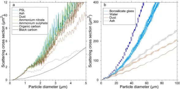
Figure 1 shows scattering cross sections as a function of diameter for PSL spheres, DEHS and glass beads for the PCASP and CDP, as well as other real world materials (as-suming Mie-Lorenz theory). It is clear that in general the curve is highly nonlinear and that above diameters of around 1 µm it is not monotonically increasing. Given the complex-ity of the Mie-Lorenz curve, it is non-trivial to convert from particle diameter to scattering cross section where an uncer-tainty must be propagated. The usual method of propagating uncertainty by multiplying by a function’s gradient cannot in general be used, because the curve cannot be assumed linear over the range of the uncertainty. Instead we convert from di-ameter to cross section by integrating over a PDF. Here we choose a normal distribution with standard deviation equal to the uncertainty in particle diameter. In this case the equiva-lent particle scattering cross section and its uncertainty for a particle diameterDp±1Dpis
σp= R∞
0 σ Dp
G DpDp, 1Dp
dDp R∞
0 G DpDp, 1Dp
dDp
(4)
and
1σp= v u u t
R∞ 0 σp Dp
−σp 2
G DpDp, 1DpdDp R∞
0 G DpDp, 1Dp
dDp
(5)
where1 represents uncertainty andG(Dp,Dp,1Dp)is a
Gaussian function ofDpwith mean/modeDpand standard
deviation 1Dp. As described in Sect. 1 a Gaussian
func-tion is chosen to represent normally distributed uncertain-ties. Again, becauseσp(Dp)is a highly nonlinear function,
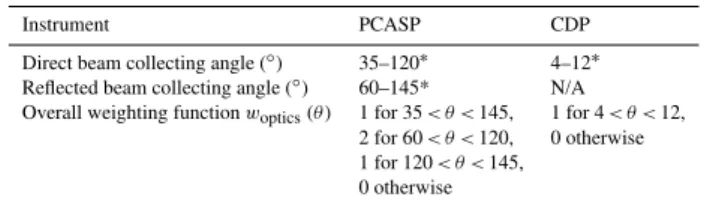
Table 1.Collecting angles of the PCASP and CDP optics and
asso-ciated values ofwoptics(θ ).
Instrument PCASP CDP
Direct beam collecting angle (◦) 35–120∗ 4–12∗
Reflected beam collecting angle (◦) 60–145* N/A
Overall weighting functionwoptics(θ ) 1 for 35< θ <145, 1 for 4< θ <12, 2 for 60< θ <120, 0 otherwise 1 for 120< θ <145,
0 otherwise
∗Nominal values based on manufacturer specifications. Instrument-to-instrument variation is discussed in Sect. 4.3.
σp will not in general be equal toσp(Dp). Converting the
mode diameter of our calibration particles into cross section in this way ensures that the OPC is calibrated in terms of the property it directly measures. These calculations can be performed for any particles where scattering cross section is known as a function of diameter and are not dependent upon using Mie-Lorenz theory.
2.2 Calibration methods
2.2.1 Calibration introduction
Two different methods have been developed when calibrat-ing the probes. A discrete method was used with the finite number of PSL spheres and glass beads available as well as using a DMA. A scanning method was also used with a DMA which allowed many closely spaced distributions to be generated sequentially. These two methods are applicable to different calibration scenarios described in detail below. 2.2.2 PCASP and CDP calibration setup
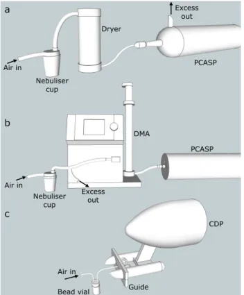
When calibrating the FAAM OPCs the instruments and sam-ple generation equipment were set up as shown in Fig. 2. When calibrating the CDP a flow of air is forced through a vial of glass beads. These are suspended in the sample and directed through a guide to the sample area of the laser. Be-cause the calibration particles are larger than a few microme-tres, contamination from ambient air does not usually pose a problem. The flow rate from the compressed gas supply is manually regulated in to provide a few hundred particles per second as measured by the CDP. This concentration is used to avoid coincidence which can cause problems above
∼500 s−1(Lance et al., 2010) and yet provide a useful
parti-cle distribution in a short time period. The concentration of smaller bead sizes in the sample tends to be more difficult to control which can result in high concentrations and coinci-dence of particles in the laser beam. Clumping of small par-ticles, especially in moist conditions or when the air supply is cold, can also be a problem. Because of these problems, only particles with diameters larger than 15 µm were used here.
Fig. 1.Mie-Lorenz curves showing scattering cross sections for a variety of materials as measured by a PCASP(a)and a CDP(b). Refractive indices are taken from Bond and Bergstrom (2006), Dinar et al. (2006, 2008), Highwood et al. (2011), Mu˜noz et al. (2004), Patterson (1981), Patterson et al. (1983), Toon et al. (1976), Wagner et al. (2012), Volten et al. (2001), Cook et al. (2007) and Weast (1966). The two curves for Saharan dust and volcanic ash approximately bound a range of refractive indices found in the literature. For borosilicate glass the two curves represent the two different refractive indices given by the manufacturer for different samples of calibration beads.
The sample is drawn through the DMA using the PCASP’s pump. This requires the nosecone to be removed and the DMA output to be connected to the PCASP subsampler using push on flexible tubing. When using nebulised PSL spheres the sample line may be connected to the subsampler as when using a DMA or the sample may be directed into the PCASP conical inlet in which case the positive pressure from the neb-uliser pump floods the subsampler with the PSL loaded air. All tubing used is electrically conductive and as short as pos-sible to minimise losses. Again a counting rate of a few hun-dred particles per second is used.
The nebuliser cup used in this work was an Allied Health-care Aeromist model SA-BF61403. These cups can be oper-ated using a pump or a compressed air supply using a needle valve to regulate flow.
2.2.3 Discrete method
Because an OPC measures scattering cross section directly it is possible to define a simple function which relates parti-cle scattering cross section to pulse height. This function will be defined by the OPC detector and electronic systems. The PCASP and CDP use only linear amplifiers therefore we ex-pect that pulse height will be a linear function of scattering cross section.
When calibrating an OPC in this manner there are two re-quirements.
1. The scattering cross sections of the calibration particles must be known.
2. The pulse heights measured by the OPC are known or, in cases where particles are binned into a histogram by the OPC, the bin boundaries must be known in terms of pulse height.
Simply knowing the manufacturer’s estimate of bin boundary in terms of diameter is not sufficient unless the equivalent pulse height can be derived from these values.
For the PSL spheres and glass beads used in PCASP and CDP calibrations, the scattering cross section along with an uncertainty were derived from Eqs. (3)–(5). This satisfies condition (1) above. The PCASP and CDP are both provided with a list of bin boundaries in terms of pulse height known as a threshold table. This table is modifiable to allow re-programming of the instruments and satisfies condition (2) above making these OPCs suitable for use with this method. To perform the calibration using PSL spheres and glass beads the PCASP and CDP are set up as shown in Fig. 2 and as described in Sect. 2.2.2. For calibrating the high gain stage of the PCASP only two useful sizes of PSL sphere were available to the authors’ knowledge. Therefore, another source of calibration particles was needed. In this case we made use of the DMA with nebulised DEHS aerosol. Using the DMA as set up in Fig. 2, values ofD∗in the range 0.1– 0.5 µm were set in steps of 0.003–0.01 µm. Using the DMA in this way ensured the generation of sufficient data points to effectively calibrate the high gain stage of the PCASP.
a
b
c
Air in
CDP
Bead vial Air in
Excess out
PCASP Dryer
Nebuliser cup
Excess out Air in
DMA
PCASP
Nebuliser cup
Guide
Fig. 2. Calibration setup for the PCASP and CDP OPCs. The
PCASP is either calibrated using nebulised PSL spheres(a)or a DMA with nebulised DEHS oil aerosol(b)and the CDP is cali-brated with dry dispersed glass beads(c). When used with the DMA the PCASP conical inlet is removed and the sample line is con-nected directly to the subsampler. During calibration of the CDP a guide attaches to the instrument arms to direct the sample into the sample area.
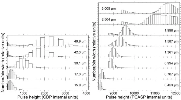
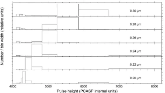
in the calibration. To reduce this uncertainty the PCASP is reprogrammed to zoom in on a particular size range of in-terest. In this way the uncertainties in particle diameter are comparable to the uncertainties in pulse height measured by the PCASP. It was not necessary to reprogram the CDP as its 30 bins over its single gain stage contribute an uncertainty of similar magnitude to the calibration beads. Examples of the measured particle distributions as a function of pulse height are shown in Fig. 3 for PCASP and CDP.
To generate a calibration equation for the OPCs, the mode particle scattering cross section and associated uncertainty for each of the calibration particle samples is derived from Eqs. (3)–(5). These are then plotted against the equivalent mode pulse heights measured by the instruments as seen in the particle distributions in Fig. 3. The mode of the pulse heights is preferred to the mean because it is affected less by particle coincidence and contamination of the sample and can be used even when a part of the size distribution is outside the range of the OPC. In particular when using PSL spheres from solution, dried surfactant can generate
significant contamination which can affect the distribution mean but not the mode.
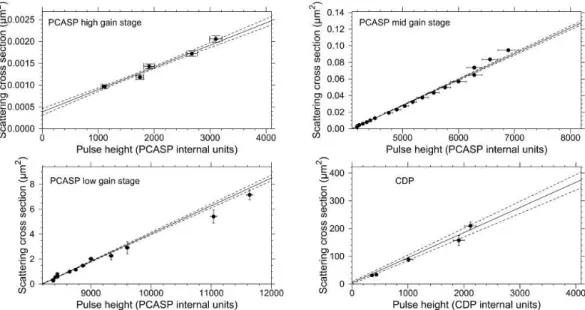
Figure 4 shows example calibration data for the CDP and PCASP along with 1-sigma uncertainties. Each data point represents a particular size of calibration particle. The un-certainties in scattering cross sections in Fig. 4 are derived from Eq. (5) and the uncertainties in pulse height are half the width of the modal bin in the measured particle distribu-tion. The straight line fits to the data take into account uncer-tainties on both axes (Cameron Reed, 1989, 1992) to give a sensitivity,s, and offsetV0along with uncertainties. We can
then simply derive a particle’s scattering cross section with uncertainty for any pulse height,Vp, as
σp=V0+sVp, (6)
1σp2=1V02+1s2Vp2+2Vpcov(V0, s), (7)
where cov(V0,s) is the covariance of the two variables.
The PCASP provides a single size distribution spanning all three gain stages. At the boundaries the gain stages over-lap and in the overover-lap region particles are counted by only one gain stage. This causes a narrowing of one channel in each gain stage which should be trivial to account for from the calibration. Despite applying this information to the bin boundaries, artefacts in the size distribution always exist at these overlap points. These are discussed in more detail in Sect. 3.
2.2.4 Scanning method
For some OPCs it is not possible to easily record the pulse heights associated with each particle or with the bin bound-aries. This may be because the pulse height measurements and binning are performed using analogue electronics which are not easy to characterise or it may be because the manu-facturer does not make the information available to the user. In this case the OPC can be calibrated using a tuneable par-ticle source where the parpar-ticle size distribution may be ad-justed in an almost continuous manner. This technique has been used to calibrate the FAAM PCASP using a DMA al-though the processing is more complex compared to the dis-crete method. Although this description is based upon using a DMA with a PCASP, any other OPC and tunable particle source could be used, such as an impactor or a droplet gen-erator in the super-micrometre range.
Fig. 3.Particle response distributions generated during calibration of the CDP (left) and PCASP (right). The horizontal axis shows the instrument response to the particles and the vertical axis shows the number of particles measured in each response bin. The labels indicate the mode diameter of the particles used to generate each distribution. For the PCASP only a subset of the used PSL sphere particle distributions are shown and the high resolution is achieved by reprogramming the instrument to zoom in on the area of interest. The broad distribution for the 2.504 µm spheres may be caused by the close proximity to a spike in the Mie-Lorenze curve. The CDP particle distributions were generated using glass beads.
use this parameter to determine its diameter equivalent. For an OPC withN bins measuring mi particles in the ith bin
andMparticles in total we can defineF as
F =
N P
i=n+1 mi
M . (8)
For an OPC which does not bin particles into a histogram we can consider one bin to be the diameter/pulse height resolu-tion of the instrument. The particle size distriburesolu-tion of the calibration aerosol,Pp(Dp)can be related toF by
F =
R∞ DbnPp Dp
dDp R∞
0 Pp Dp
dDp
(9) whereDbn is the diameter of the boundary between binsn
andn+ 1. It should be noted that Eq. (9) is based on the as-sumption that all of the particle size distribution falls within the range of the OPC and it is critical that this is verified dur-ing the calibration. As already discussed the particle scatter-ing cross section for DEHS is monotonically increasscatter-ing over the range where this technique is used, allowing us to use di-ameter in Eq. (9). For larger didi-ametersDshould be replaced byσ.
Because the DMA transfer function contains multiple peaks for multiply charged particles, as represented byne
in Eq. (1), it is required that an OPC calibrated in this way has the resolution to identify the peaks representingne>1
and that these peaks are discarded from the analysis. Alter-natively these particles can be physically removed from the sample, for example by using an impactor or another size se-lective removal method.
When dealing with only a single peak it is possible to rigorously defineP(Dp)for Eq. (9) by applying the DMA
transfer function from Eqs. (1) and (2) to the DEHS size dis-tribution generated by the nebuliser (which can be assumed to be linear over a narrow size range). However, for the distri-butions used in this work it was found thatF can be approxi-mated by an integrated Gaussian (sigmoid) to within 1 % and doing so impacts the result by only∼0.1 %. Specifically
F ≈1
2
1+erf
D∗
−Dbn
√
2W2
, (10)
where the function erf is the error function andWis a mea-sure of the distribution width. This function is much simpler than a more rigorous definition ofF and also is likely to bet-ter represent random deviations from other uncertainties in the system. It is useful to note that due to the symmetry of Eq. (10)F= 0.5 whenD∗=Dbn, i.e. when the mode of the DMA output is at a bin boundary, 50 % of particles fall either side of the boundary.
Fig. 4.Particle scattering cross section as a function of pulse height for an example calibration of the PCASP and CDP. The points represent the modes of size distributions generated from calibration particles with scattering cross sections defined by Eq. (4). The uncertainties in the horizontal direction are defined as half the OPC resolution and those in the vertical direction are defined by Eq. (5). The solid line shows the best fit straight line when uncertainties on both axes are utilised dashed line shows the standard error of the best fit.
uncertainty in this estimate can be derived by combining the standard error output from the data fitting routine with the uncertainty in the DMA using the usual uncertainty combi-nation functions.
A series of particle distributions from a DMA calibration are shown in Fig. 5. The resolution is much poorer than in Fig. 3 because the bin boundaries for normal use are main-tained for this calibration rather than zooming in on a region of interest. The secondary charged peak for theD∗= 0.2 µm spectrum is just visible, however it has been smeared out due to the resolution of the PCASP in this region of the distribu-tion. The number of particles counted by the PCASP in the doubly charged peak was more than 50 % of the number in the singly charged peak, so it is clear this peak would have a large impact upon calculations ofF if not discarded.
The values ofF derived from all the size distributions col-lected as part of this calibration are shown in Fig. 6. The best fit curves are derived from Eq. (10). Each of the curves provides the upper boundary of one bin and in all cases the standard error in this boundary estimate is less than 0.3 % giving an uncertainty in bin width of between 1 and 10 %. In addition the uncertainty for the DMA is∼1 %. This is of a similar order to the discrete method.
3 PCASP gain stage boundaries
As described earlier the PCASP uses three separate gain stages to maximise its range. If a pulse saturates the first gain stage it is passed to the second. If it saturates this gain stage it is passed to the third and if it saturates the third gain stage
it is registered as oversized. Where the first gain stage over-laps the second gain stage it reduces the width of the first bin of the second gain stage. This is because some particles that would be measured by the second gain stage do not saturate the first gain stage so are instead counted in the top bin of the first gain stage. A similar process occurs where the second and third gain stage overlaps. After performing the calibra-tion detailed in Sect. 2.2.3 independently for each gain stage, the limiting boundaries of the gain stages must be compared. Where an overlap occurs the bottom of one gain stage must be set to the top of the previous gain stage.
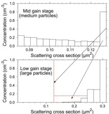
Unfortunately, despite this correction, size distributions from the PCASP tend to show concentrations which are too high in the top bin of each gain stage and too low in the first bin of the second and third gain stage. It is suggested here that particles are not correctly registering as saturated so are getting stuck in the top bin of a gain stage. To investigate this problem the PCASP was reprogrammed to zoom in on the overlap region between the mid and low gain stages (medium and large particles). The particle distributions as a function of scattering cross section for the two gain stages are shown in Fig. 7. A number of unexpected features are evident here:
1. The concentration in the low gain stage remains zero for some distance beyond the overlap point.
2. The last bin in the mid gain stage has enhanced concentrations.
Fig. 5.Particle size distributions measured during a scanning cali-bration of a PCASP using a DMA. Each bin is normalised by divid-ing by its width. The resolution here is not as good as in Fig. 3, as the bin boundaries used here are those for normal use so no zoom-ing in is applied. Only data collected by the mid gain stage is shown. The labels indicate the mode diameter,D∗, set on the DMA when generating each distribution. Peaks can be seen from particles with double charges which pass through the DMA forD∗≤0.26 µm at pulse heights above approximately 5800. The doubly charged peak at a pulse height of 6300 withD∗= 0.20 contains more than one third of the total particles in this distribution. These extra peaks must be removed from the analysis to avoid biasing the calibration results.
4. The concentration in the last bin of the low gain stage is significantly enhanced.
In addition, the concentration of oversized particles is only 0.028 cm−3 which is much lower than expected given the concentration in the top bin of 2.47 cm−3, and the bin be-fore this of 0.30 cm−3. This plot seems consistent with our hypothesis that particles are getting stuck at the top of a gain stage and are not effectively moving to the next gain stage or being classified as oversized. At the very least, some un-documented process is affecting the distribution at the gain stage boundaries. Unfortunately, the mechanism causing this problem is not known, however, an effective workaround is to merge the bins either side of each gain stage boundary and discard the final bin of the PCASP.
4 Refractive index correction
4.1 The perfect, zero uncertainty case
As has already been stated the scattering cross section of a particle is a function of its refractive index n, diameter
Dp, shape and structure. For OPCs calibrated using the
dis-crete method above, applying this refractive index depen-dence is implicit in the conversion from scattering cross sec-tion to diameter. For an OPC calibrated in terms of diameter, such as when using a DMA to calibrate the sub-micrometre range of a PCASP as described in Sect. 2.2.4, then the bin
Fig. 6.An example scanning calibration result using a DMA with
a PCASP. Each curve represents one bin boundary and is an un-weighted fit to the data points. They show how the fraction of parti-cles bigger than a boundary,F, increase as the DMA mode diame-ter,D∗, increases. The value ofD∗at which a best fit curves crosses 0.5 defines the boundary’s equivalent diameter. Multiply charged particles from the DMA were screened out during the data analysis. The uncertainty inD∗is∼1 %.
boundaries must be first converted to scattering cross section using Eqs. (3)–(5).
For a spherical particle Mie-Lorenz theory can be used to perform the conversion from scattering cross section to diam-eter. Although Fig. 1 shows that this is relatively straightfor-ward for sub-micrometre particles, it is clear that for super-micrometre particles where the Mie-Lorenz curves are not monotonic there are a number of challenges to overcome. For example:
– Multiple diameters may correspond to a single scatter-ing cross section.
– The gradient at each solution will differ making uncer-tainties more difficult to interpret.
– The uncertainty may be large enough that the function significantly deviates from linear within a few error bars of the cross section of interest. This means that the un-certainty cannot be simply transformed using the func-tion’s gradient.
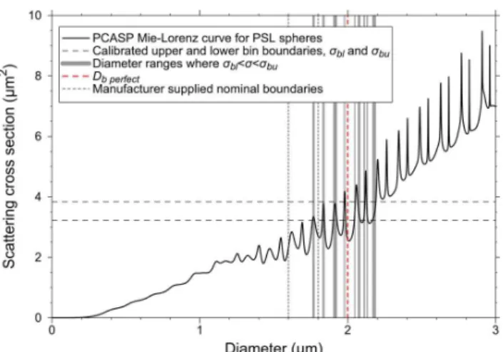
The first point above is highlighted particularly if we wish to derive the edges of an OPC bin in terms of diameter, and then subtract one from the other to derive a bin width. It is very likely that the multiple solutions derived from the two boundaries will overlap in diameter space and the overlap may span most of the range of the solutions. Such a case is shown in Fig. 8 where the boundaries of a PCASP bin calibrated before the Fennec campaign are shown along with the Mie-Lorenz curve for PSL spheres.
Fig. 7.The two plots show details at a PCASP gain stage boundary created by reprogramming a PCASP to zoom in on this area of inter-est. The red vertical bar shows the maximum extent of the overlap between the two gain stages, below which we expect to see no par-ticles. The horizontal red bar shows the concentration which would be measured if the excess in the top channel of the mid gain stage were redistributed above the overlap point of the low gain stage. Note that the top bin of the low gain stage goes off the scale to a concentration of 2.47 cm−3.
of the same composition as the particles measured in the real world. Others have smoothed theoretical curves or widened the bins of the OPC to generate a monotonically increasing function or reduce the effect of this ambiguity upon each bin (Johnson and Osborne, 2011; Liu et al., 1974). These meth-ods either suffer from a lack of generality, being only ap-plicable to particles of specified refractive indices or ranges of refractive indices, or requires a subjective assessment of the amount of smoothing required. Baumgardner (2012) sug-gested a method that defined an instrument kernel matrix. This kernel would transform the real world particle size dis-tribution into the measured disdis-tribution, based on the parti-cle scattering properties and instrument calibration. The real world size distribution could be recovered by finding the in-verse of the kernel matrix. This method has been examined and tested as part of this work, however, some limitations were found regarding numerical stability and error propa-gation so this method has been discounted in favour of the method presented below.
Here a rigorous method is presented which is general to any scattering function of arbitrary complexity without the need for smoothing. By examining Fig. 8 it is clear that in terms of diameter, each OPC bin has multiple boundaries.
There are, however, other properties of a bin which provide enough information to derive a size distribution, can be de-scribed in terms of diameter, are easily visualised and may be rigorously defined. For normalisation purposes it is essential that we define the bin’s width,Wb, which can be performed
by summing the widths of all the sub-ranges highlighted by grey vertical bars in Fig. 8. By averaging the centres of the sub-ranges weighted by their widths we can also define a bin mean,Db, in terms of diameter. If there is a requirement to
define the bins in terms of another quantity such as parti-cle area, volume or log of diameter, then the horizontal axis of Fig. 8 may be transformed appropriately. The bin mean and bin width defined in this way provide equivalent infor-mation to bin boundaries and so can be used as a direct re-placement when calculating size distributions, mass/volume loadings and other derived quantities. The bin centre and bin width as described above are defined as
Db perfect(σbu, σbl)= R∞
0 P (D, σbu, σbl) DdD R∞
0 P (D, σbu, σbl)dD
(11)
Wb perfect(σbu, σbl)= ∞ Z
0
P (D, σbu, σbl)dD (12)
Where P(D, σbu, σbl) is the probability that a particle
with diameter D falls within a bin with upper and lower boundaries at σbu and σbl, i.e. P(D, σbu, σbl)= 1 when σbl< σ(D)< σbuand 0 otherwise. The subscript perfect
in-dicates that this is the perfect case with no uncertainties. It should be noted that values ofDb perfectfor adjacent bins may
be closer or more distant than may be indicated by the values ofWb perfect. This is an effect of the interleaving of bins seen
in Fig. 8 and a fundamental property of OPCs. Over a large diameter range any perceived overlaps or gaps will cancel. 4.2 Propagation of calibration uncertainties
If, as will always be the case in the real world, there are un-certainties associated with the bin boundaries then these must be propagated into our estimates ofDbandWb. Two factors
have a specific impact here. Because of the highly nonlinear Mie-Lorenz curve, the expectation forDbandWb may not
be equal toDb perfectandWb perfect. Also the uncertainties in σblandσbuwill not be independent if they are derived from
the same straight line fit, meaning that the usual uncertainty propagation formulae may not be applicable.
To accommodate these issues consideration is given to what happens if we vary a bins upper and lower boundaries,
σbu and σbl. This causes different values of Db perfect and Wb perfect to be generated and this variation defines a
sensi-tivity of these parameters to the bin boundaries. By assign-ing a PDF to the variation in the bin boundaries a PDF of the resulting values ofDb perfectandWb perfectis produced which
Fig. 8.Example showing the range of sizes of PSL spheres which would fall within a single bin of a PCASP. The grey shading covers all diameter ranges where the Mie-Lorenz curve falls between the horizontal dashed lines derived from calibration. The mean diame-ter of the shaded regions,Wb perfect, is shown as a vertical red line. The vertical dotted lines show the manufacturer’s boundaries for the same bin.
If our best estimate of the bin’s upper and lower boundary and their uncertainty areσbu,σbl,1σbuand1σblthen we can
use these to define the PDF,w(σl,σu). The integrals which
gives us the resultsDb,Wband their associated uncertainties
are then
Db= R∞
0 R∞
0 Db perfect(σbu, σbl) w (σbu, σbl)dσbudσbl R∞
0 R∞
0 w (σbu, σbl)dσbudσbl
, (13)
1D2b= R∞
0
R∞
0 Db perfect(σbu, σbl)−D
2
w (σbu, σbl)dσbudσbl
R∞
0
R∞
0 w (σbu, σbl)dσbudσbl
, (14)
Wb= R∞
0 R∞
0 Wb perfect(σbu, σbl) w (σbu, σbl)dσbudσbl R∞
0 R∞
0 w (σbu, σbl)dσbudσbl
, (15)
1Wb2= R∞
0
R∞
0 Wb perfect(σbu, σbl)−W2w (σbu, σbl)dσbudσbl
R∞
0
R∞
0 w (σbu, σbl)dσbudσbl
. (16) Some careful consideration should go into the definition of
w(σbl,σbu)as this function will not be the same in all cases.
Whereσblandσbuare independent we can definew(σbl,σbu)
as the product of two normal distributions.
w (σbl, σbu)=G (σbl, σbl1σbl) G (σbu, σbu1σbu) (17)
This would be the case if the scanning calibration method has been used and the random uncertainties from the curve fitting dominate over any offset in particle diameter that may exist. This is not the case whenσblandσbuare derived from
the same straight line fit. Instead,w(σbl,σbu)can be defined
with reference to the gradient and intercept of the straight line fit, their uncertainties and their covariance. Hence, we replacew(σbl,σbu)withw(s,V0)and integrate over dsand
dV0instead of σbu andσblin Eqs. (13)–(17). The function w(s,V0)is defined by
w (s, V0)=Gbivariate(s, s, 1s, V0, V0, 1V0, Rs,V0), (18) whereGbivariateis a bivariate Gaussian distribution andRs,V0 is the correlation coefficient betweensandV0.
The CDP is calibrated using the discrete method with a straight line fit so utilises Eq. (18). The PCASP’s three separate gain stages are again calibrated using the discrete method so again Eq. (18) is used, however, at the point where the gain stages meet one bin has its lower boundary defined by one straight line fit and its upper boundary by another fit. This bin therefore has two independent boundaries so Eq. (17) is used here.
This method allows the refractive index correction to be determined directly from a Mie-Lorenz or another scattering curve, without the need for smoothing. In addition, software tools have been developed and made freely available ensur-ing that performensur-ing these corrections becomes trivial. 4.3 Uncertainties in scattering properties and curves
The uncertainty propagation presented thus far has assumed that the scattering curve which is generated using Eq. (3) is a perfect representation of the response of an OPC to a par-ticle of a particular size. In reality the weighting function
woptics(θ,φ) will have an uncertainty associated with it as
will the refractive index of the particles being measured. For particles which deviate from perfect spheres, the assumption of Mie-Lorenz scattering or use of a different scattering func-tion may also introduce uncertainty. As will be detailed in Sect. 5, the impact of refractive index and particle shape has not been studied here, however, the variation in probe geom-etry and its input into the instrument uncertainty has been examined. For both the PCASP and the CDP the sampling is symmetric about the laser axis, hence, two possible devia-tions from nominal are considered:
1. A simple change in the limits presented in Table 1. Such a change could represent a deviation of an aperture’s di-mensions from nominal or a movement of the sample volume along the axis of the laser from its expected po-sition. For the PCASP only the 35◦and 145◦limits are varied as these are most sensitive to the position of the laser/sample intersection point. For the CDP the total angular range is maintained at 8◦by altering both limits by the same amount. This is referred to as an along axis deviation.
145◦ limits of the PCASP are considered. These esti-mates were made using a four point integration around the laser axis. The four points were perpendicular to the deviation (where change from nominal is approximated as zero) and parallel to the deviation (where change from nominal is maximised). We refer to this as a lat-eral deviation.
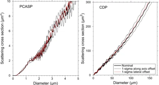
Measurements of the position of the laser beam of the PCASP during alignment have shown that a maximum lateral deviation of 1 mm can be expected. A similar uncertainty is expected for the along axis deviation. Both these misalign-ments give changes in the 35◦and 145◦collecting angle lim-its of approximately 10◦. For the CDP Lance et al. (2010) found that a lateral deviation of 1.4 mm gave the best fit to calibration data, this equates to a deviation of∼2◦. Consid-eration of an along axis deviation was not presented in that work. Baumgardner (2012) reported that the manufacturers of the CDP have begun testing the responses of this instru-ment to small particles in order to estimate its collecting an-gles. They have found maximum deviation of the lower col-lection angle limit of 0.7◦. A higher variation was found for the upper collection angle limit, but this has less impact upon the instrument sensitivity. As the majority of these numbers are maximum offsets of a relatively small population of mea-surements, they have been assumed here to be 2-sigma esti-mate. Therefore the 1-sigma uncertainty in collecting angles of a typical PCASP and CDP used in this work have been assumed to be 5◦and 0.4◦, respectively, for along axis devi-ations and 5◦and 1◦, respectively, for lateral deviations.
For the PCASP we found almost no variation in response to desert dust for lateral deviation of 1-sigma. 1-sigma along axis deviation did, however, lead to a significant change in response. For the CDP, lateral deviation did induce some changes in response, but these were smaller than for along axis deviations. Mie-Lorenz curves for these cases are pre-sented in Fig. 9. Because in both cases the along axis uncer-tainties dominate we shall consider only these here. It should be noted, however, that these conclusions are valid only for the refractive index in question. For the CDP the variation in signal due to misalignment was found to be smaller for glass bead calibration particles and water (not presented here) than for dust.
These uncertainties can be accounted for by calculating
σ(Dp) for different scattering angle limits and assigning
each of these curves a weight. Here seven curves have been used varying between±3-sigma and the weights have been assigned based on a normal distribution. Recalling that each estimate ofDbandWbare derived from a PDF, each curve
can be considered to generate a PDF of possible solutions. These PDFs can be multiplied by the weights and summed to give a final PDF which can be integrated to find its mean and standard deviation. Finding the PDF’s mean reduces to sim-ply calculating the weighted mean of the multiple solutions
giving the bin midpoint and weights including uncertainty in cross section as
Db1σ = P
i Dbiwi
P
i wi
(19)
Wb1σ = P
i Wbiwi
P
i wi
. (20)
The uncertainty can be found by integration giving
1D2b1σ= P
i
wiR0∞ D−Db1σG D, Dbi, 1DbidD
P
i wi
(21)
1Wb21σ= P
i
wiR0∞(W−Wb1σ)G (W, Wbi, 1Wbi)dW
P
i wi
. (22)
Subscriptirepresents the multiple solutions,wiis the weight
of each solution and subscript1σindicates that uncertainties in scattering cross section have been included. In this way contributions from the scatter in the multiple solutions and from the uncertainties derived from Eqs. (14) and (16) are included in the final uncertainty estimate.
Although here the curves forσ(Dp)have been varied to
represent uncertainty in instrument optical parameters this method is equally valid for representing uncertainty in par-ticle refractive index or another scattering property. In ad-dition, multiple properties could be varied and appropriate weights assigned and the resulting solutions can all be passed into Eqs. (19)–(22) together if required.
5 Results and impact upon the Fennec dataset
Fig. 9. Mie-Lorenz curves for the PCASP and CPD showing the impact of misalignment of the optics for desert dust. The thick black line shows the scattering cross section measured by the instruments using the nominal manufacturer’s specification. The thin red and black lines show the impact of moving the sample/laser intersect point or sample volume along the laser axis or laterally in a direction perpendicular to the laser axis. The 1-sigma offsets are estimates of the variation from nominal for a typical instrument and are based observed offsets of FAAM’s PCASP after realignments, measurements of a number of CDPs by the manufacturer (Baumgardner, 2012) and measurements by Lance et al. (2010).
As Fig. 8 shows, the actual ranges from a PCASP bin can vary significantly from the values provided by the man-ufacturer. In the calibration performed before Fennec the bin centres were found to be systematically higher than those reported by the manufacturer by an average of 13 % and a maximum of 33 %. This was based on the use of a refractive index for PSL spheres as used in the manufacturer’s specifi-cation. Monitoring the calibration results over approximately 1 yr has shown that after routine maintenance, such as clean-ing and alignclean-ing the optics, the calibration may change by up to 20 %. This result is consistent with the 35◦and 145◦limits of the PCASP collection optics, varying by up to 10◦as dis-cussed in Sect. 4.3. The drift over time is typically much less than this and calibrations performed before and after projects which have lasted a month or more show less than 5 % drift. During Fennec the CDP was calibrated seven times and these have been examined to check the stability of the instru-ment over this time period. One calibration resulted in a sig-nificantly larger sensitivity than the others, but it is thought that this calibration was affected by high winds so has been discounted from the analysis. For the remaining six calibra-tions all values ofsandV0were found to agree within their
uncertainties. Examining the first calibration performed dur-ing Fennec again revealed that bin centres were systemati-cally higher than those reported by the manufacturer. In this case the refractive index of water was used, again in ac-cordance with the manufacturer’s specification. The largest difference was found near the lowest end of the size range with the centre of bin 2 differing by 4.7±1.8 µm from the
expected value of 3.5 µm. A minimum offset of 1.6±0.8 µm was found.
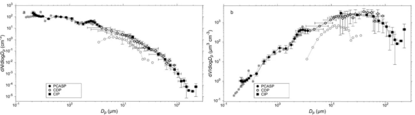
Size distributions from one time period during the Fennec project are shown here. This case consists of 150 s of data beginning at 10:10:30 UTC and collected at 800 m above the desert surface (1080 m GPS altitude). This was a measure-ment period with particularly high dust loadings. There is some uncertainty in the refractive index and shape of the dust measured and here it has been assumed that the dust particles are spheres with a refractive index of 1.53 + 0.003i which lies in the range measured by Wagner et al. (2012). Labo-ratory measurements have shown that Mie-Lorenz calcula-tions can have some success in modelling the scattering prop-erties of non-spherical particles. In the forward scattering angles, as measured by the CDP, laboratory measurements of bulk desert dust samples, including Saharan dust, agreed with Mie-Lorenz calculations within 20 % when surface area equivalent diameters were used (Volten et al., 2001; Kahnert et al., 2007). The scattering cross sections of∼0.2 µm salt particles as measured by a PCASP were modelled by Mie-Lorenz theory to within experimental uncertainties when mean crystal length equivalent diameter was used (Lui et al., 1992). It is beyond the scope of this paper to evaluate the many scattering theories which have been applied to non-spherical particles, and hence based on the successes above Mie-Lorenz theory has been used.
Fig. 10.Size distribution of desert dust aerosol measured by the PCASP, CDP and CIP during a run at 800 m above the desert surface. For the PCASP and CDP, the distributions derived using the manufacturer’s specification are in grey and the calibrated and refractive index corrected data are in black. The number,N, and volumeV, are shown as a function of particle diameterDp. Error bars which extend to negative numbers on the log scale have been omitted for clarity.
boundaries. During Fennec the CDP had been set with bin 1 much wider than usual allowing the CDP to be sensi-tive to smaller particles. To subsequently improve the res-olution in this region, the CDP’s particle-by-particle feature has been used to rebin the particles from bin 1 into 5 sepa-rate bins. These are the first 5 CDP bins plotted in the cali-brated data in Fig. 10. No equivalent manufacturer’s specifi-cations are available for these rebinned points so CDP point 1 of the manufacturer’s specification distribution is equiva-lent to point 6 of the calibrated, refractive index corrected distribution.
The distributions using the manufacturer’s specification are discontinuous at the boundary between the two instru-ments around 4 µm, and the PCASP data shows a zigzag in the distribution at 0.3 µm (the boundary between the mid and low gain stages) and a peak in number concentration in the last channel as described in Sect. 3. A similar zigzag is usu-ally seen at the high to mid gain boundary at around 0.14 µm. The gain stage boundary corrections described in Sect. 3 have been applied to the calibrated data set.
The calibrated data can be seen to extend to much larger diameters than that processed using the manufacturer’s spec-ification. This is mostly due to the impact of the different refractive index of the measured dust compared to the refrac-tive indices of PSL spheres and water droplets referenced by the manufacturer. The two instruments are in excellent agree-ment where they meet and any discontinuity is much less than the 1-sigma error bars plotted. Some bumps seen in the PCASP distribution have been accentuated by the calibration and refractive index correction presented here. It could be the case that these are real modes or there is the potential that this is an artefact caused by imperfect knowledge of the particle scattering properties. The error bars are a significant fraction of the mode height so the statistical significance of this peak is not clear. A strong advantage of the methods used here is the derivation of error bars for this plot which are traceable and transparent which allow consideration of the statistical significance of such modes.
In addition to the OPC data, Fig. 10 also shows data from the Cloud Imaging Probe (CIP), which was part of the Cloud, Aerosol and Precipitation Spectrometer (Baumgardner et al., 2001) operated during Fennec. The CIP is an imaging probe as initially described by Knollenberg (1970). The instrument directs a laser at a linear array of photodetectors and when a particle travels through the laser, perpendicular to the array, its shadow is imaged line-by-line. Utilisation of data from this instrument provides a comparison with a completely dif-ferent particle sizing technique. The CIP, CDP and PCASP all agree within the uncertainties providing high confidence that the calibration and refractive index correction methods presented here work well and that the uncertainty propaga-tion is effective.
It is of note that despite data being available for particles as large as 200 µm, Fig. 10 shows that the measurements do not cover the large diameters of the volume distribution as well as the small diameters. It is clear that the volume distribution of desert dust can have contributions from particles larger than have previously been measured on an airborne platform.
6 Software tools
As part of developing the methods for the calibration and refractive index correction three software tools, known as MieConScat, PCASP Calibrator and CStoDConverter have been created. These are available to the community as open source projects free for academic use via the Source-Forge repository (http://sourceforge.net). MieConScat gener-ates particle scattering cross sections using Mie-Lorenz the-ory as described in Eq. (3). Text files can be saved giving particle cross section as a function of particle diameter, an-gular range, particle refractive index and wavelength of the incident light. This output can be used by the two subsequent programs.
distributions are generated, manual review and quality con-trol can be performed and the modes of these distributions are used to generate a sensitivity curve for the three gain stages. This tool can use the output from MieConScat for de-riving cross sections or text files can be generated by another method if Mie-Lorenz theory is not appropriate.
CStoDConverter accepts bin boundaries defined in terms of scattering cross sections and generates bin centres and widths in terms of diameter using the method described in Sect. 4. The conversion implicitly performs refractive index correction by using either the output from MieConScat or a similarly formatted text file generated any other way if Mie-Lorenz theory is not appropriate.
7 Conclusions
Two methods have been described here for calibrating opti-cal particle counters (OPCs) which are based on the principle that an OPC measures an electrical pulse height which is re-lated to a particle’s scattering cross section. The two methods are referred to as the discrete and scanning methods. The dis-crete method utilises particle samples available only at a fi-nite number of different diameters, and fits a sensitivity curve between the pulse height measured by the OPC and the scat-tering cross section of the particles. This method requires the user to have some access to the pulse heights measured by the OPC, and has been used to calibrate a Passive Cavity Aerosol Spectrometer Probe (PCASP) and a Cloud Droplet Probe (CDP). The scanning method can be used when OPC pulse heights are not accessible but requires a sample size distribution which can be adjusted in a continuous manner. The PCASP has been calibrated using this method with a differential mobility analyser (DMA). The DMA provides a continuously adjustable sample of DEHS oil aerosol with mode diameter,D∗, up to 0.5 µm. A sigmoid-type function was fitted giving the fraction of particles larger than a given bin boundary,F, as a function ofD∗. The diameter equiva-lent of the bin boundary is given by the value ofD∗whereF
is equal to 0.5.
A transparent and mathematically well defined method for refractive index correction has been provided. This method allows OPC bin centres and widths to be defined using Mie-Lorenz theory or any other scattering theory. It can be ap-plied even when particle scattering cross section as a function of diameter is highly nonlinear and non monotonic, thereby avoiding the need for smoothing. It also provides effective methods of uncertainty propagation.
Calibrating a PCASP and a CDP using these methods has shown that particle sizing by the PCASP differs up to 30 % and by the CDP by approximately 1.6±0.8 to 4.7±1.8 µm from the manufacturer’s specification and that a step change in the PCASP calibration of up to 20 % can occur when rou-tine maintenance is carried out. The drift in the calibration over a project with duration∼1 month is better than 5 % for
the PCASP and less than the calibration uncertainty for the CDP. The calibration has revealed inconsistencies with the expected behaviour where different gain stages of the PCASP meet. These can be overcome by discarding the upper bin of the PCASP and merging adjacent bins either side of a gain stage boundary. Desert dust size distributions collected by the PCASP and CDP as part of the Fennec project show entirely consistent results with each other and with a Cloud Imag-ing Probe when calibration and refractive index corrections are performed as described in this work. Data processed us-ing the manufacturer’s specification gives size distributions which are not consistent. In addition, a general shift towards larger particle diameters (up to a factor of 3 at diameters of approximately 100 µm) is observed when the calibration and refractive index corrections described here are applied.
In order that the community can implement similar cali-bration procedures and refractive index corrections with min-imal effort, a series of software tools with source code have been made available for community use. These are applica-ble not only to the PCASP and CDP but to other OPC models as well.
Some further work is required to continue to improve the data quality from the PCASP and CDP. The sampling effi-ciency of the PCASP should be derived for aircraft speeds, which may require a combination of inlet comparisons, wind tunnel tests and modelling. Methods for experimentally de-termining the optical geometry of both these instruments should be developed to attempt to reduce any artefacts in the measured size distributions.
Acknowledgements. The Fennec project was funded by the Natural Environment Research Council (NERC). This work was additionally supported by the DIAMET project also funded NERC. Airborne data was obtained using the BAe-146-301 Atmospheric Research Aircraft [ARA] flown by Directflight Ltd and managed by the Facility for Airborne Atmospheric Measurements [FAAM], which is a joint entity of NERC and the Met Office. We would like to acknowledge all the staff at Droplet Measurement Technologies who regularly work with the staff at FAAM to ensure that the instruments discussed here are in the best possible condition, as well as Jonathan Crosier and Ian Crawford for their work with the CIP data, and Claire Ryder and Steven Abel for testing the methods and software presented in this manuscript. Finally, we would like to thank Darrel Baumgardener and the two other anonymous referees whose input has doubtless improved the quality of the manuscript.
Edited by: M. Wendisch
References