Regional disaster impact analysis: comparing Input-Output and Computable General Equilibrium models

(1)

NHESSD

3, 7053–7088, 2015

Regional disaster impact analysis

E. E. Koks et al.

Title Page

Abstract Introduction

Conclusions References

Tables Figures

◭ ◮

Back Close

Full Screen / Esc

Printer-friendly Version Interactive Discussion

Discussion

P

a

per

|

Discussion

P

a

per

|

Discussion

P

a

per

|

Discussion

P

a

per

|

Nat. Hazards Earth Syst. Sci. Discuss., 3, 7053–7088, 2015 www.nat-hazards-earth-syst-sci-discuss.net/3/7053/2015/ doi:10.5194/nhessd-3-7053-2015

This discussion paper is/has been under review for the journal Natural Hazards and Earth System Sciences (NHESS). Please refer to the corresponding final paper in NHESS if available.

Regional disaster impact analysis:

comparing Input-Output and Computable

General Equilibrium models

E. E. Koks1, L. Carrera2, O. Jonkeren3, J. C. J. H. Aerts1, T. G. Husby1,4, M. Thissen3, G. Standardi2, and J. Mysiak2

1

Institute for Environmental Studies (IVM), VU University Amsterdam, Amsterdam, the Netherlands

2

Fondazione Eni Enrico Mattei (FEEM), Venice, Italy

3

PBL Netherlands Environmental Assessment Agency, The Hague, the Netherlands

4

TNO, Delft, the Netherlands

Received: 30 September 2015 – Accepted: 10 November 2015 – Published: 24 November 2015

Correspondence to: E. E. Koks (elco.koks@vu.nl)

Published by Copernicus Publications on behalf of the European Geosciences Union.

(2)

NHESSD

3, 7053–7088, 2015

E. E. Koks et al.

Title Page

Tables Figures

◭ ◮

Back Close

Full Screen / Esc

Discussion

P

a

per

|

Discussion

P

a

per

|

Discussion

P

a

per

|

Discussion

P

a

per

Abstract

A large variety of models has been developed to assess the economic losses of disas-ters, of which the most common ones are Input-Output (IO) and Computable General Equilibrium (CGE) models. In addition, an increasing numbers of scholars has devel-oped hybrid approaches; one that combines both or either of them in combination with 5

non-economic methods. While both IO and CGE models are widely used, they are mainly compared on theoretical grounds. Few studies have compared disaster impacts of diﬀ_{erent model types in a systematic way and for the same geographical area,}

us-ing similar input data. Such a comparison is valuable from both a scientific and policy perspective as the magnitude and the spatial distribution of the estimated losses are 10

likely to vary with the chosen modelling approach (IO, CGE, or hybrid). Hence, regional disaster impact loss estimates resulting from a range of models facilitates better deci-sions and policy making. Therefore, in this study we analyze one specific case study, using three regional models: two hybrid IO models and a regionally calibrated version of a global CGE model. The case study concerns two flood scenarios in the Po-river 15

basin in Italy. Modelling results indicate that the diﬀ_{erence in estimated total (national)}

economic losses and the regional distribution of those losses may vary by up to a fac-tor of seven between the three models, depending on the type of recovery path. Total economic impact, comprising all Italian regions, is negative in all models though.

1 Introduction

20

In the last few decades we observe an increasing amount of economic activity in areas prone to natural disasters in the world, in combination with a rising frequency of ex-treme weather and climate events (IPCC, 2012). As a result, the need for high quality disaster impact models is becoming more urgent. Therefore, not just a large amount, but also a great variety of models has been developed for this purpose. While the most 25

(3)

Com-NHESSD

3, 7053–7088, 2015

E. E. Koks et al.

Title Page

Tables Figures

◭ ◮

Back Close

Full Screen / Esc

Discussion

P

a

per

|

Discussion

P

a

per

|

Discussion

P

a

per

|

Discussion

P

a

per

|

putable General Equilibrium (CGE) models, an increasing number of scholars employ hybrid models, combining the two or either of them with diﬀ_{erent (partly non-economic)}

models (Baghersad and Zobel, 2015; Carrera et al., 2015; Koks et al., 2015). This wide variety of models, however, leads to an important question: how should (diﬀ_{erences in)}

the outcomes of the models be interpreted? 5

While both IO and CGE models are used widely, a comparison between their results often remains rather theoretical (e.g. Rose, 1995, 2004; Okuyama and Santos, 2014) or between diﬀ_{erent case studies (e.g. Okuyama, 2010). Few studies exist in which}

both model types are empirically compared in a systematic way for the same case study and geographical area using identical input data (Hu et al., 2014; West, 1995). 10

Such a comparison is highly valuable from both a scientific and policy perspective as the magnitude and spatial distribution of losses may vary. It is possible that investments in risk reduction appear justified on account of a certain model while disproportionally high according to another model. Alternatively, regions not directly aﬀ_{ected but with}

trade relations with a region hit by a natural disaster may display either gains or losses 15

depending on the choice of the model. Regional disaster impact loss estimates result-ing from a range of model outcomes facilitates better decisions and policy makresult-ing.

In this study we analyze the disaster impact for two flood scenarios in the North-ern Italy (Po River Basin District) area using three models: two hybrid IO models and a regional CGE model for Italy. We first discuss the main model characteristics. After 20

that, we apply the models and compare their results. The two hybrid input-output mod-els used in this study are the commonly used Adaptive Regional Input-Output (ARIO) model developed by Hallegatte (2008), and the MultiRegional Impact Assessment (MRIA) model, developed by Koks and Thissen (2014). The CGE model used in this study is a regionalized version of the CGE model developed by Standardi et al. (2014), 25

which has been applied already in Carrera et al. (2015) for a disaster impact analy-sis. In the remainder of the paper the CGE model will be indicated as IEES (Italian Economic Equilibrium System).

(4)

NHESSD

3, 7053–7088, 2015

E. E. Koks et al.

Title Page

Tables Figures

◭ ◮

Back Close

Full Screen / Esc

Discussion

P

a

per

|

Discussion

P

a

per

|

Discussion

P

a

per

|

Discussion

P

a

per

The paper proceeds as follows. In Sect. 2, we discuss the valuation of economic losses and provide an overview on important modeling aspects involved in disaster impact analysis. This section includes both a theoretical comparison between IO and CGE models and a brief overview of the proven model extensions from the literature. This is followed by an explanation of the used models in this comparison exercise 5

and the used data in Sect. 3. In Sect. 4, we present the study area and in Sect. 5 the results of the comparison will be presented and in Sect. 6 they will be discussed. Finally, Sect. 7 concludes with providing some lessons learned and recommendations for practitioners and policy makers in the field of disaster risk modelling.

2 Current practices in disaster impact analysis

10

Before turning to the methodological aspects, it is essential to understand what is con-ceived as disaster and what types of economic losses are referred in this paper. Disas-ter is not equivalent to natural hazard. According to the revised UNISDR Disas-terminology (UNISDR, 2015), hazards are ‘potentially damaging physical events, phenomena or human activities’ that may cause harm, while disasters are serious disruptions be-15

yond the capacity to coping with the suﬀ_{ered harm. More generally, hazard strikes turn}

into a disaster when communities or societies at large are unable to cope, with own resources, with the manifold economic, physical, social, cultural and environmental im-pacts of hazard strikes. Consequently, hazard research focuses often on modelling physical disrupting events only, while disaster research should always comprise soci-20

etal impacts (often in economic terms) as well as the post-disaster reconstruction and the recovery (Okuyama and Chang, 2004).

2.1 Economic loss valuation

In the recent scientific literature on the economic impacts of disasters, there is often a diﬀ_{erentiation between two types of losses: stock and flow losses (Bockarjova, 2007;}

(5)

NHESSD

3, 7053–7088, 2015

E. E. Koks et al.

Title Page

Tables Figures

◭ ◮

Back Close

Full Screen / Esc

Discussion

P

a

per

|

Discussion

P

a

per

|

Discussion

P

a

per

|

Discussion

P

a

per

|

Okuyama and Santos, 2014; Okuyama, 2003; Rose, 2004). Stock losses can be de-fined as damage that arises from destruction of physical and human capital. Tangible stock losses result from asset damage. Flow or production losses can also be used to address damage on productive capital but more frequently flow losses refer to busi-ness interruption and interference in up- and downstream supply chains (Okuyama and 5

Santos, 2014). In contrast to asset losses, flow losses are often the main focus in the economic literature (see e.g. Hallegatte, 2008; Rose and Wei, 2013; Okuyama, 2014). In the rest of the paper, we will refer to flow losses as output losses. These flow losses are commonly subdivided into short-term (up to five years) and long-term (more than five years) eﬀ_{ects (Cavallo and Noy, 2009).}

10

2.2 IO models vs. CGE models: a theoretical comparison

The most frequently used models in the current disaster impact modelling literature are econometric models, social accounting matrix (SAM) models, IO models and CGE models. Econometric models, based on time-series data, have the advantage of being statistically rigorous and have predictive skills, but can only provide estimates of the 15

total (aggregated) impacts (Rose, 2004). Reduced-form estimates of disaster losses from econometric models reveal little about the potentially substantial ripple-eﬀ_{ects of}

a disaster. SAM models on the other hand, which are very similar to IO models, are capable of measuring the diﬀ_{erent orders of indirect e}ﬀ_{ects throughout the system of}

diﬀ_{erent economic agents (Okuyama and Sahin, 2009; Seung, 2014). SAM models}

20

are, however, rarely applied. One of the main reasons might be that SAM’s are not often constructed by national bureaus of statistics, and if they are constructed they are specifically build for CGE models since they are a prerequisite to CGE models.

IO and CGE are the most commonly applied models to assess the economic im-pacts of disasters. In general, a standard IO model can be described as a static linear 25

model which presents the economy through sets of interrelationships between sectors themselves (the producers) and others (the consumers). A neoclassical CGE model is a system of equations in which perfect competition is assumed in products ‘market

(6)

NHESSD

3, 7053–7088, 2015

E. E. Koks et al.

Title Page

Tables Figures

◭ ◮

Back Close

Full Screen / Esc

Discussion

P

a

per

|

Discussion

P

a

per

|

Discussion

P

a

per

|

Discussion

P

a

per

and factor endowments are fully employed. In each region the representative firm imizes profits under a technological constraint and a representative household max-imizes consumption utility under a budget constraint. The macroeconomic closure is neoclassical and this means that the investment is saving driven. A fixed proportion of the household income is allocated to saving, the global bank collects all the world sav-5

ings and uses them for investments which are perfectly mobile at the global level. Trade balance is endogenously determined. The two models are characterized by a number of diﬀ_{erences. The most important di}ﬀ_{erence between IO models and CGE model is the}

partial economic analysis in IO modelling vs. the general equilibrium analysis in CGE modelling. The general equilibrium approach stands for a closed economic system 10

where not only all products that are produced are used elsewhere, but where also all in-come earned is spend on diﬀ_{erent products (possibly via savings on investments). The}

general equilibrium approach describes therefore the complete economy, accounting for all monetary and non-monetary flows. Partial economic analysis such as IO analysis does not link income to expenditure. They are therefore demand-driven models where 15

higher/lower income earned in a region does not lead to more/less products demanded. Moreover, how the system is closed with respect to the financial markets will to a large extent aﬀ_{ect the type and the distribution of the e}ﬀ_{ects (Taylor and Lysy, 1979; Thissen}

and Lensink, 2001). The largest diﬀ_{erence in the closures are demand-determined}

investment-driven CGE models and supply-determined savings-driven CGE models. 20

We will chose here for a CGE model with a neoclassical savings-driven closure since these type of models are the most diﬀ_{erent from the demand-determined IO models.}

As shown in Table 1, we can define a number of other diﬀ_{erences. First, in an IO}

context the costs of substitutions of commodities (which would change technical co-eﬃ_{cients) are costly and unlikely to be made in the short run (Crowther and Haimes,}

25

2005). For an IO approach to be suitable, a disturbance must be long enough to take eﬀ_{ect but also short enough to avoid excessive substitutions. Short-term e}ﬀ_{ects are}

(7)

NHESSD

3, 7053–7088, 2015

E. E. Koks et al.

Title Page

Tables Figures

◭ ◮

Back Close

Full Screen / Esc

Discussion

P

a

per

|

Discussion

P

a

per

|

Discussion

P

a

per

|

Discussion

P

a

per

|

(Thissen, 2004). Second, IO models are often praised for their simplicity and abil-ity to explicitly reflect the economic interdependencies between sectors and regions for deriving higher-order eﬀ_{ects. CGE models, on the other hand, are more complex}

because they include supply-side eﬀ_{ects and allow for more flexibility due to their}

non-linearity regarding inter-sectorial deliveries, substitution eﬀ_{ects and relative price}

5

changes. Third, as a result of the diﬀ_{erent economic mechanisms, the outcomes often}

diﬀ_{er as well. Due to their linearity and incapability to include e}ﬀ_{ects of resilience}

mea-sures (the price mechanism being an important one), IO models are often considered to overestimate the impacts of a disaster. CGE models, on the contrary, are said to underestimate the impacts because of possible extreme price and quantity changes 10

which result from the included elasticities (Rose, 2004). Fourth, substitution of prod-ucts and production factors between regions and producers are not possible in the standard Leontief based IO model while they are likely to occur in a post-disaster sit-uation. Substitution eﬀ_{ects are taken into account in CGE models where the Leontief}

production function used in the IO models by more flexible functional forms such as 15

Cobb–Douglas, or Constant Elasticity of Substition (CES) based functions. Last, IO models generally do not handle supply constraints but model a supply perturbation by means of an artificial demand reduction. CGE models include reduced supply capaci-ties.

To overcome some of the shortcomings of traditional IO models for disaster risk mod-20

elling, several extensions1 have been developed. For instance, Okuyama et al. (2004)

1

In this paper we diﬀ_{erentiate between extended models and hybrid models. An extended} model is defined as either a traditional IO or CGE model which is extended by a specific module to make it more compatible for the proposed research question. Examples are Santos and Haimes (2004) and Rose and Liao (2005). A hybrid model, on the other hand, is defined as an IO or CGE model which is combined with a diﬀ_{erent (non)-economic model. More specifically,} the IO or CGE model is altered in such a way, that only the most important theoretical rules are kept. The model is adjusted in such a way that it cannot be directly described anymore as an IO or a CGE model as such. Examples are Hallegatte (2008), Carrera et al. (2015) and Koks et al. (2015).

(8)

NHESSD

3, 7053–7088, 2015

E. E. Koks et al.

Title Page

Tables Figures

◭ ◮

Back Close

Full Screen / Esc

Discussion

P

a

per

|

Discussion

P

a

per

|

Discussion

P

a

per

|

Discussion

P

a

per

have explicitly included a time horizon by applying the Sequential Industry Model (SIM), which allows for an assessment of the eﬀ_{ect of a disaster dynamically over time.}

An-other model which has been widely used and applied is the Inoperability Input-Output Model (IIM), developed by Santos and Haimes (2004). This model has also been dynamically extended (the DIIM) to include the time aspect Besides adding a time 5

and resilience dimension, IO models have also been extended in space by applying an interregional model instead of the traditional single-region model (see e.g. Cho et al., 2001; Kim et al., 2002; Okuyama et al., 2004; Crowther and Haimes, 2010; MacKenzie et al., 2012). CGE models have been extended and further developed as well, to make them more suitable for the modelling of disasters. For instance, Rose 10

and Liao (2005) have developed a CGE model, where they recalibrated the production function to account for resilience. In spatial CGE models (e.g. Tsuchiya et al., 2007; Shibusawa et al., 2009) the distance between agents in the economy is explicitly incor-porated as a dimension (i.e. interregional modelling).

2.3 Taking the best of both worlds: hybrid models

15

Hybrid models are either a combination of IO and CGE models (i.e. CGE modelling characteristics) or a combination of either of them with another type of model. Koks et al. (2015) have coupled an IO model with a biophysical model to improve the ac-curacy of modelled economic disruption. Carrera et al. (2015) and Ciscar et al. (2014) have coupled a CGE model with a biophysical model. Husby et al. (2015) combine 20

a Spatial CGE model with an agent-based model of opinion dynamics to analyze macroeconomic eﬀ_{ects from an increase in public concern. As can be interpreted from}

In den Bäumen et al. (2015), for instance, traditional multiregional input-output model-ing may result in overestimation of the eﬀ_{ects in the non-a}ﬀ_{ected regions when not}

con-sidering the substitution possibilities between the imports from diﬀ_{erent regions.}

CGE-25

models, on the contrary, have the potential to underestimate the impacts because of possible extreme substitution eﬀ_{ects and price changes (Rose, 2004) especially in the}

(9)

NHESSD

3, 7053–7088, 2015

E. E. Koks et al.

Title Page

Tables Figures

◭ ◮

Back Close

Full Screen / Esc

Discussion

P

a

per

|

Discussion

P

a

per

|

Discussion

P

a

per

|

Discussion

P

a

per

|

might provide the “best of both worlds”. One of the most well-known hybrid IO model with CGE characteristics is the ARIO model, developed by Hallegatte (2008, 2014). ARIO allows for production bottlenecks and rationing (see also Sect. 3.1). Another ex-ample is the TransNIEMO model, which is a coupling between a multiregional IO model and a transportation network model, which assesses economic consequences arising 5

from disruption of highway network (Park et al., 2011). Finally, more research is being done recently in combining IO modelling with linear programming (LP) (see e.g. Rose et al., 1997; Baghersad and Zobel, 2015; Koks and Thissen, 2014).

3 Models and data

Figure 1 shows the methodological approach undertaken in this study. A flood damage 10

assessment is performed on two flood scenarios along the Po river in Northern Italy. The economic disruption, as a result of each of the floods, will be prepared for each model. Stock losses are then translated into flow losses by mean of the three economic models. Outputs are systematically compared to investigate the key characteristics of the models and their significance. Table 2 provides a preliminary analysis of the 15

key characteristics of models, based on the descriptions as provided in the following sections.

3.1 From stock losses to flow losses

We assess production losses by converting the asset losses (stock) to a reduction in value-added (flow). This conversion is done using a Cobb–Douglas (CD) production 20

function, while assuming constant returns to scale. A standard CD production function, as shown in Eq. (1), translates the production inputs, capital (K_j) and labor (L_j) into the amount of output (Y_j) per sectorj, whereb_j is the total factor productivity per sector andα andβare output elasticities (Cobb and Douglas, 1928).

Y_j =_b jK

α j L

β

j (1)

25

(10)

NHESSD

3, 7053–7088, 2015

E. E. Koks et al.

Title Page

Tables Figures

◭ ◮

Back Close

Full Screen / Esc

Discussion

P

a

per

|

Discussion

P

a

per

|

Discussion

P

a

per

|

Discussion

P

a

per

To avoid a possible underestimation of the production losses, the assumption of con-stant returns to scale is essential (see Koks et al., 2015 for an extensive explanation). In standard input-output modelling, capital and labor belong to the value-added part of the model. As such, the CD function translates the direct damages into a reduction in value-added (Y_j in Eq. 1). Consequently, the change in value added (∆_Y_j_{) can be}

5

translated into losses in total production (X_j). The economic disruption per sector (σ_j) is defined as:

σ_t_,_j = Yt,j

X_t_,_j

∆_Y t,j

Y_t_,_j (2)

The economic disruption per sector (the right part of Eq. 2) can be seen as the part of the sector in the aﬀ_{ected region that is not possible to “operate” (Santos and Haimes,}

10

2004). This disruption, or shock, will be referred to as the sector inoperability vec-tor. The following step is to assess by how much the natural disaster aﬀ_{ects the total}

production. This can be done by multiplying the total production with the sector inop-erability vector, as shown by Eq. (3), with X being the vector of the total production andσ as the sector inoperability vector. In Eq. (3),X_tis defined as the new production 15

level in time periodt. In the first run, the new time period is considered to be the new post-disaster economic situation. From the post-disaster situation, we can continue to simulate the short-run recovery period (Koks and Thissen, 2014).

X_t0(1−σt,j)=Xt,j (3)

3.2 The ARIO model

20

(11)

NHESSD

3, 7053–7088, 2015

E. E. Koks et al.

Title Page

Tables Figures

◭ ◮

Back Close

Full Screen / Esc

Discussion

P

a

per

|

Discussion

P

a

per

|

Discussion

P

a

per

|

Discussion

P

a

per

|

heterogeneity in goods and services within sectors, for consequences of production bottlenecks, and flexibility in recovery of total output (Hallegatte, 2014).

Let us briefly explain the main modelling steps in the ARIO model. The model starts by calculating the maximum possible production capacity. Following, the reconstruction demand is determined from the direct economic damage (and considered as additional 5

final demand). This enables an assessment of the required production available to sat-isfy final and reconstruction demand (Koks et al., 2015). Subsequently, the maximum possible production capacity and the required total production are compared to identify the production available for reconstruction, final demand and export. If less production is available than required to satisfy all demand, the model will ration the demand. As 10

a result, the remaining reconstruction demand and the remaining damage in capital and labour can be identified (Hallegatte, 2014; Koks et al., 2015). The output of the model, remaining reconstruction demand and remaining damage in capital and labour, can be used as inputs to create an iterative process that simulate time steps until the pre-disaster final demand is met and reconstruction is completed.

15

The last step of the model is to calculate the loss in value added for each time step, based on the reduction of the maximum production capacity. Consequently, the output losses are calculated as the diﬀ_{erence between the total value added without flooding}

and the total value added with flooding for each time step (Koks et al., 2015). For a more extensive description of the model, see Hallegatte (2008, 2014).

20

3.3 The MRIA model

The MRIA model is a tool to assess the short-run economic eﬀ_{ects of a natural disaster}

using a dynamic recursive non-linear input-output programming approach, based on a supply and use framework. The MRIA model takes available production technologies into account, includes both demand and supply side eﬀ_{ects, and includes interregional}

25

tradeoﬀ_{s via trade links between the regions (Koks and Thissen, 2014).}

The MRIA model is able to (i) reproduce the baseline (pre-disaster) situation and (ii) assess the impact of an economic shock due to a disaster. In line with standard IO

(12)

NHESSD

3, 7053–7088, 2015

E. E. Koks et al.

Title Page

Tables Figures

◭ ◮

Back Close

Full Screen / Esc

Discussion

P

a

per

|

Discussion

P

a

per

|

Discussion

P

a

per

|

Discussion

P

a

per

modelling, the model is based on the assumption of a demand-determined economy. In other words, demand from all Italian regions and the rest of the world has to be sat-isfied by total supply in all separate regions and the rest of the world. Although this will hold for the total Italian economy, we introduce a supply restriction at the regional level. Industries in the diﬀ_{erent regions face a short-run maximum capacity. If the demand}

5

exceeds this maximum capacity, imports to this region increase in order to satisfy de-mand. This will cause interregional spillovers because other firms from other regions takeover from firms that are damaged or at their maximum capacity.

However, before imports from other regions increase first other firms that can pro-duce comparable products (although less eﬃ_{ciently) and have slack capacity will take}

10

over until they reach their maximum capacity. This brings us to one of the key new el-ements of the MRIA model. The MRIA model is based on technologies that are owned by industries and used to make products. In the model, we assume that the technical coeﬃ_{cients matrix describe the technologies used by an industry. Hence, the}

technolo-gies can be interpreted as the inputs that are required to produce a certain output. 15

Products are produced at the lowest costs, and together with the demand for prod-ucts in every region this determines which technologies are being used and to what extent. It implies that ineﬃ_{cient technologies are being used to produce products when}

production with the “optimal” technology is limited due to supply constraints. To avoid very ineﬃ_{cient overproduction of secondary products in the a}ﬀ_{ected region by other}

20

industries, it assumed that before a region reaches its maximum regional capacity, it will already start importing goods from other regions instead of trying to produce these goods themselves.

Next to the commonly assessed output losses of a natural disaster, the MRIA model also allows us to determine the losses due to the use of ineﬃ_{cient production}

technolo-25

gies. These second type of losses, due to the increased ineﬃ_{ciencies in the production}

process, results in the rise of production costs. The supply and use framework allows for a detailed approach to estimate this eﬀ_{ect. In this framework, it is known where the}

(13)

inef-NHESSD

3, 7053–7088, 2015

E. E. Koks et al.

Title Page

Tables Figures

◭ ◮

Back Close

Full Screen / Esc

Discussion

P

a

per

|

Discussion

P

a

per

|

Discussion

P

a

per

|

Discussion

P

a

per

|

ficiently produced, thereby increasing their costs. This allows for an allocation of the ineﬃ_{ciency losses to the region of production. For a more extensive description of the}

model see (Koks and Thissen, 2014).

3.4 The IEES model

The IEES model is a sub-national CGE model based on the Global Trade Analysis 5

Project (GTAP) model and database (Hertel, 1997; Narayanan and Walmsley, 2008) downscaled to the twenty Italian NUTS2 regions. Following standard CGE modeling, the IEES model is a system of equations describing the behavior of the economic agents (representative households and firms), the structure of the markets and the in-stitutions, and the links between them. The representative household in each region 10

maximizes consumption utility flow subject to the budget constraint. The representative firm maximizes profit choosing the amount of inputs for their production. Primary factors of production, such as land, capital, labour and natural resources, are owned by house-holds and fixed in supply. The IEES model has a neoclassical structure where factors are fully employed, and the markets are perfectly competitive. All prices of goods and 15

primary factors in the economy adjust such that demand equals supply in all markets. Bi-lateral trade flowing across the twenty Italian regions is modelled together with trade between regions, the rest of Europe and rest of the world. The neoclassical macroeco-nomic closure implies that the diﬀ_{erence between regional saving and regional}

invest-ment is equal to the trade balance of the region. However, the representative household 20

pays taxes that accrue to the regional household. The regional household includes pri-vate expenditure, government expenditure and regional saving in fixed proportions; therefore the regional household collects and pays taxes at the same time. No public budget constraint is considered in the model.

To assess the impacts of a natural disaster, the model relies on the following as-25

sumptions: (a) the shock (i.e. the flood) leads to a reduction in the capital stock in the year of the impact, (b) output losses are generated by the disruption of the pro-duction, which is related to the loss of assets and (c) inventories are not considered.

(14)

NHESSD

3, 7053–7088, 2015

E. E. Koks et al.

Title Page

Tables Figures

◭ ◮

Back Close

Full Screen / Esc

Discussion

P

a

per

|

Discussion

P

a

per

|

Discussion

P

a

per

|

Discussion

P

a

per

Important to note is that IEES model is static; each single “shock” to the economic system translates into a yearly loss of output. For the IEES model, we apply a rigid and a flexible version. The rigid version considers labor and physical capital as immobile at the sub-national level. In addition, the intra-national trade is assumed to be as fluid as the international trade and has therefore the same substitution elasticity. On the other 5

hand, in flexible specification labor and capital can move in other sub-national regions according to a CET function which determines the sub-country labor and capital sup-ply. Intra-national trade is more fluid, this means that substitution between sub-national products coming from two diﬀ_{erent Italian regions is bigger than substitution between}

Italian and foreign products. 10

3.5 Recovery path and duration

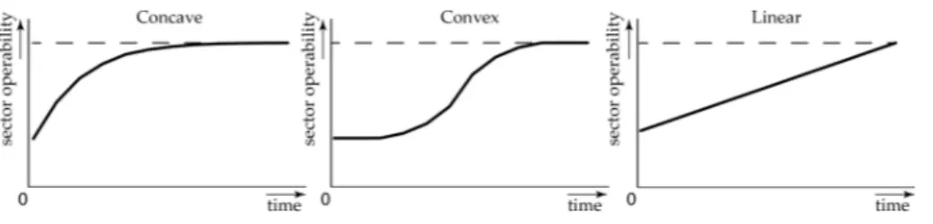
As identified in Sect. 2, an important characteristic which significantly influences the po-tential total losses is the duration of the recovery period and the type of recovery path. As shown in Fig. 2, we have defined three diﬀ_{erent paths: concave, convex and linear}

(similar paths have been used in Baghersad and Zobel, 2015). The concave recovery 15

path can be interpreted as being quick and smooth from the beginning, as a result of which most of the area is recovered within a couple of time steps. The convex path can be interpreted as delayed recovery. This may occur because emergency and re-pair activities are hampered. This implies slow recovery in the immediate post-disaster time periods and quicker recovery later. Finally, the linear recovery path is assumed to 20

be a “way through the middle” and based on the assumption that capital available for reconstruction is evenly distributed over the recovery period. Due to the large uncer-tainty in the potential recovery path and duration, it is worthwhile to test the results with these three recovery paths. In this exercise, we assume a full recovery in one year for all paths in all the models.

(15)

NHESSD

3, 7053–7088, 2015

E. E. Koks et al.

Title Page

Tables Figures

◭ ◮

Back Close

Full Screen / Esc

Discussion

P

a

per

|

Discussion

P

a

per

|

Discussion

P

a

per

|

Discussion

P

a

per

|

3.6 Data

For the ARIO and IEES model, the data is based on GTAP 8 (Global Trade Analysis Project) database (Narayanan et al., 2012) and ISTAT (Italian National Statistical Insti-tute) data. In order to get a sub-national database for each one of the 20 Italian regions and derive the bilateral trade flows between them, we integrate GTAP with information 5

stemming from ISTAT. We split the GTAP data for Italy by using the ISTAT shares on valued added, labor and land for each sector and Italian region. To reconstruct the re-gional domestic demand and bilateral intra-national trade flows we make use of ISTAT transport data. An extensive description of the methodology can be found in Standardi et al. (2014) and Carrera et al. (2015).

10

For the MRIA model, a regionalized version for Italy of the European interregional supply and use table is used, developed by PBL Netherlands Environmental Assess-ment Agency (Thissen et al., 2013). The table distinguishes twenty diﬀ_{erent Italian}

re-gions (NUTS2 level), 15 sectors and 59 products, allowing for a detailed disaster impact analysis. Supply and use tables contain more information compared to I-O tables since 15

the separate industries and commodities of the supply and use tables are combined in the I-O tables using one out of several standard assumptions about technologies.

4 Study area and asset losses

For the comparison, we consider two simulated floods in the Po river basin in North-ern Italy. As shown in Fig. 3, the two floods aﬀ_{ect the administrative regions of Veneto}

20

and Emilia-Romagna in the downstream part of the basin. The two flood events con-sidered in this study represent the result of a simulation produced by ARPA Emilia Romagna (Regional Agency for Environmental Protection). The exercise simulates two levee breach scenario around the municipality of Occhiobello, one on the southern and one on the northern levee. The southern breach inundates the Emilia Romagna region, 25

while the northern breach the Veneto region. The case study in Veneto and Emilia

(16)

NHESSD

3, 7053–7088, 2015

E. E. Koks et al.

Title Page

Tables Figures

◭ ◮

Back Close

Full Screen / Esc

Discussion

P

a

per

|

Discussion

P

a

per

|

Discussion

P

a

per

|

Discussion

P

a

per

magna is selected for their relevance in the Northern Italy economy. Although being simulated, the scenarios are not totally unrealistic. Occhiobello is famous for being the location where in 1951 Italy experienced one of the largest inundations on records. And the location is reported be one of the most vulnerable sections along the Po river levee system. In 1951 the levee breach (northern) inundated more than 100 000 ha of 5

urban and agriculture land in Veneto causing large economic losses and more than 100 causalities. The river discharge associated with the levee breach considered in this study correspond to the discharge recorded during the Po river 2000 flood, which was approximately the discharge recorded in 1951 (10 300 vs. 9750 m3s−1_{). The flood}

caused by a left-bank breach on the Po river levee aﬀ_{ects Veneto region. It results}

10

in inundation of mainly agricultural land and dispersed small settlements. The flood cased on right-bank breach of Po river levee aﬀ_{ects Emilia-Romagna. It results in}

sub-stantial flooding of industrial areas, in addition to agricultural and residential areas. Table 3 shows the result of the asset loss assessment, performed with the use of depth-damage curves2.

15

As can be seen from Table 3, asset losses are very similar for both flood scenar-ios. There are, however, important diﬀ_{erences in the composition of the losses. Firstly,}

asset losses within industrial areas are more than twice as large in Emilia-Romagna compared to Veneto. They account for amounts to 15 % of the total losses in Veneto and 35 % of the losses in Emilia-Romagna. Secondly, asset losses in urban areas are 20

76 % of the total asset losses for the flood in Veneto, whereas only 52 % for the flood in Emilia-Romagna. Finally, the asset losses in agricultural areas are 9 and 10 % of the total asset losses for, respectively, Veneto and Emilia-Romagna.

2

(17)

NHESSD

3, 7053–7088, 2015

E. E. Koks et al.

Title Page

Tables Figures

◭ ◮

Back Close

Full Screen / Esc

Discussion

P

a

per

|

Discussion

P

a

per

|

Discussion

P

a

per

|

Discussion

P

a

per

|

5 Results

Table 4 shows the total output losses in Italy for the two floods, the three models and the three recovery paths. The calculations with the ARIO model result in the highest losses for the whole of Italy, for both floods and for each recovery path. This is in line with expectations from previous literature where it is stated that IO models result in 5

higher estimates of losses (e.g. West, 1995; Rose, 2005). The IEES model has, as expected, the lowest output losses in almost every model setup. Only for the concave recover path for the flood in Veneto the losses in the MRIA model are slightly lower. This can be explained on a sectoral level: in the MRIA model, the extra reconstruction demand, which goes directly towards the construction sector, has a clear positive eﬀ_ect

10

on this sector. In the IEES model, this positive eﬀ_{ect is rather marginal. For the convex}

and linear recovery paths, the higher sectoral losses due to slower recovery largely outweigh this positive eﬀ_{ect in the MRIA model. The rigid and flexible versions of the}

IEES model show comparable results for Italy as a whole. Important to note here is that the diff_{erence between the two model only has e}ff_{ect on the spatial di}ff_erentiation

15

of the losses (see Fig. 4).

When comparing the diﬀ_{erent recovery paths, a concave recovery path clearly}

re-sults in the lowest losses in all models. The convex and linear paths show, compared to the concave recovery path, somewhat similar results. This large diﬀ_{erence can be}

explained by the fact that the concave path results in a relatively quick reconstruction of 20

the aﬀ_{ected area and thus lower output losses. For both the convex and linear recover}

paths, it will take much longer before most of the area is reconstructed (see Fig. 2). Table 5 shows the losses for the flooded regions region only. It is worth noting that in the aﬀ_{ected region the cross-model di}ﬀ_{erences are much smaller and strongly}

de-pend on the recovery path. From Table 4 it becomes apparent that the ARIO-estimated 25

losses for Italy as a whole are almost six times larger than the IEES – Flex model for the concave recovery path and the Veneto flood scenario (first row). When considering only the losses of the aﬀ_{ected region, this di}ﬀ_{erence is a only factor 0.2 (first row in}

(18)

NHESSD

3, 7053–7088, 2015

E. E. Koks et al.

Title Page

Tables Figures

◭ ◮

Back Close

Full Screen / Esc

Discussion

P

a

per

|

Discussion

P

a

per

|

Discussion

P

a

per

|

Discussion

P

a

per

Table 5). This implies that the largest diﬀ_{erences in outcome between the models are}

occurring in the multiregional eﬀ_{ects of the disaster. More specifically, this means that}

the assumptions regarding multiregional spillover eﬀ_{ects (whether or not substitution,}

additional imports or factor mobility) is an important determinant of the final outcomes. A closer look at the diﬀ_{erences for the a}ﬀ_{ected region in Table 5 show additional}

5

divergences between the models compared to Table 4. Firstly, in Table 4 the ARIO model always predicts the highest losses. In Table 5, however, this is only the case for the concave recover path for the Veneto flood event. In all other scenarios, the losses calculated by the MRIA and the IEES – Flex model are higher. This may imply that allowing for more flexibility in the model results in higher losses in the aﬀ_ected

10

region. In the MRIA model, this may be explained by the maximum regional capacity. Interestingly, for the whole of Italy this results in lower losses compared to the ARIO model because production is taken over in other regions (MRIA and Flex) pr price eﬀ_{ects (rigid), but for the a}ﬀ_{ected region this results in higher losses. In the IEES –}

Flex model, a similar process occurs with the movement of production factors to other 15

non-aﬀ_{ected regions (which are not possible in the IEES – Rigid).}

When comparing the spatial distribution of the losses across the three models for the concave recovery curve of the Emilia-Romagna flood (Fig. 4), we find some in-teresting results. Firstly, the two “IO-based” models (i.e. the ARIO and MRIA model) show large diﬀ_{erences in the spatial distribution of losses. Whereas the ARIO model}

20

shows negative results in all regions, the MRIA model only shows negative results in the aﬀ_{ected region. What is notable is that the losses in the a}ﬀ_{ected region are higher}

in the MRIA model (as also shown in Table 5). As such, by allowing for substitution between producers in the model, the aﬀ_{ected region is a}ﬀ_{ected more heavily, while the}

non-aﬀ_{ected regions benefit. This can be explained by the ine}ﬃ_{ciency losses, which}

25

(19)

NHESSD

3, 7053–7088, 2015

E. E. Koks et al.

Title Page

Tables Figures

◭ ◮

Back Close

Full Screen / Esc

Discussion

P

a

per

|

Discussion

P

a

per

|

Discussion

P

a

per

|

Discussion

P

a

per

|

eﬀ_{ects in almost all non-e}ﬀ_{ected regions. The flexible version on the other hand shows,}

similar to the MRIA model, benefits in all other regions due to substitution eﬀ_ects.

Figure 5 shows a comparison of the results presented in Table 4 (the left boxplots for Veneto and Emilia-Romagna in Fig. 5) with the same modelling setup but without additional reconstruction demand due to the disaster (the right boxplots for the two sce-5

narios). The figure shows that not considering reconstruction demand in the model not only results in higher losses, but also in a larger diﬀ_{erence in losses between the}

sev-eral recovery curves within one flood scenario. The diﬀ_{erence can be addressed to the}

increase in production (and thus increase in value added) due to the increased recon-struction demand from the aﬀ_{ected sectors towards the construction sector. Important}

10

to note is that mainly the outliers change; for both the Veneto and Emilia-Romagna scenario, the median losses remain almost the same between the reconstruction and no reconstruction methods. From Fig. 5 we can interpret that especially with higher losses and slower recovery (the highest losses occur, as can be seen in Table 4, in the convex and linear recovery curves), including reconstruction demand will substantially 15

reduce the total output losses.

6 Discussion

In our comparison exercise the ARIO model, but also traditional multiregional IO mod-els in general, are lacking the capacity to estimate the potential substitution eﬀ_{ects in}

other regions. This can be seized in CGE or (non)-linear programming methods, as 20

shown by the MRIA and IEES model. Due to the linearity of IO models, other regions always yield losses, which is consistent with results in MacKenzie et al. (2012) and In den Bäumen et al. (2015). But this is contrary to the expected gains in non-aﬀ_ected

regions around the aﬀ_{ected area (see e.g. Albala-Bertrand, 2013). Hence it is highly}

unlikely that all regions will suﬀ_{er losses. On the other hand, it is in a real situation also}

25

unlikely that substitution in products between regions is possible without any barriers to trade and movements, of production factors. Therefore, the “truth” might be

(20)

NHESSD

3, 7053–7088, 2015

E. E. Koks et al.

Title Page

Tables Figures

◭ ◮

Back Close

Full Screen / Esc

Discussion

P

a

per

|

Discussion

P

a

per

|

Discussion

P

a

per

|

Discussion

P

a

per

where in the middle of the results. To get a better picture of substitution possibilities in the aftermath of a disaster, more empirical studies should analyze the post-recovery process in high-income countries.

The recovery path and reconstruction demand are proven to be important factors in the estimation of total output losses. This is not only observed in this study, but also in 5

studies of Baghersad and Zobel (2015), Hallegatte (2008, 2014) and Koks et al. (2015). Results show that both the duration and the type of recovery path can significantly alter the model outcomes. Unfortunately, as mentioned in Sect. 2, almost no empirical data is available to calibrate which duration and which path is suitable for which size and type of disaster. Therefore, more empirical research is required in obtaining this information 10

to further improve the use of the recovery path in disaster impact modelling. It should be noted that, even without this empirical calibration, recovery paths should be used in disaster impact modelling.

A better understanding of production losses is important for public budgeting, as well as for private resilience choices. On the public income side, a drop in production im-15

plies lower tax proceeds and other revenues in the current, and possibly in the future accounting periods. Even if the production is restored quickly, the losses of aﬀ_ected

firms can influence state revenues through tax deductions conceded in the subse-quent periods. On the spending side, post-disaster recovery programs and restoration of public infrastructure inure financial obligations which may increase government debt. 20

Unfolded through cumulative or cascading paths, a series of medium-sized disasters or single large disasters may produce or aggravate existing economic imbalances and expand disparities across states or regions. It would be wise to consider economic risk embodied in natural hazards as a liability. The European Cohesion Policy measures states’ economic performance using gross domestic/regional product (GDP/GRP), and 25

(21)

sol-NHESSD

3, 7053–7088, 2015

E. E. Koks et al.

Title Page

Tables Figures

◭ ◮

Back Close

Full Screen / Esc

Discussion

P

a

per

|

Discussion

P

a

per

|

Discussion

P

a

per

|

Discussion

P

a

per

|

idary financial assistance through the European Solidarity Fund (EUSF). In this context the threshold is specified as a ratio of structural damage to GNI or GRP. In principle, the solidarity payments would be better targeted if triggered by the post-disaster drops in GNI/GRP or public revenues collected. The recent advancements in economic risk assessment, as presented in this paper, make it possible to base similar decisions on 5

a sound and robust knowledge.

7 Concluding remarks

In this study we have analyzed several risk scenarios in a pilot study area using three regional economic models: two hybrid multiregional IO models (ARIO and MRIA) and a regionally disaggregated instance of a global CGE model (IEES). The pilot study area 10

is located in the downstream part of the Po river. The two flood scenarios comprise levee breaks on a Po river levee at the same place where it occurred in 1951. The economic losses for the flood scenarios have been calculated for all three models, using three diﬀ_{erent recovery paths (concave, convex and linear).}

Relatively large diﬀ_{erences in model outcomes have been found on the national scale}

15

for all flood scenarios and considered recover paths. The most substantial diﬀ_erences

were found between the ARIO model on the one hand and the MRIA and the IEES model on the other hand (results vary by up to a factor of seven). Diﬀ_{erences between}

the MRIA and the IEES model were relatively minor, whereas the results of the ARIO model were approximately three to six times higher compared to the results of the IEES 20

model. The main reason for this diﬀ_{erence is the linear structure assumed in the ARIO}

model and its complete lack of substitution in production, trade or products. Due to the linear characteristics of the model, all other (non-aﬀ_{ected) regions will be negatively}

aﬀ_{ected due to the disaster. We argue that this negative e}ﬀ_{ect for all other regions}

is not realistic and, therefore, we suggest that multiregional disaster impact studies 25

should apply more flexible economic models such as the MRIA or IEES model.

(22)

NHESSD

3, 7053–7088, 2015

E. E. Koks et al.

Title Page

Tables Figures

◭ ◮

Back Close

Full Screen / Esc

Discussion

P

a

per

|

Discussion

P

a

per

|

Discussion

P

a

per

|

Discussion

P

a

per

The diﬀ_{erent recovery paths showed that the speed of recovery is crucial for the total}

losses. A quick recovery (a concave recovery path) results in substantial lower losses compared to a slow recovery (convex recovery path). This outcome is observed in all three models. The empirical research on this, however, is rather limited. As such, future research is required to explore which recovery paths are empirically observed and 5

what resilience measures are required to make sure an aﬀ_{ected area will be recovered}

quickly to reduce losses. We argue that solutions could be explored in the field of public-private partnerships.

This study showed that some model outcomes are susceptible to underlying assump-tions, while others are not. Therefore, for a detailed assessment of disaster impacts on 10

economy, including the price eﬀ_{ects and e}ﬀ_{ects on employment, the CGE models are}

better suited. For assessing cost-benefit ratio of specific resilience measures, both the MRIA and the IEES model seems to be equally useful and produce similar outcomes in terms of output losses. The conventional multiregional IO models may largely overes-timate the losses. For future research, more empirical data is needed to better explore 15

the trade-oﬀ_{between the analyzed models.}

Acknowledgements. The research underlying this paper has received funding from the EU’s Seventh Framework Programme (FP7/2007–2013) under grant agreement No. 308438 (EN-HANCE – Enhancing risk management partnerships for catastrophic natural hazards in Eu-rope), grant agreement No. 282834 (TURAS – Transitioning towards urban resilience and

sus-20

tainability), grant agreement No. 603396 (RISES-AM – Responses to coastal climate change: Innovative Strategies for high End Scenarios – Adaptation and Mitigation) and grant agreement No. 609642 (ECOCEP – Economic modelling for ClimateEnergy Policy), the Italian Ministry of Education, University and Research and the Ministry for Environment, Land and Sea (the GEMINA project) and NWO VICI grant agreement No. 45314006. The paper is supported by

25

(23)

NHESSD

3, 7053–7088, 2015

E. E. Koks et al.

Title Page

Tables Figures

◭ ◮

Back Close

Full Screen / Esc

Discussion

P

a

per

|

Discussion

P

a

per

|

Discussion

P

a

per

|

Discussion

P

a

per

|

References

Albala-Bertrand, J. M.: Disasters and the Networked Economy, Routledge, London, UK, 2013. Baghersad, M. and Zobel, C. W.: Economic impact of production bottlenecks caused by

disasters impacting interdependent industry sectors, Int. J. Prod. Econ., 168, 71–80, doi:10.1016/j.ijpe.2015.06.011, 2015.

5

Bockarjova, M.: Major disasters in modern economies: an input-output based approach at mod-elling imbalances and disproportions, University of Twente, Twente, the Netherlands, 2007. Carrera, L., Standardi, G., Bosello, F., and Mysiak, J.: Assessing direct and indirect economic

impacts of a flood event through the integration of spatial and computable general equilibrium modelling, Environ. Modell. Softw., 63, 109–122, 2015.

10

Cavallo, E. and Noy, I.: The Economics of Natural Disasters: A Survey, Inter-American Devel-opment Bank Working Paper No. 124, Inter-American DevelDevel-opment Bank, 2009.

Cho, S., Gordon, P., Moore, I. I., James, E., Richardson, H. W., Shinozuka, M., and Chang, S.: Integrating transportation network and regional economic models to estimate the costs of a large urban earthquake, J. Regional Sci., 41, 39–65, 2001.

15

Ciscar, J. C., Feyen, L., Soria, A., Lavalle, C., Raes, F., Perry, M., Nemry, F., Demirel, H., Roz-sai, M., Dosio, A., Donatelli, M., Srivastava, A., Fumagalli, D., Niemeyer, S., Shrestha, S., Ciaian, P., Himics, M., Van Doorslaer, B., Barrios, S., Ibáñez, N., Forzieri, G., Rojas, R., Bianchi, A., Dowling, P., Camia, A., Libertà, G., San Miguel, J., de Rigo, D., Caudullo, G., Barredo, J.-I., Paci, D., Pycroft, J., Saveyn, B., Van Regemorter, D., Revesz, T., Vandyck, T.,

20

Vrontisi, Z., Baranzelli, C., Vandecasteele, I., e Silva, F., and Ibarreta, D.: Climate impacts in Europe. Results from the JRC PESETA II project, JRC Scientific and Policy Reports, EUR 26586EN, 2014.

Cobb, C. W. and Douglas, P. H.: A theory of production, Am. Econ. Rev., 18, 139–165, 1928. Crowther, K. G. and Haimes, Y. Y.: Application of the inoperability input–output model (IIM) for

25

systemic risk assessment and management of interdependent infrastructures, Syst. Eng., 8, 323–341, 2005.

Hallegatte, S.: An adaptive regional input-output model and its application to the assess-ment of the economic cost of Katrina, Risk Anal., 28, 779–799, doi:10.1111/j.1539-6924.2008.01046.x, 2008.

30

Hallegatte, S.: Modeling the role of inventories and heterogeneity in the assessment of the economic costs of natural disasters, Risk Anal., 34, 152–167, 2014.

(24)

NHESSD

3, 7053–7088, 2015

E. E. Koks et al.

Title Page

Tables Figures

◭ ◮

Back Close

Full Screen / Esc

Discussion

P

a

per

|

Discussion

P

a

per

|

Discussion

P

a

per

|

Discussion

P

a

per

Hertel, T. W.: Global Trade Analysis: Modeling and Applications, Cambridge University Press, Cambridge, UK, 1997.

Hu, A., Xie, W., Li, N., Xu, X., Ji, Z., and Wu, J.: Analyzing regional economic impact and resilience: a case study on electricity outages caused by the 2008 snowstorms in southern China, Nat. Hazards, 70, 1019–1030, 2014.

5

in den Bäumen, H. S., Többen, J., and Lenzen, M.: Labour forced impacts and production losses due to the 2013 flood in Germany, J. Hydrol., 527, 142–150, doi:10.1016/j.jhydrol.2015.04.030, 2015.

IPCC: Managing the Risks of Extreme Events and Disasters to Advance Climate Change Adaptation: Special Report of the Intergovernmental Panel on Climate Change, edited by:

10

Field, C. B., Barros, V., Stocker, T. F., Qin, D., Dokken, D. J., Ebi, K. L., Mastrandrea, M. D., and Mach, K. J., Cambridge University Press, Cambridge, UK, New York, NY, USA, p. 582, 2012.

Jongman, B., Kreibich, H., Apel, H., Barredo, J. I., Bates, P. D., Feyen, L., Gericke, A., Neal, J., Aerts, J. C. J. H., and Ward, P. J.: Comparative flood damage model assessment: towards a

15

European approach, Nat. Hazards Earth Syst. Sci., 12, 3733–3752, doi:10.5194/nhess-12-3733-2012, 2012.

Kim, T. J., Ham, H., and Boyce, D. E.: Economic impacts of transportation network changes: implementation of a combined transportation network and input-output model, Pap. Reg. Sci., 81, 223–246, 2002.

20

Koks, E. E. and Thissen, M.: The economic-wide consequences of natural hazards: an appli-cation of a European interregional input-output model, Conf. Pap. 22nd Input Output Conf., 14–18 July 2014, Lisboa, Portugal, 2014.

Koks, E. E., Boč_{karjova, M., De Moel, H., and Aerts, J. C. J. H.: Integrated direct and} in-direct flood risk modeling: development and sensitivity analysis, Risk Anal., 35, 882–900,

25

doi:10.1111/risa.12300, 2015.

MacKenzie, C. A., Santos, J. R., and Barker, K.: Measuring changes in international production from a disruption: case study of the Japanese earthquake and tsunami, Int. J. Prod. Econ., 138, 293–302, doi:10.1016/j.ijpe.2012.03.032, 2012.

Merz, B., Kreibich, H., Schwarze, R., and Thieken, A.: Review article ”Assessment of economic

30

(25)

NHESSD

3, 7053–7088, 2015

E. E. Koks et al.

Title Page

Tables Figures

◭ ◮

Back Close

Full Screen / Esc

Discussion

P

a

per

|

Discussion

P

a

per

|

Discussion

P

a

per

|

Discussion

P

a

per

|

Narayanan, B. G. and Walmsley, T. L.: Global trade, assistance, and production: the GTAP 7 data base, Center for Global Trade Analysis, Purdue University, Australia, 134, 2008. Okuyama, Y.: Economics of natural disasters: a critical review, Res. Pap., 12, 20–22, 2003. Okuyama, Y.: Globalization and localization of disaster impacts: an empirical examination,

CE-Fifo Forum, 11, 56–66, 2010.

5

Okuyama, Y.: Disaster and economic structural change: case study on the 1995 kobe earth-quake, Econ. Syst. Res., 26, 98–117, doi:10.1080/09535314.2013.871506, 2014.

Okuyama, Y. and Chang, S. E.: Modeling Spatial and Economic Impacts of Disasters, Springer, New York, 324 pp., 2004.

Okuyama, Y. and Sahin, S.: Impact Estimation of Disasters: A Global Aggregate for 1960 to

10

2007, World Bank, available at: https://openknowledge.worldbank.org/handle/10986/4157 (last access: 20 November 2015), 2009.

Okuyama, Y. and Santos, J. R.: Disaster impact and input-output analysis, Econ. Syst. Res., 26, 1–12, 2014.

Okuyama, Y., Hewings, G. J. D., and Sonis, M.: Measuring economic impacts of disasters:

15

interregional input-output analysis using sequential interindustry model, in: Modeling Spatial and Economic Impacts of Disasters, Springer, New York, 77–101, 2004.

Park, J., Cho, J., Gordon, P., II, J. E. M., Richardson, H. W., and Yoon, S.: Adding a freight net-work to a national interstate input–output model: a TransNIEMO application for California, J. Transp. Geogr., 19, 1410–1422, doi:10.1016/j.jtrangeo.2011.07.019, 2011.

20

Rose, A.: Input-output economics and computable general equilibrium models, Struct. Change Econ. Dynam., 6, 295–304, 1995.

Rose, A.: Economic principles, issues, and research priorities in hazard loss estimation, in: Modeling Spatial and Economic Impacts of Disasters, Springer, New York, 13–36, 2004. Rose, A. and Liao, S.-Y.: Modeling regional economic resilience to disasters: a computable

gen-25

eral equilibrium analysis of water service disruptions*, J. Regional Sci., 45, 75–112, 2005. Rose, A. and Wei, D.: Estimating the economic consequences of a port shutdown: the special

role of resilience, Econ. Syst. Res., 25, 212–232, 2013.

Rose, A., Benavides, J., Chang, S. E., Szczesniak, P., and Lim, D.: The regional economic im-pact of an earthquake: direct and indirect eﬀ_{ects of electricity lifeline disruptions, J. Regional}

30

Sci., 37, 437–458, 1997.

Santos, J. R. and Haimes, Y. Y.: Modeling the demand reduction input-output (I-O) inoperability due to terrorism of interconnected infrastructures*, Risk Anal., 24, 1437–1451, 2004.

(26)

NHESSD

3, 7053–7088, 2015

E. E. Koks et al.

Title Page

Tables Figures

◭ ◮

Back Close

Full Screen / Esc

Discussion

P

a

per

|

Discussion

P

a

per

|

Discussion

P

a

per

|

Discussion

P

a

per

Seung, C. K.: Measuring spillover eﬀ_{ects of shocks to the Alaska economy: an} inter-regional social accounting matrix (IRSAM) model approach, Econ. Syst. Res., 26, 224–238, doi:10.1080/09535314.2013.803039, 2014.

Shibusawa, H., Yamaguchi, M., and Miyata, Y.: Evaluating the impacts of a disaster in the Tokai Region of Japan: a dynamic spatial CGE model approach, Stud. Reg. Sci., 39, 539–551,

5

2009.

Standardi, G., Bosello, F., and Eboli, F.: A sub-national version of the GTAP model for Italy, Work. Pap. Fondazione Eni Enrico Mattei, CMCC, Venice, 1–20, 2014.

Taylor, L. and Lysy, F. J.: Vanishing income redistributions: keynesian clues about model sur-prises in the short run, J. Dev. Econ., 6, 11–29, 1979.

10

Thissen, M.: The indirect economic eﬀ_{ects of a terrorist attack on transport infrastructure: a} pro-posal for a SAGE, Disaster Prev. Manag., 13, 315–322, 2004.

Thissen, M. and Lensink, R.: Macroeconomic eﬀ_{ects of a currency devaluation in Egypt: an} analysis with a computable general equilibrium model with financial markets and forward-looking expectations, J. Policy Model., 23, 411–419, 2001.

15

Thissen, M., van Oort, F., Diodato, D., and Ruijs, A.: Regional Competitiveness and Smart Specialization in Europe: Place-Based Development in International Economic Networks, Edward Elgar Publishing, Cheltenham, UK, 2013.

Tsuchiya, S., Tatano, H., and Okada, N.: Economic loss assessment due to railroad and high-way disruptions, Econ. Syst. Res., 19, 147–162, doi:10.1080/09535310701328567, 2007.

20

UNISDR: Sendai Framework for Disaster Risk Reduction, UNISDR, Geneva, 2015–2030, 2015.

(27)

NHESSD

3, 7053–7088, 2015

E. E. Koks et al.

Title Page

Tables Figures

◭ ◮

Back Close

Full Screen / Esc

Discussion

P

a

per

|

Discussion

P

a

per

|

Discussion

P

a

per

|

Discussion

P

a

per

|

Table 1.Comparison of IO and CGE approach on important modelling characteristics.

Characteristic IO CGE

Time horizon Short-run Short-, medium and long-run Substitution Not possible in traditional model Possible

Mathematical complexity Linear/simple Non-linear/advanced

Model type Partial economic analysis General equilibrium (system) eﬀ_ects.

Supply side Lack of resource constraints Handles supply constraints Sector interdependencies Accounted for via technical coeﬃ_cients _{Accounted for via (cross)elasticities}

Resilience Generally under recognized Primarily price mechanism Estimation accuracy Overestimation of disaster impact Underestimation of disaster impact