Imaginary Money
Eduardo Loyo
∗John F. Kennedy School of Government
Harvard University
[email protected]
This Version: April 10, 2001
First Draft: March 1, 2001
Abstract
This paper considers price setting in pure units of account, linked to the means of payment through managed parities. If prices are sticky in the units in which they are set, parity changes may facilitate equilibrium adjustment of relative prices. The paper derives simultaneously the opti-mal choice of unit of account by each price setter, and the optiopti-mal parity policy. The gains from having multiple units of account are computed for a simple calibrated economy.
1
Introduction
The salary is 2,000 livres a year, but I should have to spend six months at Versailles and other six in Paris, or wherever I like. I do not think that I shall accept it, but I have yet to hear the advice of some good friends on the subject. After all, 2,000 livres is not such a big sum. It would be so in German money, I admit, but here it is not. It amounts to 83 louis d’or, 8 livres a year - that is, to 915 florins, 45 kreuzer in our money (a considerable sum, I admit), but here worth only 333 thalers, 2 livres -which is not much. It is frightful how quickly a thaler disappears here.
W.A. Mozart, 1778.
Think for a moment about the monetary architecture of medieval and early modern Europe. Whatfirst comes to mind is a world with very porous mon-etary borders, and in each political jurisdiction a sovereign busy at debasing
the metallic content of local coinage. That alone spanned a variety of possible standards of value, which could be based either on a fixed weight of precious metal or on afixed tally of circulating coins, local or foreign. But there was a lesser known twist to the monetary standards of the time: the use of units of account separate from the means of payment, without any sort of physical embodiment, and simply defined by legal tender parities with respect to the means of payment. These parities changed over time, making the disembodied units of account more than mere aliases for fixed multiples or fractions of ex-isting means of payment. Einaudi (1936) aptly termed such units of account ‘imaginary money’.
Economic historians disagree about the extent to which imaginary monies really enjoyed a life of their own: how widespread was their use as alternative units of account, and how variable were their parities with respect to ‘real’ monies, the means of payment?1 Regardless of the historical verdict, imaginary monies - disembodied units of account whose parity with respect to the medium of exchange can be varied at will - remain a tantalizing logical possibility.
Separation between the monetary functions of unit of account and means of payment has been a traditional theme of monetary futurology (see, for in-stance, Cowen and Kroszner, 1994), as has the possibility of multiple monetary standards within a given geographical area (Cohen, 1998, 1999, 2000). But that literature has focused on sweeping transformations in the ‘anchoring’ of the gen-eral price level - in particular, in the role of the means of payment. The same applies to the debate over private issuance of substitutes to base money within any given monetary standard, and its consequences for the conduct of monetary policy.2 Scant thought has been given to a scheme predicated on more modest changes in the transaction settlement technology: retain a unique standard for the exchange medium, somehow under government control; as additional policy instruments, introduce imaginary monies defined by reference to the medium of exchange, to serve as alternative units of account.
A modern day motivation for interest in imaginary monies can be offered by analogy with Milton Friedman’s (1953) classic argument for floating exchange rates: if shocks require relative price changes but there is some nominal rigidity, prices could be nudged in the right direction by manipulating the parity between the units of account in which they are set. Interim price misalignment and the ensuing misallocation of resources would thus be mitigated. As larger and larger areas of the world opt for unification of means of payment, imaginary monies, if they could be made to catch on as pricing units, would be a way of reintroducing valuable degrees of freedom to respond to relative price shocks. Of course, one must weigh the calculation burden inherent to multiple units of account against the reduction in price misalignment, in order to arrive at the net welfare gain from imaginary monies.
Just as monetary futurology has been heralding the age of non-territorial, self-organizing networks of users of different means of payment, here I consider
1See, for instance, Bloch (1934), Cipolla (1956, 1982, 1991), Einaudi (1936, 1937), Lane
and Mueller (1985), and van Werveke (1934).
the possibility of producers choosing by themselves among units of account for pricing, perhaps on grounds other than locational. It would make sense for producers whose idiosyncratic cost or demand shocks are highly correlated to price together in a separate unit of account, if they could count on parity policy to facilitate their desired relative price adjustment with respect to the rest of the economy. Sectoral links may even dominate location as a source of correlation across shocks. It is the self-organizing (and potentially non-territorial) aspect of the scheme, besides the separation between units of account and means of payment, that sets it apart from the conventional problem of optimal currency areas.
This paper is an attempt toflesh out formally the intuitive case for imaginary monies.3 I consider the simplest example of a single imaginary money on top of the real money. In section 2, a fairly standard general equilibrium macroeco-nomic model with sticky prices is augmented to incorporate the optimal choice of pricing unit by individual producers, which is derived simultaneously with the optimal policy towards the imaginary money parity. In section 3, I calibrate the model tofind quantitative estimates of the drop in price misalignment and its welfare benefit, to be weighed against one’s best guess of the calculation burden entailed by multiple units of account. Section 4 concludes, pointing to key caveats to the analysis performed in the paper and indicating directions for refinement and further research.
2
An economy with imaginary money
2.1
Basic setup and notation
Consider an economy where prices can be quoted in either one of two units of account. The first is the usual standard of value, the circulating means of payment, to which I refer as thereal money(abbreviatedr$). The second, which I callimaginary money(abbreviatedi$), is a pure unit of account, without any physical representation and defined by no more than an officially announced parity X with respect to the real money: i$X = r$1 (an increase in X is a ‘devaluation’ of the imaginary money).
The economy contains a continuum of differentiated goods indexed by the unit interval. If goodzhas its price posted in terms of real money, say atr$P(z),
3The themes explored here made an incipient appearance in a couple of pages of Cowen
an equivalent price in imaginary money could be readily calculated asi$XP(z). Conversely, if goodz has its price posted in terms of imaginary money, say at
i$Q(z), that is understood as willingness to trade the good for an amount QX(z) of real money. So, for any good z, I denote byP(z)its price in terms of real money, and by Q(z) its price in terms of imaginary money; these prices are related throughQ(z) =XP(z).
Each differentiated good is produced by a monopolistically competitivefirm, which turns homogeneous laborh(z)into outputc(z)according to the simple production function:
c(z) = h(z)
s(z) (1)
Increases in s(z) are adverse cost shocks: more labor becomes necessary to produce a unit of goodz.
The economy is inhabited by a representative household with preferences described by a utility function u(c, h), increasing in c and decreasing in h. Consumption enters through to the CES index:
c≡
1
Z
0
c(z)1/µdz
µ
where µµ−1 is the elasticity of substitution across goods, andµ >1is a measure of the market power created by the preference for variety. Meanwhile:
h≡
1
Z
0
h(z)dz
is the aggregate amount of work employed in the economy.
The representative household should allocate expenditures across the diff er-entiated goods in order to minimize the cost of obtaining a unit of the CES aggregator:
min
1
Z
0
P(z)c(z)dz
s.t.
1
Z
0
c(z)1/µdz
µ
=c
which results in the following demand functions for each good:
c(z) =cp(z)1−µµ (2)
wherep(z)≡ PP(z) is the real price of goodz, since:
P ≡
1
Z
0
P(z)1−1µ dz
is the general price level in this economy - i.e., the price of a unit ofcobtained as an expenditure minimizing bundle:
1
Z
0
P(z)c(z)dz=P c
A similar price index could be calculated in terms ofi$:
Q=
1
Z
0
Q(z)1−1µ dz
1−µ
Because they are homogeneous of degree one, these price indices inherit the law of one price that holds for each individual good: Q=XP. Working in either denomination, one computes the same real price for each good: QQ(z) = PP(z) = p(z).
The representative household maximizes utility by satisfying the following marginal condition:
uc(c, h)w=−uh(c, h) (3)
wherewis the real wage rate.
It is convenient to define an aggregate index of labor requirements for pro-duction, with the same weighting as the aggregate price indices:
s≡
1
Z
0
s(z)1−1µdz
1−µ
From the demand functions derived above and the specification of technology, it follows that:
h=csδ (4)
where:
δ≡
1
Z
0
s(z) s p(z)
µ
1−µdz
The latter expression can be interpreted as a coefficient of relative price mis-alignment. It attains its minimal value of unity whenp(z) =s(sz) for allz, that is, when all prices are aligned in proportion to costs.
Suppose for now that allfirms set their prices with full knowledge of the cost conditions. In real terms, their profit maximization can be described by:
max
p(z)[p(z)−s(z)w]cp(z) µ
1−µ
which is solved byp(z) =µs(z)w. Integrating this pricing rule over all z, one
enjoy market power and set prices by applying the mark-upµ >1over marginal costs, the equilibrium level of activity is lower than would be socially desirable. That reflects the lowering of the equilibrium real wage by the exercise of market power.4 However, this equilibrium involves no relative price misalignment, as
p(z) = s(sz) for allz, and soδ= 1.
The model does not include shocks to preferences. In the world of constant desired mark-ups just described, changes in preferences (say, scaling up or down the contribution of each individualc(z) to thecindex) could only affect equi-librium relative prices through their effect on the marginal costs of production, as market clearing quantities change and the producers slide along their given marginal cost curves. Assuming that the marginal cost curves are horizontal, as I have done in (1), completely shuts down that channel. As a result, shocks to preferences would add nothing of central interest to the issues at stake here.5 Since the greatest loss of generality so far stems from the assumption of constant marginal cost curves, it would be nice if one could regard that as a re-alistic feature of the economy, against the full weight or received microeconomic wisdom. Blinder et al. (1998) report evidence that most firms (almost 90% of their sample) perceive their marginal cost curves as eitherflat or decreasing over the range that matters for cyclicalfluctuations. They interpret thatfinding as supportive of Hall’s (1986, 1988) conjecture that marginal costs vary little over the cycle, or rather of Ramey’s (1991)findings of countercyclical marginal costs. But Blinder et al. recognize that industry executives may have confused marginal with average (including averagefixed) costs in answering their survey question. The latest evidence in favor of procyclical marginal costs can be found in Rotemberg and Woodford (1999b), although some of that procyclicality can presumably be billed to aggregate factor scarcity rather than being a property internal to each firm’s marginal cost curve. Anyway, I maintain throughout the theoretical derivation of this section the simplifying assumption of constant marginal cost curves, and leave its consequences for the normative implications of the model to be briefly discussed in the conclusion.
2.2
Minimizing price misalignment
In its own right, price misalignment is bad for social welfare. It increases the aggregate work effort hrequired to obtain any given amount of the CES con-sumption index, or, conversely, it reduces the amount ofcobtained from a given aggregate work effort. The reason is that consumption concentrates on goods that are relatively cheaper to buy, though not so much cheaper to produce,
4The command optimum in aggregate variables (still leaving households free to choose the
composition of the consumption bundle, according to relative prices) would involve maximizing
u(c, h)subject to h = csδ, for which the first order conditions would include δ = 1 and
uc(c, h) = −uh(c, h)s. In the decentralized equilibrium, condition (3) implies uc(c, h) =
−uh(c, h)sµ, resulting in a lower level of activity. If the equilibrium real wage werew = 1s
instead ofw= 1
sµ, (3) would yield the command optimum level of activity.
5Of course, insofar as they change equilibrium quantities, shocks to preferences would
causing the consumption bundle to deviate from the optimal variety across dif-ferentiated goods. The socially optimal consumption bundle should satisfy, for every pair of goods, equality between the ratios of marginal utilities and of mar-ginal costs. But the demanded consumption bundle will instead equate marmar-ginal utility ratios to relative prices. If relative prices are not aligned with relative marginal costs, the allocation of consumption will not be optimal.
If we were preparing to consider a command optimum in aggregate quanti-ties, with a social planner arbitrarily choosing c, hand δ, given s, in order to maximize the representative household’s utility subject only to (4), but leaving the household free to allocate consumption expenditures in response to rela-tive prices, then policy would necessarily involve minimizingδ. That does not mean, however, that an enlightened policymaker attempting to implement the best possible decentralized equilibrium ought to minimize price misalignment, unless one can do so without affecting the equilibrium real wage. Theδ-reducing policies examined below will actually impact the equilibrium real wage in one way or another. If, without any intervention onδ, the economy would be oper-ating below its efficient level of activity, then lowerδaccompanied by higherw
should be welcome. But, if the reduction inδis accompanied by a large enough fall inw, the welfare effects could be negative.
Yet there are assumptions under which aδ-minimizing policy will invariably select the best decentralized equilibrium. For instance, if (3) is such that changes insδ and w get reflected either in equilibrium consumption or in equilibrium hours of work, but not both, then a policy of minimizing price misalignment will be optimal. This is because minimization of δ will be equivalent, in one extreme, to minimizing the effort necessary to obtain theconstant equilibrium level of consumption, which can only make households better off; and likewise in the other extreme, where it will be certain to improve social welfare by maximizing the level of consumption allowed by theconstant equilibrium level of employment.6
It is easy to specify families of utility functions for which that property can be arbitrarily well approximated with limiting choices of parameters. Take for instance the Cobb-Douglas functionu(c, h) = (c−c∗)β(h∗−h)1−β, where
c∗ can be interpreted as a minimum tolerable level of consumption and h∗ as a maximum tolerable work effort, and 0 < β < 1. As β → 0, all variation concentrates in employment, andu(c, h)→h∗−c∗sδ in equilibrium, which is maximized by minimizingδ. In the opposite extreme, β →1 concentrates all variation in consumption, andu(c, h)→h∗
sδ −c∗ in equilibrium, which is again maximized by minimizingδ.
In this paper, I focus on cases such as those. The limiting parametrizations of the Cobb-Douglas are mere examples of utility functions with the desired properties. No further reference to the form of the utility function will be nec-essary, and all the results below apply to any specification that shuts down all equilibrium variation of either consumption or employment. Of course, this
6In this case,neithercnor hcan vary in response to changes inwalone: without changes
modeling strategy is chosen for expositional clarity rather than realism. The idea is to focusfirst on the most direct channel for imaginary money to improve welfare, namely, reducing price misalignment and making theallocation of pro-duction across goods more efficient. Additional general equilibrium effects are left for future research.
It is worth mentioning that all the caveats in this subsection matter only if one cares, for positive purposes, about assuming that policymakers guide their policy actions by the welfare of the inhabitants of the economy, and, for nor-mative purposes, about evaluating alternative policy regimes according to that same criterion. All the results below are generally valid as positive statements about how private agents would respond to a policy of minimizing price mis-alignment, and about the degrees of misalignment and allocative inefficiency that would ultimately result.
2.3
Cost shocks and price rigidities
Iffirms could set prices with full knowledge of costs, there would be no reason for concern about price misalignment. Price misalignment becomes a concern as a consequence of nominal price rigidities: prices that are set before the costs are fully known may end up out of line. Prices might be set in either real or imaginary money, and the parity between the two units of account can be manipulated to bring prices closer to alignment, once costs are realized. But
firms should take these possible movements in the parity, and their general equilibrium effects, all into account when choosing what currency to set prices in, and what prices to post.
I consider this problem formally in a static model with a single market period. In the runup to the market period, events unfold in the following order: (i) First, each firm chooses between setting prices in r$ and i$, and posts a price in its preferred unit of account; (ii) The values ofs(z)realize for allfirms, from a known probability distribution; (iii) Observing the realized{s(z)}, and what firms set prices in what unit of account, the government sets the parity
X, while it also sets monetary policy instruments (not explicitly modeled) in such a way as to deliver a certain general price level in real moneyP; (iv) A fraction α of the firms is randomly selected (as in Calvo, 1983) to post new prices, incorporating all information already revealed, and everyfirm must then satisfy all forthcoming demand at their posted prices.7 In step (i),firms must take into account what they anticipate for{s(z)},X andP.
The analysis of the problem is considerably facilitated if performed with an approximation to the model. One mustfirst choose a benchmark around which to approximate. A natural choice is aflex-price equilibrium in which all goods require the same labor inputs(z) =s. In that equilibrium, all prices will also be equal, and there will be no price misalignment. The marginal distribution
7Lest there should be confusion, note that myαis Calvo’s1−α. Calvo’s device was meant
of eachs(z) is assumed to be the same for everyz, with means. As a result
b
s(z) ≡ s(zs)−s has mean zero for all z. Denoting bs ≡ s−ss, up to afirst order approximation this can be calculated according to:
b s=
1
Z
0
b
s(z)dz (5)
and so, up to afirst order approximation,Ebs= 0as well. For a generic variable
y, I shall denote byy its value at the benchmark equilibrium, andyb≡y−yy. From the definition of the coefficient of price misalignment, one can verify that, in a neighborhood of the benchmark equilibrium, and up to afirst order approximation,bδ= 0. In other words, price misalignment is not afirst order phenomenon, and can only be studied with higher order approximations to the model. Price misalignment achieved an earlier notoriety amid the debate over the costs of inflation (see Fischer, 1981), but at the time the impulse was to dis-miss such second order welfare loss as incapable of ‘piling up a heap of Harberger triangles tall enough tofill an Okun gap’ - that is, of making a major difference in the case for disinflation. If the imaginary money scheme involvesfirst order deadweight losses (calculation costs, say, which are not modeled here), then those are certain to trump the welfare losses from price misalignmentwhenever cost shocks become small enough. Yet, the calibrated model of section 3 indi-cates that the loss from price misalignment - and the gains imaginary money can reap in that front - need not be negligible.
2.4
Optimal pricing
Firms that start by posting anr$priceP(z)expect real profits (conditional on not being selected to adjust prices later, which is all that matters for the choice ofP(z)):
E (
P(z)−s(z)P w
P c
· P(z)
P ¸ µ
1−µ)
The profit maximizing price is:
P(z) =µ
EhcPµ−11 s(z)P w
i
EhcPµ−11
i
Similarly,firms that start by posting ani$priceQ(z)should do so in order to maximize:
E (
Q(z)−s(z)Qw
Q c
·Q(z)
Q ¸ µ
1−µ)
Their optimal price is:
Q(z) =µ
EhcQµ−11 s(z)Qw
i
EhcQµ−11
Firms that are selected to set prices after the shocks realize will behave just as they would in theflex-price equilibrium, choosing:
P(z) =µs(z)P w
Denote byΓthe set offirms that choose to post prices in imaginary money, and let γ be the measure of this set. Denote also by A the set of firms that are randomly selected to adjust pricesex post, which measuresα. Afirst order approximation to the pricing rules above yields the following for therealized r$ prices:
b P(z) =
b
s(z) +Pb+wb if z∈A
Ebs(z) +EPb+Ewb−(Xb−EXb) if z∈Γ\A Esb(z) +EPb+Ewb if z∈[0,1]\(A∪Γ)
(6)
Up to afirst order approximation:
b P =
1
Z
0
b P(z)dz
Substituting the results above, one arrives at:
α(bs+wb)+(1−α) (Ebs+Ewb) = (1−α)³Pb−EPb´+γ(1−α)³Xb−EXb´ (7)
relying on the law of large numbers to guarantee thatΓ\Ameasuresγ(1−α),
and that: Z
A
b
s(z)dz=αsb
Z
[0,1]\A
b
s(z)dz= (1−α)bs
By taking expectations on both sides of (7), one concludes thatEwb=Esb= 0, and so that equation reduces to:
b
w=−bs+1−α α
³ b
P−EPb´+γ1−α α
³ b
X−EXb´ (8)
not change. For these movements to be consistent with no surprise inPb, ther$ prices of theAgoods must fall. From the pricing rule for theflex-price goods, one notes that this requires the equilibrium real wage to fall. The larger is the proportion γ of prices buoyed up by the surprise in Xb, and the smaller is the proportionαof prices that adjustex post, the larger the movement in real wages needs to be. Allowing some upward surprise inPb would take some pressure off the goods inA to compensate for ther$price increase induced in Γ\Aby the revaluation of thei$.
Given wb determined by (8), one can takefirst order approximations to (3) and (4) in order to solve forbcandbh:
−νcbc+wb=νhbh
b
c=bh−bs
whereνc andνh are positive coefficients. These two equations also imply that, up to afirst order approximation,Ebc=Ebh= 0.
2.5
Choice of unit of account
Firms must choose between pricing inr$or ini$. They do so by comparing the maximized values of their expected real profits under either choice, conditional on not being randomly selected to adjust prices after the realization of the shocks. These result in the following criterion for choosing to price ini$:
EhcPµµ−1s(z)w
i
EhcQµµ−1s(z)w
i
1
µ−1
EhcPµ−11
i
EhcQµ−11
i
µ
1−µ
>1
The strict inequality means that, whenever indifferent between the two units of account in terms of expected real profits, firms post prices in r$. That serves to eliminate fromΓany positive measure of price setters whose allegiance to imaginary money is fragile. Here, it is implicitly assumed that pricing in imaginary money carries no inherent disadvantage: the profit function is the same for either choice of unit of account. If there were an arbitrarily small imaginary money handicap in the relationship with customers, then price setters who are otherwise indifferent betweeni$andr$would switchen masse to the real money. I choose from the start not to count those inΓ.
Instead of the exact criterion above, I consider an approximate version of it, which will be not only easier to manipulate in computing the solution to the model but also easier to interpret. Up to afirst order, the left-hand side is equal to unity in a neighborhood of the benchmark equilibrium. After much tedious algebra, one arrives at the following second order approximate criterion for pricing ini$:
covhbs(z)−bs,Xbi+varQb−varPb
2α +
µ γ−1
2 ¶1
−α
The covariance term appears for very intuitive reasons. Whensb(z)−bs >0,
firm z would like to have its relative price increased. That will indeed happen if it prices ini$andX <b 0, so that a revaluation of the imaginary money takes place. The more likely such parity changes are to align themselves with thefirm’s desired relative price changes - that is, the more negative iscovhsb(z)−bs,Xbi -the more incentive -thefirm has to price ini$.
Once a firm posts its price in i$, its real profits will depend on the ratio Q(z)
Q , where the numerator isfixed; likewise, the real profits of afirm pricing in
r$would depend on the ratio PP(z), where the numerator is againfixed. More uncertainty about the denominator in these ratios reduces theexpected valueof real profits, as the firm is more likely to be away from the profit maximizing relative price.8 If there is greater uncertainty aboutQthan aboutP, this should discourage firms from pricing in i$, which explains the term in varQb−varPb
appearing in (9).
The rightmost term in (9) is harder to provide separate intuition for, because it stems from the indirect effect of changes in Xb through the equilibrium real wage. As α → 1, these effects become smaller and smaller, and that term vanishes. Note that, besides effects running through equilibrium real wages, there is no other way in which the degree of price rigidity affects expected real profits conditional on not getting a chance to adjust prices after the shocks realize, which is, in turn, all that matters for the choice of unit of account in pricing.9 If the population of firms is evenly partitioned between r$ and i$ pricing (γ=12), that term again disappears. In this symmetric case, the effects of changes inXb on wages should not be creating an added attraction for pricing in either unit of account. Away from the symmetric partition, a disincentive kicks in against pricing in themore popular choice of unit of account.
2.6
Monetary policy, real and imaginary
Monetary policy is assumed to directly controlXandP. The imaginary money parity is just a number that the policymaker needs to publish. Direct control over P is interpreted as standing in for control of a conventional monetary policy instrument that affects the price level in real money. Since these are two independent policy instruments, I study the problem of optimal policy in two stages: (i) the optimal choice ofX in order to minimize price misalignment δ, given an arbitrary choice ofP; (ii) the optimal choice ofP in order to minimize price misalignment, given a choice of X. When P and X are both optimally chosen given each other, we havethe overall optimal policy, provided of course
8These deviations make only a second order contribution to expected profits, but second
order effects are decisive here sincefirst order terms are absent.
9This is a particular property of the one period model studied here. In intertemporal
that it serves no objective other than minimizing δ. Allowing P not to be chosen optimally in this sense amounts to contemplating the possibility that the stability of the purchasing power of the real money may be of interest in its own right, which would then constrain movements inP intended to reduce price misalignment.
Once more, it would be convenient to work with a second order approxi-mation to δ. All conditions are satisfied for minimization of that approximate criterion to produce, up to afirst order approximation, the same policy reaction by the government as minimization of the exactδ.10 The approximate welfare measure - the deviation in price misalignment from theflex-price first best of
δ= 1- is:
bδ= µµ−11−αα ½
α
2 1
R
0
[bs(z)−bs]2dz+12³Pb−EPb´2+
αγ
2
£
1 +γ1−α
α ¤ ³ bX−EXb
´2
+γ³Pb−EPb´ ³Xb −EXb´+
α³Xb−EXb´ R
Γ
[bs(z)−bs]dz
¾ (10)
Thefirst order conditions for the optimal choices ofXb−EXb andPb−EPb
are, respectively:
αγ µ
1 +γ1−α α
¶ ³ b
X−EXb´+γ³Pb−EPb´+α Z
Γ
[bs(z)−bs]dz= 0 (11)
b
P−EPb+γ³Xb−EXb´= 0 (12)
Looking back at (8), one notes that such choice ofPb−EPbwould exactly offset the impact ofXb−EXb on the equilibrium real wage, which would then be left to vary in inverse proportion to the aggregate cost shock.
However, when it comes to the purchasing power of the means of payment held by private agents, other considerations besides price misalignment are likely to impinge on the choice of Pb−EPb, namely, the welfare effects of inflation through the holdings of money balances. Without an explicitly modeled demand for money balances, it is not possible to quantify those effects, but in principle this consideration should dampen the desiredPb−EPb variations. To allow for that possibility, I replace thefirst order condition with:
b
P−EPb+λγ³Xb−EXb´= 0 (13)
whereλ∈[0,1]. This nests the extreme cases of ar$price level policy intended to minimize price misalignment (λ= 1) and that of an ‘inflation nutter’ (λ= 0, so thatPb−EPb= 0no matter what), as well as everything else in between. Note
10This can also be verified by direct solution methods that start from the exact minimization
thatQb−EQb=Pb−EPb+Xb−EXb, and thereforeQb−EQb= (1−λγ)³Xb−EXb´. Increases inλshift the impact of a parity change from thei$price level to the
r$ price level. The λ = 1 partition would be guided by price misalignment considerations alone, being for that reason proportional to the adoption of each unit of account in pricing. That would mean that there is no preference for insulating the purchasing power ofr$balances actually held by private agents over that of a disembodied unit of account.11
Combining (11) and (13), one obtains the following parity reaction function:
£
αγ(1−γ) + (1−λ)γ2¤ ³ bX−EXb´=−α Z
Γ
[sb(z)−sb]dz (14)
An equilibrium has to satisfy (14) and:
Γ=nz:covhbs(z)−bs,Xb−EXbi+ ¡1
2+γ1−αα−λ
¢
var³Xb−EXb´<0o (15)
which obtains by combining (13) with criterion (9) for deciding to price ini$. There are two situations in which (14) leaves the parity choice indeterminate. Thefirst is whenγ= 0, which makes the term in square brackets in (14) equal to zero regardless of λ, and also makes the definite integral on the right-hand side equal to zero. Since nobody prices ini$, the choice of parity cannot make any difference for price misalignment, and hence the indeterminacy. Whether or not this will be an equilibrium depends on whetherΓ=∅is consistent with (15), given an arbitrary choice of parity policy. If policy makesXb−EXb = 0, then indeedΓ=∅, since no one has any motive to strictly prefer to price ini$. So, not having any operative imaginary money is always an equilibrium.
The other case of indeterminacy arises whenγ=λ= 1. The term in square brackets in (14) is again zero, and so is the integral on the right-hand side when
Γ= [0,1]. Even if there was an arbitrary choice of parity policy such that (15) would yieldΓ= [0,1], this would be a fragile equilibrium. Ifγ= 1but λwere instead any less than unity, then (14) wouldfully determine Xb−EXb = 0(the integral on the right-hand side would still be equal to zero). But parity choice
11The parameter λ need not pertain exclusively to the preferences of the policymaker,
but may also depend on the other structural parameters of the model. For instance, the policymaker’s loss function might bebδ+ ρ2³Pb−EPb´2, where ρ> 0 describes his or her preferences over minimizing price misalignment versus disturbances to the r$ price level. Minimization of that loss function yieldsfirst order conditions in the form of (11) and (13), with:
λ= 1−α 1−³1−ρµ−µ1´α ∈
[0,1]
In this case, λ would depend both on the policymaker’s preferences and on the structural parametersαandµ, an important point to have in mind when interpreting the results below, all parametrized by(α, µ,λ)rather than(α, µ,ρ). Note thatλwould still not depend on the
would then be rendered irrelevant for expected profits; with no one strictly preferring to price ini$, the result would need to beγ= 0 rather thanγ= 1.
So, I shall not be very interested in either case of indeterminacy. The exercise will be to look for equilibria in which imaginary money is present and operative, which must be solutionsΓ to:
Γ= ½
z:cov ·
b
s(z)−bs,R
Γ
[bs(ξ)−bs]dξ ¸
>
α
2+γ(1−α−λ) αγ(1−γ)+(1−λ)γ2var
·R
Γ
[bs(ξ)−bs]dξ
¸¾ (16)
where it is neither the case that γ = 0 nor that γ =λ = 1. Once such Γ is obtained (with the correspondingγ), then the parity policy is fully determined by (14), and monetary policy is fully determined by (13).
3
The gains from imaginary money
3.1
Benchmarks
Consider what would happen if the government turned its back on imaginary money, and keptXb−EXb = 0always. Regardless of the value ofλ, monetary policy would also keepPb−EPb= 0all the time. Pricing in either unit of account would produce the same expected real profits, so no agent would strictly prefer to price in i$, and the imaginary money would not be used at all. The price misalignment in (10) would reduce to:
b δ∗≡ µ
µ−1 1−α
2
1
Z
0
[bs(z)−bs]2dz (17)
For a given realization of the cost shocks,bδ∗is a measure of the welfare loss due to price rigidity, unmitigated by imaginary money. It is naturally larger when prices are stickier (α is lower). It is also larger when market power is weaker (µis lower), because weaker market power is a reflection of higher cross elasticities of substitution, which in turn mean that any given price misalignment causes greater misallocation of production. Misalignment also increases with the dispersion of the idiosyncratic component of cost shocks, as captured by the integral. In particular, cost shocks that hit all industries equally do not matter for price misalignment.
One can also compute the unconditional expectation of bδ∗. Assume that
var[bs(z)−bs] =σ2 for allz∈[0,1], and it follows that:
Ebδ∗= µ µ−1
1−α
2 σ
2 (18)
This Ebδ∗ is an appropriate benchmark to which one should compare the Ebδ
One can calculateEbδusing (13) and (14) to substitutePb−EPbandXb−EXb
out of (10), and taking expectations tofind:
Ebδ= (1−θ)Ebδ∗ (19)
where:
θ≡ααγ(1−γ) + ¡
1−λ2¢γ2
[αγ(1−γ) + (1−λ)γ2]2
Z
Γ
Z
Γ
corr[bs(z)−bs,sb(ξ)−bs]dξdz (20)
The coefficient θ measures how far along one lies between theδ= 1 of the
flex-price case and an expected price misalignment of 1+ Ebδ∗ when prices are sticky but there is no imaginary money. The larger isθ, the greater the ground covered by imaginary money in reducing price misalignment. That coefficient depends only on the correlations across shocks inΓ, the equilibrium value ofγ, and the parametersαandλ. Because equilibriumγturns out not to depend on
σorµ(givenλ), neither doesθ.
One should however be interested in the magnitude of this gain in terms of welfare, which will depend on the size of the expected loss Ebδ∗ that gets mitigated by proportionθ. The proportional gain in welfare is:
∆≡
h
1 +Ebδ∗i−h1 + (1−θ)Ebδ∗i
1 +Ebδ∗ =θ
Ebδ∗
1 +Ebδ∗ (21)
Up to a first order approximation, ∆ measures the proportional increase in consumption allowed by a given work effort, or the proportional reduction in work effort necessary for a given consumption, as a result of the reduction in price misalignment, relatively to the benchmark without imaginary money. Unlikeθ, it does depend (throughEbδ∗) on the values ofµandσ.
To calculate the value of θ, one needs to find the Γ (and correspondingγ) that emerges from the decentralized choices of unit of account, according to (16). With the assumption that the variance of the idiosyncratic cost shock is the same for all sectors, that equilibrium condition can be rewritten as:
Γ= ½
z:R
Γ
corr[bs(z)−bs,bs(ξ)−bs]dξ>
α
2+γ(1−α−λ) αγ(1−γ)+(1−λ)γ2
R
Γ
R
Γ
corr[bs(ζ)−bs,bs(ξ)−bs]dξdζ
¾ (22)
It may also be helpful to compare the gains from the imaginary money scheme with those that would be produced by a mandated partition of the economy into two sections, one being directed to set prices ini$, and the other in
∆ is to choose Γ in order to maximize θ. The value of the welfare criterion can be directly calculated by using the maximized value ofθ, instead of the one arising from decentralized decisions through (22). The command assignment to units of account would be akin to splitting the economy into two optimal currency areas, except that they need not have a geographical basis. Needless to say, that despotic alternative is not practicable; it serves only to reveal any distortion afflicting the decentralized choice of units of account.
3.2
Cosinoid correlations
Equations (19) to (22) contain complete instructions for calculating the partition of price setters between real and imaginary money, both in the decentralized equilibrium and in the optimal command assignment to units of account, as well as the respective results for price misalignment and welfare. They require one piece of information still missing, namely, the cross-correlations among the idiosyncratic cost shocks hitting the various industries.
Think of the unit interval of monopolistically competitive producers as if it were bent into a circle, with the extrema0and1coinciding. The setup is meant to be totally symmetric, in the sense that location on the circle has no inherent importance, and only the distance between any two producers matters for the correlation between their cost shocks. Recall that the idiosyncratic cost shocks
b
s(z)−sbhave already been assumed to share the same variance σ2 for every
producer. A convenient specification for the cross-correlations is:
corr[sb(z)−s,bbs(ξ)−bs] = cos 2π(z−ξ)
for allzandξin[0,1]. The cosinoid, besides being very easy to integrate, readily delivers on a number of important properties. First,bs(z)−bshas unit correlation with itself, and the correlation function is symmetric:corr[bs(z)−s,b bs(ξ)−bs] = corr[sb(ξ)−bs,bs(z)−bs]. Correlations depend only on the distance between pro-ducers along the circle; thanks to the periodicity of the cosinoid, the same value obtains regardless of whether distance is measured by the length of the shortest or the longest arc between two given points. Correlations fall monotonically as the length of the shortest arc increases, and antipodes (|z−ξ|= 1
2) have unit
negative correlation - with probability one, they suffer shocks that differ only in sign.12 Finally, one can verify that:
var
1
Z
0
[bs(z)−bs]dz= 0
which is consistent with (5).
12Although very convenient for our purposes, this specification is unfortunately at odds with
The beauty of correlations that fall monotonically with distance (measured along the shortest arc) is thatΓ, either resulting from individual decisions ac-cording to (22) or arbitrarily chosen by an enlightened central planner, will always be a connected section of the circle. Because there is nothing particular about any location on the circle, the range offirms pricing in imaginary money could start anywhere, and only its length matters for the welfare properties of the equilibrium. So, Ifix one endpoint at zero, and letγbe the other endpoint.13 In a decentralized interior equilibrium, it follows from (22) that γ must satisfy:
sin (2πγ) = α+ 2γ(1−α−λ) αγ(1−γ) + (1−λ)γ2
1−cos 2πγ
2π (23)
a nonlinear equation that can be solved numerically without difficulty for given values ofαandλ. Similarly, in the command partition between units of account,
γsatisfies:
∂ ∂γ
"
αγ(1−γ) +¡1−λ2¢γ2
[αγ(1−γ) + (1−λ)γ2]2(1−cos 2πγ)
#
= 0 (24)
which yields another nonlinear equation to be solved numerically. Once those solutions are found, the corresponding values ofθ and∆can be directly calcu-lated according to (20) and (21) above.
3.3
Welfare evaluation
This section presents numerical results forγ,θand∆for different values of α,
λ,µandσ. As noted above,γandθare fully determined byαandλ. As far as those are concerned, the strategy will be to report on the behavior of the model all around the parameter space. Plausible ranges for the calibration ofα,µand
σare discussed later, and brought to bear on the calculation of∆.
Tables 1 and 2 display the results forγ andθ, expressed aspercentages, for several combinations of α and λ. In each cell, the upper figure refers to the decentralized equilibrium, and the figure in brackets immediately underneath refers to the command optimum characterized by (24).
Results are best, of course, when monetary policy targets price misalignment only (λ= 1). That causes the economy to be evenly partitioned betweenr$and
i$price setters, and price misalignment ends up reduced by 40.5%. In this case, neitherγ norθ depend on the degree of price rigidity. Also, the decentralized choice of currencies exactly replicates what a command optimum would deliver. When an inflation nutter is in charge of monetary policy (λ= 0), the choice of pricing unit is severely slanted against the imaginary money, whose real value
13The fact thatΓcould be located anywhere on the circle does not mean that the partition
bears the entire brunt of the variation induced by changes in the parityX. The proportion of users of imaginary money lies between 22.2% and 36.4%, increas-ing with the degree of price flexibility α, as inspection of (9) would indicate. However, for an economy living under the inflation nutter, that slanted partition is optimal, as evidenced by the equality between the results of the command optimum and the decentralized equilibrium. Yet, price misalignment is much less reduced in this case: by as little as 6.3% whenα= 0.1, and by only as much as 22.2% whenα= 0.9and the economy is more evenly partitioned betweenr$ andi$price setters.
For intermediate monetary policies, the results are similar: for any given coefficientλ, the partition becomes more balanced asαincreases, and a greater reduction in price misalignment obtains. For any givenα, bothγandθincrease monotonically asλincreases. Under intermediate policies, unlike what happens in the extremes, the decentralized equilibrium departs from the command parti-tion of the economy between units of account, always in the direcparti-tion of pricing in imaginary money less than would be optimal.
The origin of the distortion lies in the fact that increases in γ, for a given value of λ, bring monetary policy characterized by (13) closer to the optimal policy regarding price misalignment (that is, they bringλγ closer to 12). That effect is duly taken into account in the command optimum, but individual price setters fail to internalize it, which accounts for the decentralized equilibrium having too low a γ. Under the inflation nutter, λ = 0 eliminates the effect of γ on monetary policy, and the externality disappears. The externality also vanishes asλ→1, since the decentralized equilibrium will haveλγ→ 1
2 anyway.
Although the partition of price setters can be distorted to a noticeable extent - upwards of 4% of population using the socially ‘wrong’ unit of account - the impact of that distortion on welfare is not very large. Over a wide range of pa-rameters, it is barely perceptible; at most, the reduction in price misalignment, while hovering at 40% or thereabouts, will be cut by less than half a percentage point. The decentralized nature of the scheme detracts little (ifλ= 1, nothing) from the gains that the very best split into two currency areas would yield, even if it did not need to be organized on a territorial basis. Curing the small exter-nality that might appear would, at best, generate additional gains two orders of magnitude smaller than the original gains from the imaginary money scheme.
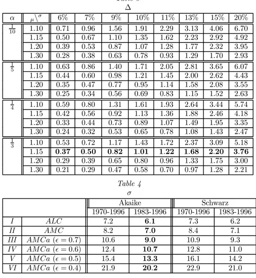
I proceed to calculate ∆, the proportional increase in consumption (or de-crease in the work effort) made possible by the imaginary money scheme. The results are reported in Table 3, again as percentages. All those calculations are based onλ= 1, which would be the optimal monetary policy if monetary frictions vanished from the economy. In the cashless limit, towards which ad-vanced economies are supposedly headed, there would be (in this model) no reason why monetary policy should target anything except price misalignment, and the imaginary money scheme would have its best shot at producing welfare gains.14
14Since∆is simply proportional toθ, results for different values ofλcan be readily
Results are reported for four calibrations of theflex-price mark-up: µ= 1.1, 1.15,1.2and1.3. In the wake of a systematic effort to refine estimates of industry mark-ups spurred by Hall (1988), values in that range have become standard in the calibration of macroeconomic models. Rotemberg and Woodford (1996), for instance, useµ= 1.2. Perhaps more telling, Rotemberg and Woodford (1997, 1999a)findµ= 1.15when they estimate a (partially calibrated) dynamic general equilibrium model with sticky prices intended for the evaluation of monetary policy rules, and I shall focus on that particular value. King and Wolman (1999) calibrate their model withµ= 1.33, an admittedly ‘extreme assumption’ made to exaggerate the distortions associated with market power. As mentioned above, higher mark-ups correspond to lower elasticities of substitution, which mitigate the misallocation of production arising from a given degree of price misalignment.
In dynamic models with staggered prices, calibration ofαis typically based on the implied mean duration of prices. Rotemberg and Woodford (1997, 1999a), for instance, calibrate their quarterly model to match a mean dura-tion of prices of three quarters, as found by Blinder (1994) and Blinder et al. (1998). Such calibration of a quarterly model would imply that only a third of the prices change before one semester of being set, which is also approximately in line with thefinding of Blinder et al. that 35% offirms do adjust prices that often. All that suggests interpreting the length of the period described in my model as one semester, and settingα= 1
3. Table 3 reports results for lower α’s
as well, on the grounds that a shorter periodicity for parity changes - and, thus, for the model as a whole - would not be inconceivable, in order to operate at a horizon over which price stickiness is indeed more pronounced. Note that it is important that bothσandαbe measured for the same frequency.
The main difficulty in the calibration is tofind reliable numbers for σ. Let
d
MC(z)be the percentage deviation of industryz’s nominal marginal cost from its expected value, and denote by MCd the mean of these deviations across all industries. Then,MCd(z) =bs(z) +Pb+wb andM Cd =bs+Pb+wb. For industry
z, the standard deviation of the idiosyncratic shocksb(z)−bscan also be written as:
σ(z) = r
varhMCd(z)−MCdi
In the model, those are the same for every industry, an assumption that is unlikely to hold in the data. Short of incorporating heteroskedasticity into the model (thereby ruining its symmetry), a natural solution is to calibrate its generic variance according to a cross-sectional weighted average of all esti-mated sectoral variances. But the estimation of eachσ(z)is complicated,first of all, by the unobservability of marginal costs - which, unlike in the model, need not coincide with average variable costs. Even after a suitable proxy for marginal costs is found, there remains the unobservability of their one period ahead forecasts and the respective unforecasted residuals.
Table 4 displays some (still crude) estimates, expressed as percentages. These estimates are described in detail in the next section, where I argue that rowsIIIandIV should be regarded as containing reasonably conservative esti-mates ofσ, which depend however on a number of assumptions and on further estimates of key technology parameters. Calibrated differently, but still quite plausibly, the same method produces the higher values of row V, while those in rowV I are probably best interpreted as outside figures forσ. Rows I and
II are almost certainly underestimates, presented as a loose but robust lower bound. The columns differ with respect to how the one period ahead forecasts of marginal costs are constructed, and with respect to the time period covered by the calculation - either including or excluding the large relative price changes prompted by the oil shocks. I focus on the second column, which produces the most conservative estimates ofσ. All those numbers are estimated from yearly data, and it is unclear how they should be adjusted to go along with anα cal-ibrated for higher frequencies: the adjustment could actually could go either way, depending on the serial correlation of the cost shocks within the year, on which I have no information.
Ifσ belongs to the 9-11% range suggested by rowsIII andIV, then gains from imaginary money of about 0.8-1.2% of output should be expected under the benchmark calibration (that is, forµ= 1.15andα= 13). At the 6-7% lower bound for σ shown in rowsI and II, the efficiency gains should fall between 0.4% and 0.5% of output. Gains would amount to 1.7% of output forσ= 13% (the value in row V), rise to 2.2% when σ = 15%, and reach 3.8% if σ were indeed 20% as rowV I indicates.
Numbers of that order sound substantial when compared to the gains one presumes improved macroeconomic stabilization capable of delivering. Unlike tuning the parameters of a monetary policy rule, however, they come at a cost - the calculation burden of the multiple units of account. The magnitude of the latter is extremely hard to get a handle on. There are published estimates of currencyexchange costs (the costs of transacting in foreign exchange markets): the EMU expected to save between 0.3% and 0.4% of GDP in that rubric, according to Emerson et al. (1992). But those arenot the costs that imaginary monies would entail, if the means of payment were kept unique. It is also clear that calculation costs proper - the nuisance of converting prices from one unit of account to another for purposes of comparison and settlement - would be much more widespread in a non-locational imaginary money scheme than in a world with multiple national currencies, where they remain circumscribed to cross-border transactions. There seems to be little hope of putting a value on that nuisance except by introspection.15
15In another model-based welfare analysis, Canzoneri and Rogers (1990)find that Europe
3.4
Estimating
σ
The estimates ofσcontained in Table 4 are based on US data from the Man-ufacturing Industry Database, maintained by Eric J. Bartelsman, Randy A. Becker and Wayne B. Gray under the auspices of the NBER and the US Cen-sus Bureau. The database and its documentation (Bartelsman and Gray, 1987) can be downloaded from the NBER website.16 It contains yearly cost and out-put information for the 458 manufacturing industries of the 1987 4-digit SIC classification, for the period 1958-1996.17
The estimates ofσrely on the following variables: V SHIP (the dollar value of sales),IN V EN T (the value of end-of-year inventories),P RODW (nominal wage bill for production workers), M AT COST (nominal outlays on materi-als and energy), P ISHIP (an implicit deflator for the industry’s sales), and
P IMAT (an implicit deflator for the industry’s outlays on materials and en-ergy). Those are used to construct industry series (1959-1996) for nominal average costs of intermediate inputs and production labor, defined as:18
ALCt(z)≡
P RODWt(z)
V SHIPt(z)+INV ENTt(z)−INV ENTt−1(z) P ISHIPt(z)
AM Ct(z)≡
M AT COSTt(z)
V SHIPt(z)+INV ENTt(z)−INV ENTt−1(z) P ISHIPt(z)
If the production function is isoelastic in production labor, thenALCt(z)will be a constant multiple ofM Ct(z)(see Bils, 1987, or Rotemberg and Woodford, 1999b), and thus ALC[t(z) =M Cdt(z). Likewise, if the production function is isoelastic in intermediate input use, then AMC\t(z) =M Cdt(z). Under these conditions, we would have two candidate proxies for the unobservable marginal costs.19
To get at the cost surprise, I assume that each industry forms univariate forecasts of its own time series of costs, for the period 1970-1996. More precisely, I let each industry ‘choose’ an AR specification forlogALCt(z)−logALCt−1(z),
with any number of lags between 1 and 10, using 1970-1996 as a fixed sample period, and relying on as many data points as necessary from the 1960-1969 pre-sample offirst differences. In order to automate that operation for the 458
disregard the effects associated with sticky prices considered here.
16I am grateful to Randy Becker for kindly and promptly providing me with additional
clarification.
1 7There are actually 459 codes, but I disregard one industry (asbestos) due to its mid-sample
demise.
1 8As Bartelsman and Gray (1987) warn, the adjustment for inventory increases performed
below is not entirely reliable, both because of the quality of the inventory data and because
P ISHIPis a deflator of sales, not production.
19One might be tempted to consider the broaderALC+AM C(the average variable cost) as
series, the choice is based on an easily computable criterion - I report results using Akaike’s Information Criterion and Schwarz’s Criterion. The operation is repeated forAM C.
The estimated AR processes of each industry is used to generate one pe-riod ahead forecasts for the industry levels of ALC and AMC, from 1970 to 1996. Percentage deviations of realized from forecasted values, ALC[t(z) and AM C\t(z), are then calculated. For each year, I calculate cross-sectional averages of these deviations, ALC[t and AM C\t, both weighted according to the participation of each industry in the year’s aggregate output (the sum of
V SHIPt(z)+IN V EN Tt(z)−IN V EN Tt−1(z)over allz). Finally, sample time
series variances ofALC[t(z)−ALC[t andAM C\t(z)−AM C\tare computed for each industry, either over the whole sample (1970-1996) or just over the post-oil shock half-sample (1983-1996). The industry-specific variances are then aver-aged, with weights given by the output participation of each industry in the mid-sample year of 1983. Theσ’s reported in rows IandII of Table 4 are the square root of those results.
The problem is that neitherAM LnorAM Cis likely to be a very good proxy for marginal costs, because there is strong evidence that production functions are isoelastic neither in production workers nor in intermediate inputs.20 In reality, different factors are believed to be less substitutable in the short run than in the common long run Cobb-Douglas specification of production technology. As a result, bothALC andAM C would require corrections in order to proxy well for marginal costs. In their raw state, these variables would actually vary less than marginal costs; inasmuch as muted volatility makes them easier to forecast, they would tend to impart a downward bias toσ.
WithALC, the problem is compounded by a number of nagging measure-ment issues that should be much less serious regardingAMC. In order to avoid those additional difficulties, I work withAM C, using the procedure described in Rotemberg and Woodford (1999b) to calculate the adjusted series:
AM Cat(z) = exp [logAMCt(z)+
1−sM(z)
sM(z)
¡
1−1²¢ ³1−µsM(1 z)´logP IMATAMCt(t(z)z)i (25)
where µ is the mark-up, sM(z) is the industry’s average share of intermedi-ate inputs (mintermedi-aterials and energy) in the value of output, ² is the elasticity of substitution between intermediate inputs and primary factors, and P IMATAMCt(t(z)z) measures the intermediate inputs to output ratio.21 When²= 1, no adjustment
20On this question of the biases ofALC and AM C as proxies for marginal costs, I draw
heavily on Rotemberg and Woodford (1999b).
2 1The procedure is described by Rotemberg and Woodford (1999b, pp. 1064-5), and relies
is required, andAM Cis indeed (up to afirst order approximation) a good proxy for marginal costs.
For each industry, sM(z) can be calculated as the time series mean of AMCt(z)
P ISHIPt(z). The mark-up is set at µ = 1.15, the benchmark calibration of
last section, and applied across the board to all industries in the sample. The elasticity of substitution is also assumed common to all industries; I calibrate it first at ² = 0.7, which is approximately the value estimated by Rotemberg and Woodford (1996). That estimate is obtained from industry data at the 2-digit SIC level, and some of the measured substitution between intermediate inputs and primary factors might be picking up substitution across products that, within the same 2-digit code, happen to be more intensive in one or the other. Within each 4-digit industry code considered here, there should be fewer such opportunities to substitute across products, and one might expect a lower
²when estimated at that finer level of disaggregation. Lower estimates would also be expected if, unlike Rotemberg and Woodford, one measured factor sub-stitution within the year instead of that happening over two year horizons. In order to account for that fact, and to indicate the sensitivity of the results to lower elasticities, I make the same calculations using²= 0.6, 0.5and0.4.
RowsIII toV I of Table 4 contain the corresponding values of σ, obtained by running the adjustedAM Caseries through the same steps described above forALC and AMC. The only difference is that I truncate the cross-sectional distribution of industry-specific variances, in order to weed out spurious out-liers before calculating the averageσ2. The problem is that, as the elasticity of substitution ² falls towards zero, less substitutability should be reflected in less variability in the intermediate inputs to output ratio, or else the adjust-ment term in (25) would start displaying wild swings. When I apply a lower elasticity of substitution across the board, such wild swings start showing up in some industries, producing extremely high variances for their idiosyncratic shock surprises - high enough to noticeably inflate the cross-sectional average of these variances. Inspection of the cross-sectional distributions of variances re-veals that discarding the eight highest (among the 458) takes care of the outlier problem in every case considered in Table 4. So, the results in rowsIII toV I
consider only the 450 lowest variances in each case.22
Restricting attention to univariate techniques could be faulted for not giving a chance to all potential regressors available in the database, and thus produc-ing inefficient forecasts. But univariate techniques are not atypical in industry projections, and it would seem particularly artificial to assume that each indus-try can use cost data of any other indusindus-try. But forecasts might be improved if the regressions were allowed to include a practicable amount of additional in-formation, including macroeconomic data as well as price and (perhaps lagged) cost data for closely related sectors. Even if real world industry participants
22Even if there were genuine outliers in the sample, one could make a case for excluding
do not forecast much better than implied by the univariate projections above, normative implications for imaginary monies should not rely on gains that could be more easily obtained through a general improvement in forecasting ability. On the other hand, it would be more plausible to use real time estimates of the process for marginal costs, on which out-of-sample projections would be based. In closing, it should be noted that estimates ofσbased on the 458-strong list of industries of the 4-digit SIC might still suffer from a significant downward aggregation bias. That level of disaggregation might still be averaging out a considerable amount of variation across differentiated products included in the same 4-digit category. It also averages away allspatial variation in cost shocks - for non-tradeables, that variation should also be matched by movements in relative prices.
4
Conclusion
Disembodied units of account have reappeared a number of times since the me-dieval and early modern occurrences mentioned in the introduction. In none of those, however, did they share the spirit of the imaginary money scheme exam-ined in this paper. The euro, yet to become a circulating medium of exchange, has afixed parity with respect to all circulating currencies that joined the EMU. Parities were not so irrevocablyfixed in the case of its virtual predecessor, the ECU, but that one was not in widespread use as a pricing unit (Bordo and Schwartz, 1989). Some high inflation economies managed to contain outright currency substitution by instituting indexed units of account. But their use in pricing was not meant to facilitate relative price changes prompted by idiosyn-cratic supply or demand shocks; quite to the contrary, the goal was to avoid undue relative price changes associated with staggered price adjustments under persistent inflation.23
The fact that the scheme is nowhere to be seen might be construed asprima facie evidence that it has little to offer - otherwise, it should have somehow come into existence. I do not share this view, nor the view that the scheme is bound to be produced by market forces as soon as the economy is ripe for it - say, after technology reduces calculation costs further. Impediments to such spontaneous generation include classic coordination failures and possible conflicts with antitrust regulation. If imaginary monies will ever stand a chance, that may well involve a public policy initiative to publicize the alternative units of account and to manage their parities.
Market forces, however, can be entrusted with the partition of price setters across units of account, once those are in place. If monetary and parity policies target price misalignment alone, then the economy will voluntarily partition itself exactly as a central planner would have dictated. Whoever believes in gains from exchange rateflexibility within a certain region should expect from imaginary monies gains at least as large, if not larger, now that the economy will
23The case of Chile is particularly interesting in that the indexed unit of account, theunidad
optimize overall partitions of price setters, including candidates not beholden to territorial lines.
As long as monetary frictions remain important, it is natural for monetary policy to worry more about price stability in real money than in imaginary monies. The latter, being exposed to larger fluctuations in purchasing power than the former, will be relatively disadvantaged as pricing units. Price mis-alignment will then be mitigated to a lesser extent - to a much lesser extent, actually, if a stable price level in real money is the overriding objective of mon-etary policy. Imaginary monies are unlikely to be attractive if monmon-etary policy is not willing to play along to some extent.
Favoring a stable price level in real money at the expense of stability in imaginary money prices may even introduce an externality in the choice of unit of account. Imaginary monies might be not only less used than the real money, but also less used than would be socially optimal, given the monetary and parity policies. But the impact of that externality on price misalignment is minor, detracting little from the effectiveness of the imaginary money scheme.
In a simple model calibrated after the US economy, the likely gains fromone imaginary money would be somewhere in the range of 1% to 2% of aggregate output. That leaves untapped some upside potential for the size of the gains: they might be even larger at higher frequencies, or if the variance of idiosyn-cratic shocks to marginal costs were estimated at afiner level of disaggregation. Moreover, that amounts to 40.5% of the deadweight loss from price stickiness, and one could go after the remainder armed with additional imaginary monies. Whether gains of that magnitude - or of any plausible magnitude - are enough to compensate for the nuisance of calculating price conversions is a question likely to remain open.
If there is little hope of settling the question of how large that calculation burden would be, much progress can still be made in assessing the potential gains from imaginary monies. First, the estimation in section 3.4 could be refined in several self-evident dimensions. Second, my theoretical model is a convenient exposition vehicle, but it is too rudimentary as a laboratory economy on which to test normative implications for the real world, particularly along the following dimensions:
1. Lack of dynamics: In a dynamic model with forward looking price setters, it would no longer be true that only idiosyncratic surprises to marginal costs matter. Expected future shocks would also generate price misalign-ment, as producers set their current prices preventively. Moreover, with staggered price adjustments, one would expect more protracted misalign-ment to be associated with the same mean duration of prices.
specification also implies a correlation matrix with constant entries along every diagonal, a neat but unlikely pattern that facilitates the design of an effective menu of imaginary monies.
3. Marginal cost curves: If marginal cost curves are truly upward sloping, the assumption that they are instead flat leads the model to overstate the deadweight loss from price stickiness associated with any empirically measured variance of marginal costs. That applies to measured variance due both to shocks that shift cost curves and to shocks that shift demand curves along the same upward sloping marginal cost curve. When sectoral output is below equilibrium, the deadweight loss is overstated because the model assumes that the shortfall could be produced at the low realized marginal cost. When output exceeds equilibrium, the overstatement is due to counting every inframarginal unit as if it had been produced at the high realized marginal cost.
4. Policy implementation: The model assumes that policymakers directly observe cost shocks all around the economy, before deciding on the settings of monetary and parity policies. In reality, they would have to rely on indirect evidence of cost shocks, such as relative price movements already observed. Policies described by reaction functions to realistic information sets would be more limited in their ability to mitigate price misalignment.
As they stand, the results suggest that multiple units of account linked by managed parities are not a policy instrument to be simply dismissed out of hand. Needless to say, they do not suffice to trigger a rush to experimentalism with monetary architecture, especially in the light of the caveats just listed. But they are hopefully enough to whet the appetite for more ambitious quantitative work on the subject.
References
[1] Ball, Laurence and N. Gregory Mankiw, “Relative-price changes as aggre-gate supply shocks”,Quarterly Journal of Economics 110: 161-93, 1995.
[2] Bartelsman, Eric J. and Wayne Gray, “The NBER Manufacturing Produc-tivity Database”, NBER Technical Working Paper 205, 1996.
[3] Bils, Mark, “The cyclical behavior of marginal cost and price”,American Economic Review 77: 838-857, 1987.
[4] Blinder, Alan S., “On sticky prices: Academic theories meet the real world”, in N. Gregory Mankiw (ed.),Monetary Policy, University of Chicago Press, 1994.