t
I
I
I
,
•
•
••
•
Seminário de Pesquisas Econômicas
•
•
•
•
•
•
•
•
•
•
•
•
•
•
•
•
•
•
•
•
•
•
•
•
•
•
•
•
A
Month!y Indicator of
Brazilian
GDP
Professora Marcelle Chauvet
(University of California)
Data: 07/12/00 (quinta-feira)
•
Realização:
:
,.
•
•
•
•
•
•
•
•
FUNDAÇÃO
GETUUO VARGAS
EPGE
Escola de P6s-GracUlção
em Economia
Informações:
Praia de Botafogo, 190 - 10
0andar - Auditório Eugênio Gudin
22253-900 Rio de Janeiro - RJ
Brasil
Tel.: (21) 559-5834
•
•
•
•
•
•
•
•
•
•
•
•
•
•
•
•
•
•
•
•
•
•
•
•
•
•
•
•
•
•
•
•
•
•
•
•
•
•
•
•
•
•
•
•
•
•
•
•
•
A MONTHLY INDICATOR OF BRAZILIAN GDP
September 2000
Abstract
This paper constructs an indicator of Brazilian GDP at the monthly ftequency. The peculiar instability and abrupt changes of regimes in the dynamic behavior of the Brazilian business cycle were explicitly modeled within nonlinear ftameworks. In particular, a Markov switching dynarnic factor model was used to combine several macroeconomic variables that display simultaneous comovements with aggregate economic activity. The model generates as output a monthly indicator of the Brazilian GDP and real time probabilities of the current phase of the Brazilian business cycle. The monthly indicator shows a remarkable historical conformity with cyclical movements of GDP. In addition, the estimated filtered probabilities predict
ali recessions in sample and out-of-sample. The ability of the indicator in linear forecasting growth rates of GDP is also examined. The estimated indicator displays a better in-sample and out-of-sample predictive performance in forecasting growth rates of real GDP, compared to a linear autoregressive model for GDP. These results suggest that the estimated monthly indicator can be used to forecast GDP and to monitor the state of the Brazilian economy in real time.
KEY WORDS: Business Cycle, Dynamic Factor, Markov Switching,
Composite Indicators, Kalman filter, Filtered Probabilities, Forecast.
JEL Classification Code: C32, CSO, E32
r Department ofEconomics, University ofCalifornia, Riverside, CA 92521-0247; phone: (909) 787-5037 x1587; fax: (909) 787-5685.
•
•
•
•
•
•
•
•
•
•
•
•
•
•
•
•
•
•
•
•
•
•
•
•
•
•
•
•
•
•
•
•
•
•
•
•
•
•
•
•
•
•
•
•
•
•
•
•
•
1. Introduction
In recent years, reduction in capital restrictions in emerging markets substantially
increased international financial flows to these countries. In Brazil, the stability of the
currency post-Real plan set the basis for reforms, which tumed Brazilian markets more
competitive. Trade liberalization and a stronger currency led to cheaper imports and
propelled national fmns to modernize their technology. These changes combined with
privatization and deregulation of state monopolies attracted record high foreign investrnents.
The economic reforms, however, have not decreased the entrenched volatility of the
Brazilian economy. Abrupt downturns and upturns have been a regularity affecting both
financiaI markets and the goods producing sector. As international markets become more
integrated, there has been a surging interest in the overall economic performance of Brazil. In
particular, there has been an increasing international demand for timely and reliable data that
would al10w real time assessment of the dynamics of the Brazilian economy. The availability
of more accurate real time inforrnation about the Brazilian economy is not only important for
policy or investment decisions. It can also contribute to make it less likely the occurrence of
self-fulfilling financial crisis driven by misperceptions regarding fundamentals ofthe Brazilian
economy and the country risk.
A traditional method of monitoring the economic activity is through the use of
composite leading and coincident indicators. In the U.S., composite indicators have been
used since their first construction by the Department of Commerce in the 1960s,1 based on
the work of Burns and Mitchell (1946). As a result of a throughout statistical analysis of
macroeconomic variables, Burns and Mitchell classified over 500 series into lagging,
coincident, or leading according to the timing of their cyclical movements with the U.S.
economic activity, in a research sponsored by the National Bureau of Economic Research
(NBER). The combination of some of these variables resulted in the composite indexes,
which are used to signal turning points of business cycles.2 These indicators are one of the
most watched series by the press, businesses, policymakers, and stock market participants.
1 Since 1995 tbe Conference Board has been responsible for compiling tbe U.S. composite indicators.
2 Tuming points refer to peaks and troughs of business cyc1e phases. Peaks mark the beginning of recession phases (end of expansions) and troughs define the end of recessions (onset of expansions).
•
•
•
•
•
•
•
•
•
•
•
•
•
•
•
•
•
•
•
•
•
•
•
•
•
•
•
•
•
•
•
•
•
•
•
•
•
•
•
•
•
•
•
•
•
•
•
•
•
The popularity of the V.S. economic indicators led to the construction of these
indexes for other countries, such as Australia, Japan, Canada, and other members of the
OECD in the 1970s and 1980s. More recently, progressive market integration has induced a
worldwide interest in the analysis of cyclical fluctuations through the use of economic
indicators. This has placed the traditional method to construct the indicators in the spotlight,
which has been under increased scrutiny and criticism in recent years.3 One of the main
criticisms is as old as the method itself. Koopmans (1947) criticized Burns and Mitchell's
analysis for being centered on measurement without any explicit model attached to it. This
problem is also extended to composite indicators, whic h are constructed as simple weighted
averages of statistical transformations of their components. This implies that the dynamic
relationships among the variables are not taken into account. For example, the method
ignores their cross-correlations or potentiallong-term relationships. Another criticism is that
the method does not include a probabilistic model to determine turning points in the
indicators, and the existing ad-hoc rules require the use of substantial ex-post data. That is,
turning points can only be identified and predicted a couple of months after their occurrence,
which undermines the usefulness of indicators for real time forecasting. Finally, large
revisions have been implemented in the indicators over the years to improve their ability in
predicting turning points ex-posto These revisions, which include changes in the
components, in their weights, and in the construction procedures, have substantially changed
the historical record of the indicators' performance. In fact, analysis of their real time
forecasting ability can only be evaluated using the unrevised versions of the indicators, as
examined in Diebold and Rudebusch (1991).4
The disseminated use of economic indicators and awareness of their shortcomings
had a corresponding resurgent academic interest in this instrumento Frontier econometric
models have been used to formally explore potential dynamic differences across business
cyc1e phases, to generate indicators, and to determine turning points.
3 Boldin (1998/1997) summarizes the main criticisms to the composite indicators.
4 Following Diebold and Rudebusch (1991), severa! other authors bave examined the reliability of the
umevised leading indicator in predicting tuming points in real time, such as Emerson and Hendry (1996),
Lahiri and Wang (1994), perez-Quiros and Hamilton (1996), Chauvet (1998/1999), among others.
•
•
•
•
•
•
•
•
•
•
•
•
•
•
•
•
•
•
•
•
•
•
•
•
•
•
•
•
•
•
•
•
•
•
•
•
•
•
•
•
•
•
•
•
•
•
•
•
•
The goal of this paper is to cbtain an indicator of Brazilian GDP at the monthly
frequency that can be used to forecast business cycles and to monitor the current state of
the economy in real time. In particular, a Markov switching dynarnic factor model is used to
combine several macroeconomic variables that display simultaneous comovements with
aggregate economic activity, as in Chauvet (1998). The model generates as output a
monthly indicator of the Brazilian GDP and real time probabilities of the current phase of the
Brazilian business cycle.
The formal representation of business cycle phases through the dynamic factor
model with Markov switching overcomes the drawbacks of the traditional method while
maintaining the main points of Burns and Mitchell (1946) and the NBER's definition of
business cycles, as suggested by Diebold and Rudebusch (1996). First, since the model
includes several variables, it captures pervasive cyclical fluctuations in various sectors of the
economic activity. As recessions and expansions are caused by different shocks over time,
the inclusion of different variables increases the ability of the model in representing and
signaling phases of the business cycles. In addition, the combination of variables reduces
measurement errors in the individual series and, consequently, the likelihood of false signaling
turning points, which is particularly important for monthly data. For example, one of the
findings is that the individual variables that compose the indicator, specially industrial
production, do not represent broad changes in the economy and, by itself, give several false
turning point signals. Finally, the model alIows potential asymmetries across expansions and
recessions and analysis of turning points, albeit here their evaluation can be followed in real
time.
In order to compile a composite indicator as accurately as possible, a large number
of economic time series were evaluated in-depth, with special attention to the peculiar
dynarnical behavior of the Brazilian business cycle. In particular, the instability and abrupt changes of regimes in the history of Brazilian economic activity were explicitly modeled
within nonlinear frameworks.
The primary step in developing composite indicators is the definition of a business
cycle chronology to be used as a benchmark. That is, it is necessary to first determine peaks
and troughs of the Brazilian business cycle, which are then used to evaluate the predictive
performance of the indicators. The NBER has been dating the U.S. business cycle for the
•
•
•
•
•
•
•
•
•
•
•
•
•
•
•
•
•
•
•
•
•
•
•
•
•
•
•
•
•
•
•
•
•
•
•
•
•
•
•
•
•
•
•
•
•
•
•
,
,
last fifty years. Peaks and troughs are detennined from a subjective consensus among the
ten members of the Business Cycle Dating Committee. Decisions about business cycle
tuming points are based on the tuming points of several coincident variables, such as
manufacturing and trade sales, personal income, industrial production, and non-agricultural
employment, among others. However, the NBER dating can not be used to monitor the
economy in real time, since the Business Cycle Committee meets only months after a tuming
point has occurred.
In this paper, the results of the monthly indicator of GDP are compared to the
business cycle chronology obtained in Chauvet (2000). Chauvet uses a model-based
approach to date the Brazilian business cycle and growth cycle in the last 100 years.5 The
results are compared with several ad-hoc mIes, and the dating obtained is very similar.
However, the ad-hoc rules require that a couple of months have passed for the tuming point
dating to be detennined. On the other hand, the results of the model-approach method enable
analysis of business cycles on a current basis.
The monthly indicator of Brazilian GDP includes variables measuring aggregate
economic activity such as employment, industrial production, capacity utilization,
compensated hours, and real wages. The estirnated indicator shows a remarkable historical
conformity with cyclical movements of GDP with respect to volatility, timing of peaks and
troughs, and duration of the phases. In addition, the estimated filtered probabilities predict all
recessions and expansions in the sample, as dated in Chauvet (2000).
The performance of the indicator is also examined out-of-sample. In order to
emulate forecasting in real time, the model is recursively re-estimated out-of-sample. This
allows u; to reproduce the information content that was available to forecasters at any point
in time. The indicator summarizes information in several macroeconomic variables, which is
found to be relevant in forecasting economic activity. In particular, the resulting filtered
probabilities predict all recessions out-of-sample. The ability of the indicator in linear
forecasting growth rates of GDP is also examined within and out-of-sample. In both cases
the estirnated indicator displays a better predictive performance compared to a linear
5 More specifica1ly, a MarIrov switching mede! is fitted to quarterly and annual real GDP, and the resulting smoothed probabilities are used as filtering roles to determine tuming points.
•
•
•
•
•
•
•
•
•
•
•
•
•
•
•
•
•
•
•
•
•
•
•
•
•
•
•
•
•
•
•
•
•
•
•
•
•
•
•
•
•
•
•
•
•
•
•
•
•
autoregressive model for GDP. In particular, the inclusion of lags of the indicator improves
substantially forecasts of the severity of recessions and strength of expansions, as measured
by the volatility of changes in GDP.
The results suggest that the indicator and the associated probabilities of business
cycle phases could be useful tools to forecast GDP and to monitor the state of the Brazilian
business cycle in real time.
The paper is organized as follows. The next section describes the procedure used to
analyze and select the variables that compose the model. Section 3 presents the model. In
the fourth section, the empirical results are discussed. In particular, the probabilities of
business cycle phases and the indicator of the Brazilian GDP are examined within and
out-of-sample. The fifth section concludes.
2. Data Analysis
In order to compile the composite indicator, a large number of economic time series
were considered. The data were obtained from Getúlio Vargas Foundation (FGV) and the
Central Bank of Brazil databases. In order to obtain a historical representative composite
indicator of the Brazilian GDP, an important criterion for selecting the series was their
sample size. Although there are many candidate variables whose cyclical variation could
potentially coincide with the real Brazilian GDP, only a small subset ofmonthly series have a
longer sample going back to the 1970s and 1980s.6
As a starting point for the analysis, the variables were seasonally adjusted using the
X-lI additive method from the V.S. Bureau of the Census. Variables expressed in nominal
terms were deflated using the Global Price Index, IGP-DI, or the Broad Consumer Price
Index, IPCA. 7 Finally, alI variables were transformed to achieve stationarity.8
SeveraI selection criteria were then implemented to find the ones that display
simultaneous movements with the Brazilian business cycles. The underlying guideline was
6 In facto most series start in the 199Os. Those were not selected, since a decade of observations would not be
representative of the bistorical behavior of recessions and expansions in Brazil.
7 Since the Broad Consumer Price Index is onlyavailable from 1979 on, the IGP-DI was utilized for data with langer sample.
•
•
•
•
•
•
•
•
•
•
•
•
•
•
•
•
•
•
•
•
•
•
•
•
•
•
•
•
•
•
•
•
•
•
•
•
•
•
•
•
•
•
•
•
•
•
•
•
•
the economic significance of the series, their statistical adequacy, their 1iming at turning
points, and their overall conformity to the business cycle. First, the series were classified as
coincident, leading or lagging according to their ability to Granger-cause changes in GDP,9
their cross-correlation with changes in GDP in time domain, and coherence in frequency
domain. Second, they were ranked according to the timing of their turning points with
cyclical variation in GDP, which is taken as the reference cycle. Peaks and troughs of GDP
mark recession and expansion phases in Brazil, and were obtained as in Chauvet (2000). In
particular, two-state Markov switching models were fitted to each of the candidate variables
and to GDP, with the states representing economic expansions or contractions.lO The
estimated probabilities of COJltractions were then used to determine peaks and troughs in the
series, and the timing of change of each series was then compared to GDP turning points.
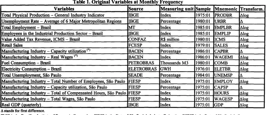
From these procedures, fifteen variables were found to display coincident
movements with changes in CDP, which are described in Table 1. These series represent
different measurements of industrial production, capacity utilization, real wages,
compensated hours, retail sales, employment, unemployment rate, fuel consumption, and
production of cement.
8 During the period analyzed there were severa1 stabilization plans that engendered structmal breaks in the Brazilian macroeconomic variables. Thus, both the augmented Dickey-Fuller (1979) and Perron's (1989) tests were used to verify the hypothesis of unit roots.
9 For comparison with growth rates of GDP, two procedures were undertaken. First, all monthly series were converted to quarterly frequencies as simple averages. Second, changes in GDP were converted into monthly frequency using quadratic-match average for comparison with the monthly series.
10 The best two-state specification for each series was selected based on the likelihood ratio testo
•••••••••••••••••••••••••••••••••••••••••••••••••
Table
1.
Ori2inal Variabl, MonthlvFVariables Source Measurine unit Sample Mnemonic Transform.
Total Physical Production - General Industry Indicator IBGE Index 1975:01 PRODBR ~log
Unemployment Rate - Average of 6 Major Metropolitan Regions IBGE Percentage 1980:01 URBR ~
Total Empl()Yll1ent - Brazil MT Index 1985:01 EMPLBR ~log
Employees in the Industrial Production Sector - Brazil IBGE Index 1985:01 EMPLIP ~log
Value Added Tax Revenue, ICMS - Brazil CONFAZ R$ million 1980:01 ICMS ~Iog
Retail Sales FCESP Index 1979:01 SALES ~Iog
Manufacturing Industrv - Capacity utilization (0) BACEN Percentage 1986:01 CAPBR ~
Manufacturing Industrv - Real Wages (0) BACEN lndex 1986:01 WAGEMI ~Iog
Fuel Consumption - Brazil PETROBRAS Thousands M3 1980:01 COMB ~Iog
Electricity Consumption - Brazil ELETROBRAS GWH 1976:01 ELETBR ~Iog
Total Unemployment, São Paulo SEADE Percentag;e 1984:01 UNEMSP ~
Manufacturing Industrv - Total Number of Em~loxees, São Paulo FIESP lndex 1975:01 EMPLOY ~log
Manufacturing Industrv - Capacity utilization São Paulo FIESP Percenta~e 1975:01 CAPSP ~
Manufacturing Industrv - Total of Compensated Hours São Paulo FIESP lndex 1975:01 HOURS ~Iog
Manufacturin~ lndustry - Total WaAes,- São Paulo FIESP lndex 1975:01 WAGESP ~Iog
Real GDP{quarterlyt mGE lndex 1975:01 GDP ~Iog
.ó. stands for first difference.
mGE is the Brazilian lnstitute of Economic Geography. FIESP is the State of São Paulo's IndustIY Federation. FCESP is the State of São Paulo's Commerce Federation. MT is the Labor Ministry. CONFAZ is the National Treasury Council. BACEN is the Central Bank of Brazil. SEADE is State of São Paulo System ofData Analysis. ELETROBRAS is the Brazilian Electricity Holding Company. PETROBRAS is the Brazilian Petroleum Holding Company.
(.) These data were generated from surveys ofthe Industry Federation in the following Brazilian States: Amazonas, Ceará, Pernambuco, Bahia, Esplrito Santo, Minas Gerais, Rio de Janeiro, São Paulo, Paraná, Santa Catarina, Rio Grande do Sul e Goiás.
7
•
•
•
•
•
•
•
•
•
•
•
•
•
•
•
•
•
•
•
•
•
•
•
•
•
•
•
•
•
•
•
•
•
•
•
•
•
•
•
•
•
•
•
•
•
s
,
,
•
3. The Model
The indicator of the Brazilian business cycle is constructed using a Markov
switching dynamic factor model, as in Chauvet (1998). Let 1'; be a vector ofnxl observable
macroeconomic variables that move simultaneously with the Brazilian Gross Domestic
Product:
(1)
Changes in these n macroeconomic variables ~ Yt are modeled as a common unobserved
scale factor, ~F" and n individual idiosyncratic terms, ~Vt. The factor loadings, Â., measure
the sensitivity of the series to the dynamic factor, Mt. 11 Both the factor and the idiosyncratic
terms follow autoregressive processes:
(2) TIs, -N(O, cr~,
),
(3) Et - i.i.d. N(O, l:).
where TIs, is the common shock that engender changes in the phases of the business cycle
and Et are the measurement errors. In order to capture potential asymmetries across
different states of the business cycle, the intercept and variance of the factor switch regimes
according to a Markov variable, S" where ~ = (l1+(lOS" and
S
= 0, 1. That is, theeconomy can be either in an expansion state (St= 1 ), where J.Ls. is positive; or in a
contraction phase (St=O), with a negative mean growth rate. The volatility of the factor as
measured by cr~ can also assume different values across states. The switches from one
state to another is determined by the transition probabilities of the first-order 1wo-state
Markov process, Pij=Prob[SdISt_I=i], where
LJ~~P
..
= 1,~j
= 0,1.IJ
The model separates out common signal underlying the observed variables from
individual variations in each sector of the economic activity. The dynamic factor captures
widespread simultaneous downtums and upturns movements of several sectors of the
11 The factor loading for lhe production series is set equal to one to provide a scale for the latent dynamic factor. This normalization is a necessary condition for identification of the factor and the choice of parameter scale does affect any of the time series properties of the dynamic factor or the correlation with its components.
•
•
•
•
•
•
•
•
•
•
•
•
•
•
•
•
•
•
•
•
•
•
•
•
•
•
c.
•
•
•
•
•
•
•
•
•
•
•
•
•
•
•
•
•
•
•
"
"
•
Brazilian economy, corresponding to Bums and Mitchell's (1946) definition of business
cycles. On the other hand, if only one of the variables falls (e.g. industrial production), this
would not characterize a recession in the model, and it would be captured by the industrial
production idiosyncratic termo A recession (expansion) will occur when alI n variables
decrease (increase) at about the same time. That is, lls
t and ~Vt are assumed to be mutually
independent at alI leads and lags, for alI n variables, and d(L) is diagonal.
The dynarnic factor is the outcome of averaging out the discrete states. Although the
n variables measure economic activity in specific sectors, the dynamic factor is a nonlinear
combination of them, representing broader movements in the Brazilian economy. The
estimation procedure is discussed in the Appendix.
4. Empirical Results
Given that the sample availability differs across variables, the model was estimated
using three periods: a) from 1975:01 to 2000:06, b) from 1980:01 to 2000:06, and c) from
1986:01 to 2000:06. Six variables are available from 1975:01 00, which are used to estimate
the indicator with the longest período For 1he second sample, these variables are combined
with the other four that start in 1980:01. Fina1ly, these ten variables are combined with the
remaining five to estimate the composite indicator from 1986:01 on.
The dynamic factor summarizes the comovements underlying the macroeconomic
series used in the model. Thus, it is crucial that the variables composing the indicator display
coincident cyclical movements with each other.J2 Factor ana1ysis and principal components
were used to test the variables to be included in the factor. The magnitude ofthe eigenvalues
of the common factor's correlation matrix indicates whether the factor structure is a
reasonable representation of the data. In fact, this method can also be used to test for single
or multi-factor specifications.
Finally, the selection among those that represent closely related definitions was
based on two guidelines. First, it was taken into consideration the economic significance of
the specific activity or process as more representative of the Brazilian GDP. For example,
12 The inc1usion of variables with low correlation with each other will genera1ly result in the convergence of the factor to one ofthe component variables.
•
•
•
•
•
•
•
•
•
•
•
•
•
•
•
•
•
•
•
•
•
•
•
•
•
•
•
•
•
•
•
•
•
•
•
•
•
•
•
•
•
•
•
•
•
•
•
•
•
total industrial production is chosen instead of production in the manufacturing industry, and
so on. Second, the evaluation process described in section 2 was applied to rank and select
between closely related variables.
From this analysis, three coincident indicators are found from the combination of a
small set of variables. For the sample from 1975:01 on, tive variables are combined to yield
a monthly indicator of GDP (group 1): total industrial production (PRODBR), total number
of employees (EMPLOY), capacity utilization (CAPSP), compensated hours (HOURS), and
total wages (WAGESP)Y For the sample from 1980:01, six variables were combined to
obtain the indicator (group 2): total industrial production (PRODBR), unemployment rate
(URBR), compensated hours (HOURS), retail sales (SALES), capacity utilization (CAPSP),
and total wages (WAGESP). Finally, for the sample from 1985:01 on, six variables enter
into the composition of the coincident indicator (group 3): total industrial production
(PRODBR), total employment (EMPLBR), compensated hours (HOURS), retail sales
(SALES), capacity utilization (CAPBR), and total wages (W AGEMI).14
The models using the three sets of variables were estimated by maximizing the
likelihood function through a numerical procedure. The nonlinear discrete tilter produces
two outputs: the dynamic factor and the associated probabilities of the Markov state. The
filtered probabilities give at time t the probability of the Markov state using only information
available at t, Pr(SI=O, 1
11
1). On the other hand, the smoothing probabilities are obtainedthrough backward recursion using the information in the full sample, Pr(St=O,llh).
Figure 1 shows the smoothed probabilities of recession for the three sets of
variables. The results are striking similar. The probabilities match in terms of timing of
changes, duration, and amplitude. This also holds for the dynamic factor from the three
models, where the correlation for each pair is around 0.999. This finding is due to the fact
13 Variables measuring electricity usage were found to lag the economic activity. This result might reflect in
part the way some of these series are calculated. For example, observation for time t corresponds to electricity usage from. mid-month t-l to mid-month t The series on fileI consumption exhibits low correlation with most of the other components and was, therefore, not included in the final composite indicator. The value added tax revenue series (ICMS) did not score very high in the evaluation process - in addition to being a very noisy variable, it also displays low correlation with current economic conditions at the monthly frequency, which may be a consequence of measurement error.
14 The hypothesis of cointegration for these three group of series was rejected at the 5% leveI using ]ohansen's (1991,1995) test
•
•
•
•
•
•
•
•
•
•
•
•
•
•
•
..
•
•
•
•
•
•
•
•
•
•
•
•
•
•
•
•
•
•
•
•
•
•
•
•
•
•
•
•
•
•
~
,
"
that the series used in each subset represent the same sectors. Basically, the variables are
broader or narrower measurements of employment, wages, industrial production, capacity
utilization, and sales.15 Thus, the empirical analysis is shown for the monthly indicator
composed of the variables with a longer historical sample, group 1.
Figure 1- Smoothed Probabilities ofRecessions for Group 1 (-), Group 2 (-),
and Group 3 (- - -):
1.0
-
~
1
1~
,
I
-
i
r
,~
I I')
I ~
I
l~
-
I
I
0.8
0.6
0.4
II
11
J
-lAJ~
vwjl
V
I
'Jj
V
t
J
IV
I
~
~
0.2
0.0
76
78
80
82
84
86
88
90
92
94
96
98
4.1 Specification Tests
The model assumes that the factor summarizes the common dynamic correlation
underlying the observable variables, which implies that the n residuaIs áVt are uncorrelated
across variables. This assumption is tested in several ways. First, the one step ahead
forecast errors obtained from the Kalman filter are not predictable by lags of the observable
variables. Second, the disturbances are regressed on six lags of the observable variables, and
the parameters of the equation are not significantly different from zero. These results support
15 Notice that these are rougbly the same variables used by the NBER, the Conference Board, and the OECD to construct their coincident indicators ofthe business cycle. The similarity ofthe results for the three groups
a1so indicate that the series representing the production process in São Paulo are good proxies for the broader production process in the whole country. A further examination ofthe data explains this finding - São Paulo's GDP has corresponded to around 60% ofthe total Brazilian GDP in the last twenty years (data for GDP per
Sate is obtained from mGE).
11
•
•
•
•
•
•
•
•
•
•
•
•
•
•
•
•
•
•
•
•
•
•
•
•
•
•
•
•
•
•
•
•
•
•
•
•
•
•
•
•
•
•
•
•
•
,
,
,
"
the single factor specification, since the idiosyncratic tenns are not capturing common
infonnation underlying the observable variables. Finally, this is further tested by examining
the eigenvalues of the correlation matrix of the common factor, which also indicates
adequacy of the single factor specification.16
The i.i.d. assumption of the residuaIs Et is tested using Ljung-Box statistics on their
sample autocorrelation, and Brock, Dechert, and Scheinkman's (1996) diagnostic test.17
Both tests fail to reject the i.i.d. assumption. With respect to the Markov switching process,
the number of states is tested using the approach proposed by Garcia (1998), based on
Ransen (1993, 1996). The test provides strong evidence for the two-state specification
against the assumption of single state. Even though the likelihood ratio test for comparing
the Markov switching model with a non-switching model has an unknown sampling
distribution (see Ransen 1996), one can evaluate different two-state specifications using
standard chi-squared sampling distributions. A likelihood ratio test comparing a model with
constant variance and switching mean versus the switching mean and variance model rejects
at the 1 % leveI the hypothesis that the additional parameter for the state dependent variance is
zero. Finally, the model was estirnated allowing either AR(1) or AR(O) processes for the
residuaIs. The likelihood ratio test favors the AR( 1) specification at the 1 % leveI.
4.2 Results
Table 2 shows the maximum likelihood estirnates of the Markov switching dynamic
factor model using the five variables from group 1 for the period from 1975:01-2000:06. The
Markov states for the faetor are statistically significant. State 1 has a positive mean growth
rate, a smaller volatility, and a higher transition probability, while in state O the factor has a
negative mean growth rate, high variance, and a smaller transition probability. The positive
state is associated with the longer and calmer expansion phases of the business cyeles. The
negative state refleets the more volatile and shorter economic contractions in Brazil. These
16 The magnitude of the n eigenvalues for each factor reflects how much of the correlation among the observable variables is explaincd by kS n potential factOIS. For each of the three composite indicators, there
is on1y one eigenva1ue greater than one, while the others are much smaller and c10se to zero.
17 Leads of 2, 3, 4, 5, and 6 months are used for the residuaIs and the distance between the two vectas of residuaIs is set to be equal to their standard deviation.
•
•
•
•
•
•
•
•
•
•
•
•
•
•
•
•
•
•
•
•
•
•
•
•
•
•
•
•
•
•
•
•
•
•
•
•
•
•
•
•
•
•
•
•
•
•
•
•
•
asymmetries in the phases of business eycles are also found in the V.S., Australia, and
several other OECD eountries (see Chauvet and Yu 2000).
The faetor loadings measure how ehanges in the dynamie faetor affeet ehanges in
the observable variables. Industrial produetion, real wages, and eompensated hours are the
most sensitive variables to business eyeles as measured by the GDP indieator, while
employment is relatively less so. That is, some variables are more flexible in adjusting to
eyclieal eeonomie variation than others. For example, firms faeing the prospeetive of an
eeonomie eontraetion may opt frrst in redueing the number of eompensated hours than
aetually ftring workers.
Table 2
M aximum L"k 1 e lho o
r
dE" stimates -M ont hl D Iy ata: 1975 02 000 06:
-2:
Parameters Parameters Parameters
~l 1.23 À capa< 0.36 de.ploy 0.77
(0.51) (0.05) (0.04)
~o -0.79 Àwages 0.57 dprod -0.38
(0.44) (0.10) (0.05)
cr1 I 1.73 Àboar. 0.76 cr capac 1 2.90
(0.39) (0.06) (0.23)
cr1 o 9.74 Àe.ploy 0.10 cr wages 1 10.15
(2.70) (0.01) (0.82)
Pll 0.93 dc.pac -0.20 cr looun 1 0.01
(0.04) (0.06) (0.004)
Pu.
0.83 dwalles 0.10 cremplOy 1 0.19(0.10) (0.06) (0.11)
~ -0.20
«1.0 ...
0.98 1cr prod 6.86
(0.06) (0.02) (0.56)
LogL(9) -2526.07
Asymptotic standard enors In parentheses. The factor loading for productIon IS set to one to normalIZe the factor.
Probabilities
The variables that enter the dynamic factor model are availab1e in a timely basis.
However, they are very volatile, which makes it difficult to use them to discern between
broad eyelical movements in the economie aetivity from individual noise in the different
seetors these variables represento That is, individually, these series give very mixed signals
•
•
•
•
•
•
•
•
•
•
•
•
•
•
•
•
•
•
•
•
•
•
•
•
•
•
•
•
•
•
•
•
..
•
•
•
•
•
•
•
•
•
•
•
•
•
•
•
•
about the state of the economy. This can be seen from Figure 2, which shows the filtered
probabilities of recession obtained from fitting a Mark:ov switching model to each individual
component of the dynamic factor model. The probabilities display several extra peaks and
troughs that do not correspond to an overall contraction of the Brazilian economic activity. It
is particularly interesting to notice that, in the case of Brazil, monthly industrial production by
itself is a poor measurement of business cycles - in several periods industrial production
decreased or increased substantially while the other sectors of the economy (as well as total
GDP) did not show a corresponding movement.
The dynamic factor model combines these variables and extracts the cyclical
variation that is common to all of them. In the process of extracting the signal, the noise is
isolated into the idiosyncratic terms, f.t, and the resulting index is a smoother variable that
summarizes the common correlation underlying them.
In contrast to the probabilities of the individual series, the probabilities of recession
obtained from the dynamic factor capture closely business cycle expansions and
contractions, as measured by GDP. Figure 3 plots both the smoothed and filtered
probabilities of recessions. The filtered probabilities give at time t the probability of a
recession using only data available at t. Thus, these probabilities can be used as a monitoring
tool to determine the state of the economy in real time. For example, as a response to the
Russian crisis in July and August 1998, the model yields a 54% filtered probability of
recession in August 1998, using OnlY information available in August, and a 58% probability
in September 1998. On the other hand, the smoothed probabilities indicate that the economy
had entered a recession already in July 1998, which lasted until December 1998. Although it
is more evident looking backward that the Brazilian economy experienced a recession
following the Russian crisis, this assessment was not so clear at the time this event was
happening.
•••••••••••••••••••••••••••••••••••••••••••••••••
Figure 2 - Filtered Probabilities of Recessions Obtained from Fitting a Univariate AR(l) Markov Switching Model
to the Factor Components, and Dating of the Brazilian Business Cycle (Shaded Area)
Capac!ty Wag ••
1.0 1.0
k
I····;
0.8 0.6
0.8 0.8
0.4 0.4
0.2 0.2
0.0
76' . 71Í '80 '82' 84' 86
0.0
ui 78 6Ó . 8i B4' 8S 88 90 . 92 94 00'
HOUI1I Employment
1.0 0.8
1.0
. I::
~
.'''"fJJ
A 0.8
0.8 n.6
0.4 0.4 i
0.2 0.0
',J
;i
; I,.... t·
.1
• ,.l&.;;j
I,~\:
1.
.~.
" I;::
0.2 0.0
91Í 00'
, I
.~
76 ffl ffl M ~ 84 ~ ~ 00 ~ ~ 96 96 00
Induotrlal Productlon
1.0 0.8 0.6 0.4 0.2 0.0
•••••••••••••••••••••••••••••••••••••••••••••••••
Figure 3 - Smoothed (-) and Filtered (-) Probabilities ofRecessions and Dating ofthe Brazilian Business Cycle
(Shaded Area)
1.0
0.8
0.6
0.4
0.2
0.0
76 78 80 82 84 86 88 90
Figure 4 - Smoothed Probabilities of Recessions from GDP (--), and from the Dynamic Factor Model (-), at Monthly
Frequency
1.0
~ I
11 ,\ 0.8
0.6
0.4
\
; I I :
: I
I
i
: I
I :
: o
0.2
0.0
76 78 80 82 84 86 88 90 92 94 96 98 00
•••••••••••••••••••••••••••••••••••••••••••••••••
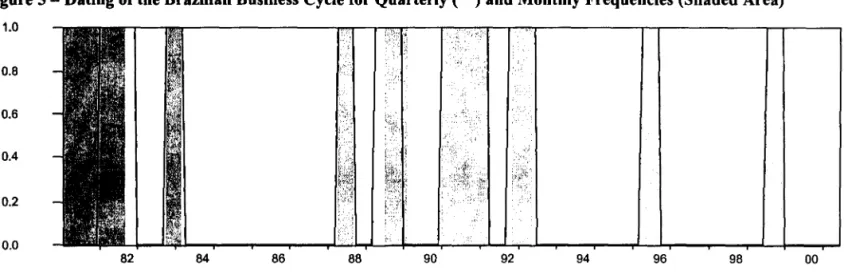
Figure S - Dating of the Brazilian Business Cycle for Quarterly (-) and Monthly Frequencies (Shaded Area)
1.0 iiiI MA" I 1ft I I I i ',1, . ".1 I e I I I I I
0.8
0.6
0.4
0.2
0.0
82 84 86 88 90 92 94 96 98 00
Figure 6 - Smoothed Probabilities of Recessions and Dating of the Brazilian Business Cycle (Shaded Area)
1.0 iIii&Ii lill ífi'0Mill\ t , li 1\ M
0.8
0.6
0.4
0.2
0.0
76 78 80 82 84 86 88 90 92
•
•
•
•
•
•
•
•
•
•
•
•
•
•
•
•
•
•
•
•
•
•
•
•
•
•
•
•
•
•
•
•
•
•
•
•
•
•
•
•
•
•
•
•
•
•
•
~
"
Figure 4 plots the smoothed probabilities of recessions from the monthly series
combined into the dynamic factor, and the smoothed probabilities of recessions for quarterly
GDP, obtained from Chauvet (2000).18 The probabilities are very similar. In particular, alI
recessions are captured by both models, and the timing and duration of the business cycle
phases are very close. Dne difference is the first recession of the quarterly sample, in
1980-82. Since the sample for quarterly GDP starts only in 1980:01, it captures less information
about this reeession period than the dynamie faetor model, whose sample begins in 1975:01.
The smoothed probabilities ean be used as a metric to identify historical business
eye le turning points in Brazil. Dne mIe is to eonsider that the economy is in a reeession if
the smoothed probabilities of recession are above 50%. Alternatively, the frequeney
distribution of the probabilities can also be used to define a turning point - a mIe of thumb to
eall a peak is when the probabilities of reeessions are greater than their mean plus one-half
their standard deviation. Figure 5 shows turning points of the monthly dynamie faetor and
business cycle dating from GDP, obtained from Chauvet (2000). Either of these mIes results
in very similar dating of expansions and reeessions for both models.19
Figure 6 shows the smoothed probabilities of recessions and the dating of the
Brazilian business cycle at the month1y frequeney (shaded area). In the last 25 years Brazil
experienced ten recessions and ten expansions. Recessions are generally shorter than
expansions. In the sample studied, there were five reeessions lasting only six months while
the longest reeession occurred between 1980 and 1982, lasting 20 months. The longest
expansion took place between 1983 and 1987, while the shorter one (6 months) occurred in
between the recession induced by the Collor's Plan in 1990-1991 and the subsequent
recession in the end of 1991 and beginning of 1992.
Monthly Indicator of GDP
The resulting dynamic factor extracted from the model, Ftlb is the monthly indicator
of Brazilian GDP. Table 3 presents some statistics for the indicator and its components. AlI
18 The quarterly smoothed probabilities were converted to monthly frequency using the quadratic-match average method.
19 In order to rule out short-term events. such as strikes, tax law cbanges, etc. from a broad recession in the economy, one of the NBER rules is that a recession corresponds to a general downtum in lhe economy of at least six months. Here we also consider the minimum duration ofbusiness cycle phases to be six months.
•
•
•
•
•
•
•
•
•
•
•
•
•
•
•
•
•
•
•
•
•
•
•
•
•
•
•
•
•
•
•
•
•
•
•
•
•
•
•
•
•
•
•
•
•
•
•
•
•
components are pro-cyclical, hence displaying a positive correlation with the indicator. The
growth rate of the coincident indicator, ãFtIt, is highly correlated with ãHours (0.87),
followed by Mlroduction (0.61). The other components ãCapacity and ãEmployment have
a balanced contribution to the indic ator, with a correlation around 52%. The least correlated
is ã Wages (0.47).
Statistics
Ftlt in levei
-ãFtlt qoarter\y (*) 1âF tlt montbly
-âCapacity 0.522âHours 0.871
âWages 0.474
ãEmployment 0.512
âProduction 0.611
âGDP qoarterly 0.705
GDP 0.973 (**)
102.062 0.104 0.027 -0.003 -0.127 -0.077 -0.099 0.176 0.493 101.81
Standard Deviation
14.088 2.041 1.070 2.243 1.588 2.495 0.676 3.998 2.279 14.221 (*) Here Mtlt was converted to quarterly frequency for comparison with 6GDP. (**) This is the correlation of GDP with the coincident indicator in leveI, Ftl>
In order to compare the results with GDP, two altemative procedures were
undertaken. First, monthly variables were converted to quarterly frequency using simple
average. Second, GDP was converted to monthly frequency using the local quadratic
interpolation method with average matched to the observed data. The growth rate of the
indicator displays a 70% correlation with GDP at the quarterly frequency.
Figure 7 plots the growth rate of the dynamic factor indicator and the growth rate of
GDP at the monthly frequency. The shaded areas represent recession phases. The
estimated indicator is strongly related to movements in GDP. In particular, the volatility of
these two series is very close, as well as the timing of changes and amplitude of the
oscillations. One exception was the abrupt change in the economy during the Collor Plano
The monthly indicator matches the steep drop in the economic activity upon the introduction
of the Plan in the second quarter of 1990, when GDP decreased at a quarterly average rate
of -6.7%. The indicator, however, did not go up as much as GDP did in the third quarter
•
•
•
•
•
•
•
•
•
•
•
•
•
•
•
•
•
•
•
•
•
•
•
•
•
•
•
•
•
•
•
•
•
•
•
•
•
•
•
•
•
•
•
•
•
~
•
s
•
(6.8%). An analysis of the components of the dynamic factor explains this. Neither
employment, wages nor hours displayed this strong upswing after the frrst impact of the
Collor plano In fact, only industrial production rebounded back. Thus, the indicator reflects
more accurately the negative impact of the plan in the Brazilian labor market. The series on
GDP per sector, obtained from IBGE, corroborates this fmding - the responses of GDP
from the service and agricultural sectors to the Collor Plan were much smoother than the
one from industrial GDP.
Figures 8 and 9 show the estimated indicator in leveI at the monthly and quarterly
frequency, respectively. The indicator in evel was obtained directly from the Kalman filter
using the identity E-l = dFt_1
+
Ft_2 in the filter.20 The indicator follows closely cyclicalmovements in GDP. In particular, the timing of business cycle peaks and troughs coincides
for alI recessions in the sample. Conformity with the reference cycle in terms of the turning
points is one of the most important contributions of the indicator, since it can be used as a
monitoring tool to assess the state of the business cycle.
20 For graphical comparison, the factor is adjusted to bave the same trend as GDP.
~,
UOTECA MARIO
HWRlaUi:.
SIMUNstf."~
::mm~cM
GETUliO
VARGl~
•
•
•
•
•
•
•
•
•
•
•
•
•
•
•
•
•
•
•
•
•
•
•
•
•
•
•
•
•
•
•
•
•
•
•
•
•
•
•
•
•
•
•
•
•
~
~
~
'"
Figure 7 - Monthly Indicator of Brazilian GDP (-), Growth Rate of Real
GDP (-), and Recession Phases (Shaded Area)
10
~---~
5
o
-5
-10
Figure 8 - Indicator ofBrazilian GDP
inLevei (-), Real GDP (-), and
Recession Phases (Shaded Area) at Monthly Frequency
130
120
110
100
90
80
70
82
84
86
8890
92
9496
98
21
•
•
•
•
•
•
•
•
•
•
.,
•
•
•
•
•
•
•
•
•
•
•
•
•
•
•
•
•
•
•
•
•
•
•
•
•
•
•
•
•
•
•
•
•
•
•
•
~
L,
Figure 9 - Indicator ofBrazilian GDP (-), Real GDP (-), and Recession Phases
(Shaded Area) at Quarterly Frequency
130
120
110
100
90
80
70
82
84
86
88
90
92
94
96
98
00
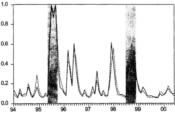
Figure 10 - Out-of-Sample (-) and In-Sample (-) Filtered Probabilities of
Recession, and Recession Phases (Shaded Area)
1.0
...---""õ""'T'"---,---,
0.8
0.6
0.4
0.2
0.0
-i-TTTTTTTTnrTTT"rT194
•
•
•
•
•
•
•
•
•
•
•
•
•
•
•
•
•
•
•
•
•
•
•
•
•
•
•
•
•
•
•
•
•
•
•
•
•
•
•
•
•
•
•
•
•
•
•
•
•
4.3
Out-of-Sample Analysis
The in-sample analysis shows a remarkable historical conformity of the indicator
with cyclical movements of GDP. In this section, the conformity of the indicator as well as
its linear forecasting ability are verified out-of-sample.
In this exercise, the model is estimated fiom 1975:02 to 1993:12. The model is then
recursively re-estimated for each month fiom 1994:01 to 2000:06 and out-of-sample
recursive forecasts of the filtered coincident indicator and probabilities are computed. This
tests the ability of the indicator to predict GDP business cycle phases out-of-sample in real
time, and allows us to reproduce the information content that was available to forecasters at
any point in time.
Probabilities
Figure 10 compares the in-sample probabilities recessions obtained fiom estimating
the model for the entire sample with the out-of-sample filtered probabilities of recession.
Both probabilities are very similar. In particular, the out-of-sample probabilities predict the
two recessions in the period, in 1995 and in 1998. The out-of-sample probabilities,
however, exhibit more pronounced spikes during the short-lived contractions that occurred
in mid-1996 and in the end of 1997. Although these events are not considered recessions
given their mildness and short length (only three montbs), they illustrate the harder task of
discerning in real time false peaks fiom signals of more severe upcoming recessions.
Linear Forecasts
Composite indicators are generally used to predict expansion and recessions phases.
The indicators, however, have also been shown to display good linear predictive power to
forecast output as well.21 This section explores the linear forecasting ability of the monthly
indicator. Two linear models are used to evaluate the performance of the indicator (Mtlt) in
predicting growth rates of GDP (~GDP).22 Model A is a regression of ~GDP on six lags of
itself, and Model B is a vector autoregression of ~GDP and Mtjt at six lags.23 The
21 See Diebold and Rudebusch (1989,1991), Hamilton and Perez-Quiros (1996), etc.
Z2 Since the two series have different frequencies, the indicator was converted as quarterly using simple
average.