www.ann-geophys.net/26/1641/2008/ © European Geosciences Union 2008
Annales
Geophysicae
Iterative inversion of global magnetospheric ion distributions using
energetic neutral atom (ENA) images recorded by the NUADU/TC2
instrument
L. Lu1, S. McKenna-Lawlor2, S. Barabash3, K. Kudela4, J. Balaz2,4, I. Strharsky2,4, Z. X. Liu1, C. Shen1, J. B. Cao1, P. C. Brandt5, C. L. Tang6, and I. Dandouras7
1Centre for Space Science and Applied Research of the Chinese Academy of Sciences, Beijing, China 2Space Technology Ireland, National University of Ireland, Maynooth, Co. Kildare, Ireland
3Swedish Institute of Space Physics, Kiruna, Sweden 4Institute of Experimental Physics, Kosice, Slovakia
5The Johns Hopkins University Applied Physics Laboratory, Laurel MD, USA
6School of Earth and Space Sciences, University of Science and Technology of China, Hefei, China 7Centre d’Etude Spatiale des Rayonnements, Toulouse, France
Received: 16 November 2007 – Revised: 2 April 2008 – Accepted: 18 April 2008 – Published: 11 June 2008
Abstract.A method has been developed for extracting mag-netospheric ion distributions from Energetic Neutral Atom (ENA) measurements made by the NUADU instrument on the TC-2 spacecraft. Based on a constrained linear inversion, this iterative technique is suitable for use in the case of an ENA image measurement, featuring a sharply peaked spa-tial distribution. The method allows for magnetospheric ion distributions to be extracted from a low-count ENA image recorded over a short integration time (5 min). The technique is demonstrated through its application to a set of representa-tive ENA images recorded in energy Channel 2 (hydrogen: 50–81 keV, oxygen: 138–185 keV) of the NUADU instru-ment during a geomagnetic storm. It is demonstrated that this inversion method provides a useful tool for extracting ion distribution information from ENA data that are charac-terized by high temporal and spatial resolution. The recov-ered ENA images obtained from inverted ion fluxes match most effectively the measurements made at maximum ENA intensity.
Keywords. Magnetospheric physics (Energetic particles, trapped; Storms and substorms) – Space plasma physics (Nu-merical simulation studies)
Correspondence to:L. Lu ([email protected])
1 Introduction
Energetic Neutral Atom (ENA) imaging is currently estab-lished as a powerful method for providing a global charac-terization of the Earth’s ring current. NUADU is a dedi-cated ENA instrument flown on the TC-2 spacecraft, which is in an elliptical polar-orbit (700×39 000 km) around the Earth at an inclination of 90◦. TC-2 spins about its axis, which is orientated toward the ecliptic pole, thereby provid-ing NUADU with the capability to image ENAs over a 4π
solid angle. Each image provides global information con-cerning ENAs emitted through the charge exchange process. Conventional charged particle measurements are, in contrast, obtained through in-situ measurements.
Each ENA image contains a great deal of information about the magnetosphere, in particular, about the sources of ENAs generated (via charge exchange) between energetic ions spiraling around the geomagnetic field lines and ambi-ent, cold, neutral particles of the exosphere. The informa-tion contained in such images is, however, difficult to extract directly and quantitative techniques for processing and pre-senting this information are required in order to make such images truly useful.
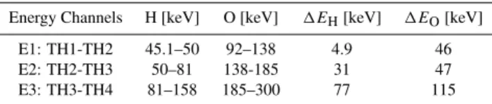
Table 1.Energy channels of NUADU.
Energy Channels H [keV] O [keV] 1EH[keV] 1EO[keV]
E1: TH1-TH2 45.1–50 92–138 4.9 46
E2: TH2-TH3 50–81 138-185 31 47
E3: TH3-TH4 81–158 185–300 77 115
the inversion problem. Validation of this latter method was achieved through comparing ion fluxes retrieved by invert-ing ENA images with those measured in situ by the Cluster constellation (Vallat et al., 2004).
Many papers concerning the analysis of extracted mag-netospheric ion distributions based on HENA/IMAGE mea-surements have already been published (e.g. Brandt et al., 2002a and b; Perez et al., 2004; Zhang et al., 2005). In these retrievals, the ENA images were integrated for at least 10 minutes to achieve adequate counting statistics.
The NUADU instrument has, since the launch of TC-2 in 2004, been monitoring, with high temporal and spatial res-olution, the magnetospheric ENA emissions that accompany geomagnetic storms (a one frame ENA image covering a full 4π solid angle is recorded every four seconds with a spa-tial resolution 11.5◦×2.5◦). Generally, typical ENA images are recorded for about an hour outside the radiation belts near apogee during magnetic storms. These ENA image data (typ-ical integration time 16 s) display inherent fluctuations due to the limited statistics of ENA sampling in the short inte-gration time, thus accruing to each pixel. Nevertheless, in these images we can identify an obvious evolution sequence in the area of maximum ENA emission. After a long-time integration, an ENA image is obtained that displays a sharp ENA maximum distribution within a relatively smooth and low ENA emission background. Previous inversion meth-ods are not suitable to process such image data due to the strong coefficient of constraint associatively employed that may smooth the inverted ion flux distribution unduly and, thereby, inhibit the proper recovery of the ENA image within its area of maximum emission. The iterative technique ap-plied and described in the present paper extracts and accu-mulates characteristic ENA information from step solutions, and the iterative process associatively employed is moni-tored through consideration of the relative errors pertaining between the recovered ENA image and the image obtained through actual measurement. Also, the iterative technique is configured to be tolerant of the inherent noise background and this enables us to investigate the evolution of magneto-spheric ion flux distributions through investigating a set of ENA images recorded, while employing a relatively short in-tegration time, during a magnetic storm.
A brief description of NUADU measurements is presented in Sect. 2. Section 3 provides the basic equations governing these measurements. Simulated images are shown in Sect. 4.
The retrieval method is applied, discussed and evaluated in Sects. 5 and 6 contains a summary and general conclusions.
2 NUADU measurements
The Energetic NeUtral Atom Detector Unit (NUADU) aboard TC-2 features 16 solid-state detectors, each with an equal field of view (11.5◦×2.5◦ FWHM), distributed uni-formly over a 180◦angle in the elevation plane. Spacecraft spin allows the azimuthal plane to be divided into 128 equal sectors, by counting timing pulses provided by the space-craft, so that NUADU completes a full 4π image of the am-bient particle population by the end of each spacecraft spin (4 s). It is possible to integrate data obtained inN spins on-board within the rangeN=2−32 to achieve better statistics. The ENAs measured during individual spins are separated into 3 energy channels (Table 1). (See McKenna-Lawlor et al. (2004) for a more detailed description of the NUADU in-strument.)
NUADU counts individual ENAs without mass discrim-ination and, under most circumstances, the instrument has a low noise background. Under disturbed conditions, op-eration of the instrument in toggle mode (when the output voltage is toggled between 0 and +/−5000 V) , allows the in-strument to measure ENAs when the high voltage is ON and ENAs plus charged particles when the high voltage is OFF. The simulated cutoff energy of the NUADU deflection sys-tem with nominal deflection voltage (10 kV) is 320 keV for singly charged particles. The measured ENA fluxes include hydrogen and other heavy neutrals (mainly oxygen).
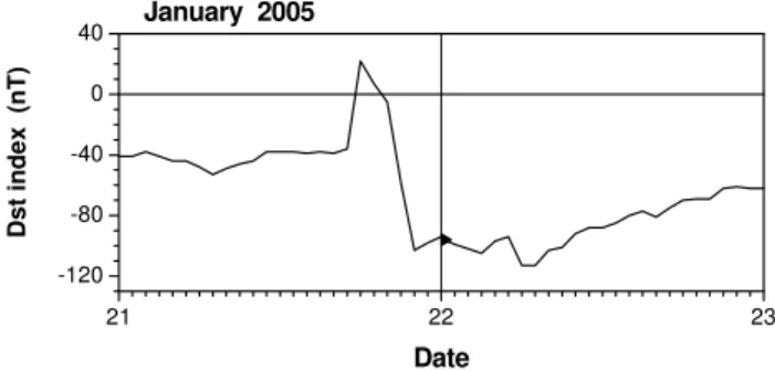
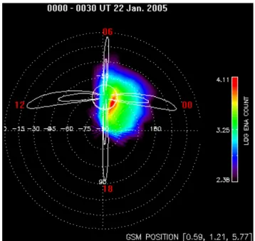
The NUADU image, Fig. 1, used herein to test the in-version technique, was obtained by integrating ENA data recorded during 452 spacecraft spins (30 min) in energy Channel 2 of NUADU during the main-phase of a geo-magnetic storm which attained a maximum Dst=−113 nT
Fig. 1.ENA image (left panel) recorded by NUADU on 22 January 2005 from 00:00 to 00:30 UT in energy Channel 2. The elevation scale is indicated by closed dashed white rings and the azimuth scale by (labeled) dashed lines. The color scale indicates the logarithm of particle counts. Solid white curves represent constant L-values (L=4, 8). Four local times are shown in red. ENA-count distributions are plotted to the right vs. azimuth (top) and elevation (bottom), where red curves relate to the ENA intensity maximum, and black and green curves relate to locations closely surrounding the location of ENA maximum.
admissible value during ion flux inversion). The position of the spacecraft during the measurements is indicated at the bottom of the left panel of Fig. 1 in units ofREand in GSM
coordinates. The ENA count maximum at the nightside was distributed in a narrow area with a rather sharp boundary close to the profile of the Earth (the solid white ring in the left panel of Fig. 1). The shadow of the Earth is represented within the solid white ring by brown-purple and by black col-ors. The bright region, seen mainly around the outside of the profile of the Earth, is interpreted to be due to ENA emissions from the magnetic L-shells external toL=4.
3 Simulation equations
Simulation bins for the ENA source were established by di-viding the magnetic L-shells (from L=2 to L=8) into seg-ments of equal longitude and latitude in the GSM nate system. Each volume element was assigned coordi-nates described by its L-shell longitudeϕand latitudeθ. The space outside the simulation bins was assumed to be an op-tically thin medium with respect to ENA flux, so that ENAs could travel along the line-of-sight (LOS) without undergo-ing charge-exchange.
21 22 23
-120 -80 -40 0 40
Dst index
(nT)
Date January 2005
Fig. 2.The development of theDst index on 21–22 January 2005. Between 00:00–01:00 UT , (marked with a black triangle), theDst index was about−99 nT.
The counts recorded in each pixel of an ENA image,Cδ,ε
(pixel with elevationδand azimuthε), is represented in the simulation system by the equation
Cδ,ε=
Z
dV 1E1T 1A(δ, ε)[jionHσH(E)+jionOσO(E)]n,
(1) wheredV is the volume element of the LOS of each pixel;
+X
-X TO NORTH ECLIPTICAL POLE
TO SOUTH ECLIPTICAL POLE
EQUATORIAL PLANE
S/ C SP IN A XI S 8 15 5 5.6°11.25° 11.25°
SINGLE DETECTOR FOV DEFINITION
POINTING DIRECTIONS OF THE DETECTORS
14.2 DETECTOR 14.2 x 10
INPUT APERTURE
46 x 10
10 46 10 DET4 DET3 DET2 DET1 DET5 DET6 DET7 DET8 DET9 DET10 DET11 DET12 DET13 DET14 DET15 DET16 228 D E FL E C TO R PL A T E + 5 0 0 0V DEF L ECT O
R PLA
T E -5 000 V
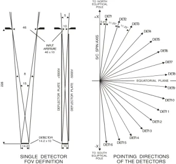
Fig. 3. Geometry of the detectors of the NUADU instrument. (Left), definition of the field of view of a single detector; (Right) pointing directions of all 16 detectors.
detected;1is the solid angle of the volume element point-ing to theδ,εpixel;A(δ, ε) is the response function of a de-tector at that pixel with elevationδand azimuthε,jionHand
jionO are the unknown ion fluxes of hydrogen and oxygen;
σH(E)andσO(E)are the respective charge exchange cross sections between energetic hydrogen and energetic oxygen ions and cold exospheric neutral atoms and n is the exo-spheric neutral atom density near Earth. Integration is along the LOS of the instrument (note that in the analysis of our data we only consider charge exchange between hydrogen atoms, which comprise the dominant exospheric species). 3.1 Detector response function
Figure 3 describes the geometry of the NUADU detectors. In this system, the ENA flux was emitted from an Earth-based volume element (at longitudeϕ, magnetic latitudeλ, andL)
with elevationδ∗and azimuthε∗pointing to the volume el-ement from the sensor. The simplest response coefficient of the pixel with normal directionδ andεat the center of the pixel is given by
Aϕ,λ,L(δ, ε)=ef(δ)
bhcos1δcos1ε Sϕ,λ,L
, (2)
whereef(δ)is the efficiency factor,Sφ,λ,Lis the cross
sec-tion of the volume element perpendicular to the line-of-sight,
1δ= |δ∗−δ|,1ε= |ε∗−ε|, the detector-response-length,
h, is
h=0, 1ε≥2.5◦
h=1.0−22.8 tan1ε,0◦< 1ε <2.5◦, (3)
and the detector-response-width,b, is
b=0, 1δ≥7.5◦
b=3.01−22.8 tan1δ, 4◦< 1δ <7.5◦
b=1.42, 1δ≤4◦.
(4)
The efficiency factor,ef(δ)=Ef(δ), where,Ef(δ)≈0.91 for
each detector (determined from calibration). 3.2 Magnetospheric ion flux
On combining variances of energy, pitch angle and magnetic
Lindex, an empirical model of the ion flux in the ring current region deduced from a Kappa distribution (Christon et al., 1991) may be expressed in the form (Shen, 2002)
jion(L, ϕ, λ, E, α)=ej0(L, ϕ) E E0
1+ E (L/L0)
3 κE0
!
[sinαeq+ 1−sinαeq(L0/L)0.45]2
−κ−1
, (5)
where e=(1+1/κ)κ+1≈2.962 (κ=5.5) (Christon et al., 1991), λ is the magnetic latitude, E0 (7 keV for protons, 16 keV for oxygen ions) (Shen, 2002) is the typical ion-energy of the maximum ion-flux, and L0=7.3 is the outer
boundary of the ion injection region of the ring current (RC). The pitch angle (α) of the particles within the volume ele-ment is expressed in terms ofλ(magnetic latitude) andαeq
(equatorial pitch angle), such that sinα=(1+3 sin
2λ)1/4
cos3λ sinαeq. (6)
Since in the absence of mass analysis the proton flux distri-bution cannot readily be separated from the oxygen ion flux, both are combined in the inversion Eq. (1) to reflect a mixed ion component,j∗(L, ϕ, λ, E, α), as:
j∗(L, ϕ, λ, E, α)σ∗(E)≡jionH(L, ϕ, λ, E, α)σH(EH)+jionO(L, ϕ, λ, E, α)σO(EO)
=ej∗
0(L, ϕ)
jH0σH(EH)EH
EH0
1+ EH L
L0
3
κEH0
!
[sinαeq+ 1−sinαeq
L0L0.45]2
!−κ−1
+jO0σO(EO)EO EO0 1+
EO L
L03 κEO0
!
[sinαeq+ 1−sinαeq L0L0.45]2 !−κ−1
,
(7) wherej0∗(L, ϕ) represents the dimensionless unknown part of the ion-flux introduced to appropriately modify the distri-bution, andjH0andjO0are the initial inputs of ion fluxes for protons and oxygen ions with empirical constants.
3.3 Neutral density of the exosphere
In general, neutral hydrogen is dominant in the exosphere and we have only considered charge exchange with exo-spheric hydrogen atoms. Its density, according to Rairden et al. (1986) and Brandt et al. (2002a), in an adjusted Cham-berlain model is represented by
n(r, ϕ, θ )=3300 exp
17.5e−1.5r− r
H (ϕ, θ )
where
H (ϕ, θ )=1.46(1−0.3 sinθcosϕ) . (9) Here,ris the geocentric distance,ϕ is the local time angle from noon andθ is the polar angle from the z-axis in the GSM coordinate system. The coefficient of 0.3 in Eq. (9) allows one to represent the geotail in the approximated form of an axis-symmetric (around the Sun-Earth line) exosphere. All numeric coefficients in the above expressions have been obtained from the fit to the Chamberlain model by Rairden et al. (1986) and Brandt et al. (2002a). We would like to stress that although the existence of a geotail is confirmed, quantitative knowledge concerning it is presently sparse. 3.4 Numerical quadrature format
The integral in Eq. (1) can be calculated numerically along the line-of-sight so that
Cδ,ε =1T 1E
X
j
1i,j,kAi,j,k(δ, ε)ji,j,k∗
(L, λ, ϕ, E, α)σ∗(E)n0(L, λ)j,k1Vi,j,k, (10)
whereirepresents theϕcoordinate,j theλcoordinate andk
theLcoordinate of the volume element.
The summation operation yields, viaj, a set of linear al-gebraic equations which can be written in (matrix) form
(C)p=(K)q×p J∗0(L, ϕ)
q. (11)
where K is the coefficient matrix with elements of the quadrature weights computed from Eq. (10), and J∗0(L, ϕ)
is a column matrix with elements j0∗(L, ϕ), as defined in Eq. (7), Sect. 3.2. In Eq. (11) the subscripts to the parenthe-ses indicate the dimensions of the matrices, wherep<δ×ε
andq≤i×kdepend on the number of volume elements and on the number of pixels related to the source of ENAs gener-ated through charge-exchange.
4 ENA image simulation from empirical models
We now use the equations developed in the previous sec-tion to simulate NUADU measurements. During a storm, the oxygen ion flux is usually enhanced so that it exceeds the level of proton flux by about 10% (Lennartsson and Sharp, 1982; Mitchell et al., 2003). In-situ measurements made by RAPID/Cluster after the Cluster spacecraft entered the mag-netosphere at 13:00 UT on 22 January (that is on the same day, but after the ENA measurements presented in Fig. 1 were recorded) are shown in Fig. 4. Before 13:00 UT, the Cluster spacecraft operated in the solar wind on the dayside. Figure 4 shows that the mean integral heavy ion flux aver-aged over 4π(E>90 keV), mainly in oxygen ions, was about 5.7×10⁴s−1sr−1cm−2 while the mean integral proton flux averaged over 4π (E>27 keV) was 4×10⁵s−1sr−1cm−2. These species maintained this ratio during the evolution in a
14:00 16:00 18:00 20:00 22:00 24:00
102 103 104 105 106
Io
n Fl
u
x
(
c
m
-2 sr -1 s -1 )
22 January, 2005 Proton (E>27 keV)
Heavy Ion Flux (E>90 keV)
Fig. 4.Integral ion fluxes averaged over 4πby the RAPID/Cluster instrument within the magnetosphere, where the black curve repre-sents proton fluxes (E>27 keV) and the red curve heavy ion fluxes (E>90 keV).
composition that occurred during the remainder of the day. Further, as the Cluster spacecraft (C#3) crossed the equa-torial plane atL=4.2 dusk-night sector at 20:52 UT (while
Dst=−69 nT in the recovery phase of the storm), the
in-tegral heavy ion flux averaged over 4π (E>90 keV) was 4.1×10⁵s−1sr−1cm−2, and the integral proton flux
aver-aged over 4π (E>27 keV) was 2.9×10⁶s−1sr−1cm−2(i.e.
it was about 7 times higher than the former value). Thus, the preliminary parameters’ input to the simulation was set at 4×10⁵ and 5.7×10⁴s−1sr−1cm−2keV−1, respectively, for the proton and oxygen ion fluxes. That is,
jH0(L, ϕ, λ, E, α)=4×10⁵ EH EH0 1+
EH LL03 κEH0
!
[sinαeq+ 1−sinαeq L0L 0.45
]2
−κ−1
h(ϕ) (12) and
jO0(L, ϕ, λ, E, α)=5.7×10⁴EO
EO0
1+ EO L
L03 κEO0
!
[sinαeq+ 1−sinαeq L0L 0.45
]2−κ−1h(ϕ), (13) where h(ϕ)=exp [−0.75(1−cos(ϕ−ϕs))], ϕs is the
az-imuth angle shifted to the location where the intensity of the ring current (RC) particles showed its maximum value; the relevant charge exchange cross sections are
σH=2×10⁻¹⁷cm2andσO=8×10⁻¹⁶cm2(Smith and Bewtra,
1987).
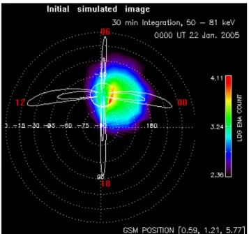
Figure 5 shows the results of a simulation of NUADU measurements made for 22 January 2005. The azimuth angle
ϕs was chosen to be 160◦, so that the ENA maximum was in
Fig. 5.Initial simulated ENA image displayed using the same for-mat utilized in the left panel of Fig. 1.
colored areas in Fig. 5 define the signatures of ENA counts recorded from the near-Earth magnetosphere, as seen in a 4π
solid angle view.
Although it is difficult (Sect. 1) to derive information, even qualitatively, directly from an ENA image, a recovery tech-nique is presented below which is designed to retrieve from the NUADU data within the prevailing constraints, the ion distributions corresponding to the measured ENA images. In the absence (see above) of mass analysis we have to assume the initial ion flux ratio between protons and oxygen ions and extract a mixed distribution based on the empirical model and this assumption.
In the mixed ion component inversion method described below, the maximum ion flux depends on the total percentage of oxygen ions present. Since the charge exchange cross sec-tion of oxygen ions is one order of magnitude higher than that pertaining in the case of protons, oxygen ions are more effec-tive in generating ENA emissions than are protons. Thus, the higher the percentage of oxygen ions present, the lower the maximum mixed ion flux is that will be inverted.
5 Constrained linear inversion by iteration
In a strict sense, Eq. (11) can only be solved uniquely if the matrix K is at once square and non-singular. In practice these two criteria cannot be met simultaneously. Instead of seek-ing a direct solution, we pursue a least-squares method under constraints (see also DeMajistre et al., 2004); i.e. we deter-mineJ0∗through minimizing the quantities
C−KJ∗0T σ−2
C C−KJ
∗ 0
+γJ∗0THJ∗0, (14)
whereσ−2
C is the inverse of the measurement covariance
ma-trix, γ is the constraint strength and His a constraint ma-trix (here,H=H0=I, is adopted as the first order constraint
matrix in an iterative solution). For NUADU data,σ−2 C is a
diagonal matrix whose elements are 1/σi2, whereσiis the
un-certainty corresponding to each pixel. Minimizing Eq. (14) yields
J∗0=KTσ−2
C K+γH
−1
KTσ−2
C C. (15)
When applied to NUADU measurements, the results of a lin-ear least-squares solution were found to oscillate, and even to present negative solutions. To solve this problem we in-creased the constraint strength (this approach will be dis-cussed further in Section 5.1), and also limited the oscilla-tory solution region through introducing a mapping-function written as
x∗(x)= 1+ξxmaxx−xmean−xmin, (0≤ξ ≤1) , (16) where x indicates a set of linear least-square solutions of Eq. (15) andxmax is the maximum,xminthe minimum and xmeanthe mean of this set of step oscillatory solutions,ξ is a step-length coefficient, andx∗is a temporary solution which has a limited solution region 0<x∗<2 around 1. The ion flux distributionJ∗0 could then be approached through an itera-tive process (which will be described in Sect. 5.2) using the dimensionless temporary solution x∗ as JH0(n+1)=J(n)H0x∗ and J(nO0+1)=J(n)O0x∗, where superscriptnindicates the iterative se-quence,JH0andJO0 indicate the background inputs of ion
fluxes for protons and oxygen ions, which are equivalent to the initial inputs ofjH0andjO0in Eq. (7).
Instead of comparing the inversion results with the mea-surement covariance (see DeMajistre et al., 2004), we opted instead to compare the inversion results directly with the measurements. The effect of each converging step (con-straint strength variances) could then be justified and mon-itored by adopting a relative error
¯
ER=
s
C−KJ∗0T C−KJ∗0
CTC . (17)
To better represent properties of the maximum ENA distri-bution, we chose to include in the statistics only those pixels having measurements above the average count of 240. The relative error minimum then attained among the iterations (constraint strength variances) represents the optimal ion dis-tribution solution. The value of the relative error depends on the number of pixels taken into account in the statistics. 5.1 Constrained linear inversion
0.044 0.048 0.052 0.056 0.060 0.430
0.435 0.440 0.445 0.450
Relative e
rr
o
r
Gamma Minimum=0.432
Fig. 6.Relative error variance for different constraint strengths.
was obtained (Fig. 6). It is noted that relatively low constraint strengths resulted in a high ion flux solution, whereas rela-tively high constraint strengths resulted in low ion-flux solu-tions. The higher the empirical ion fluxes input, the higher the constraint strengths were, resulting in an optimal solu-tion.
The extracted equatorial ion flux with pitch angle 90◦ at the optimal constraint strength was found to be dis-tributed rather smoothly with a maximum intensity of 1.56×10⁶s−1sr−1cm−2keV−1 (Fig. 7). The most intense patch in the ion distribution was located in the post-dusk sec-tor (L=4) at about 19–20 h local time and it extended toward both dawn and noon with a gap at dusk (which corresponded with measurements of the high polar angle detectors). This result showed a match with the measurements (see the gap at 18:00 MLT in the left panel of Fig. 1), see also the cor-responding recovered ENA image (Fig. 8). The maximum extended outward widely and smoothly in the dusk-night sector, which is also consistent with the extent of the ENA maximum distributions shown in the left panel of Fig. 1 and in Fig. 8. On comparing the recovered image with the left panel of Fig. 1, the maximum ENA count area in the recov-ered image (Fig. 8) was found to be shifted duskward and to be spread more widely, increasing as a result the relative error. It is stressed that the extracted flux was found by vary-ing the constraint strengthγ in Eq. (15) under circumstances where the maximum ENA measured counts were located on the dusk side and the linear constrained method smoothed the inverted ion fluxes around the ENA intensity maximum area. 5.2 Iterative inversion
In order to better represent the properties of the intensity patch in the ENA measurements (left panel, Fig. 1), we next performed an iteration to retrieve the ion distribution through employing a constant constraint strength (γ=0.04) that was smaller than that associated with the optimal solution of the previous section. As already indicated above, the ion
distri-Fig. 7. The optimal equatorial ion distribution contour with pitch angle 90◦, where the closed dashed curves represent the L-scale (2– 8) in Earth radii. Local times and a color scales are provided outside the perimeter of the outermost L-boundary.
Fig. 8. The optimal recovered ENA image displayed in the same format used in the left panel of Fig. 1.
bution sought (J∗
0) could be approached using the temporary
solution x∗, as J(n+1) H0 =J
(n)
H0x∗ andJ (n+1) O0 =J
(n)
O0x∗, where n
indicates the iterative sequence. JH0andJO0 represent the
02 04 06 08 10 0.2
0.3 0.4 0.5 0.6 0.7
Relative e
rr
o
r
Iterative sequence Minimum=0.244 Gamma=0.04
Fig. 9.Relative error variance during an iteration for whichγ=0.04.
Fig. 10.The final equatorial ion distribution contour for pitch angle 90◦, displayed in the same format used in Fig. 7.
The mapping function (Eq. 16) which was associatively introduced, enabled us, through employing a linear, region-limited, artificial solution, to utilize the enhancing ion flux modifications to guide the step-by-step solutions, so that, gradually, they approached the actual measurements of ENA intensity.
The success of the iterative process in improving, after each step, the input of the ion flux background was deter-mined using the relative error Eq. (17) and the same statis-tical pixels considered in Sect. 5.1, until a minimum value (0.24, Fig. 9) was obtained. We can follow in this figure how the solution was adjusted step by step. After the rel-ative error minimum, the error profile was found to rise in approximately the same way in which it fell off (even some-what faster, since the pixels with large ENA counts were still enhanced through the mapping function (Eq. 16)).
The maximum intensity of the extracted equatorial ion flux with pitch angle 90◦at the minimum relative error (0.24) was
Fig. 11.The final recovered ENA image displayed in the same for-mat used in the left panel of Fig. 1.
1.43×10⁶s−1sr−1cm−2keV−1(Fig. 10), which is of about the same order of magnitude as that shown in Fig. 7. The in-tense patches of the ion-flux distribution were shown to have a complex construction featuring relatively sharp boundaries that were consistent with both the measured ENA flux max-imum distribution (left panel, Fig. 1) and the recovered im-age (Fig. 11). The intense ion-flux configuration extended outward on the dusk side but was constricted inward on the night side, which may represent an RC ion distribution re-gion that was compressed earthward during the main phase of the storm (Fig. 2).
0 60 120 180 240 300 360 10
100 1000 10000
E
N
A Co
unt
s
Azimuth (degree)
Measurement Iteration Constraint 240 (mean count)
0 30 60 90 120 150 180
10 100 1000 10000
ENA Co
un
ts
Elevation (degree)
Measurement Iteration Constraint 240 (mean count)
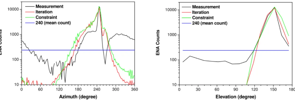
Fig. 12.Comparison of ENA-count distributions versus azimuth (left) and elevation (right) where: the black curves represent the measure-ments shown in Fig. 1 at the ENA intensity maximum; blue lines represent the mean ENA count in Fig. 1; red and green curves represent recovered images from inverted ion fluxes derived, respectively, by iteration (Fig. 11) and by linear constraint (Fig. 8). For further details see the text.
green curve (obtained using the linear constraint scheme) dis-plays a close approach to the black curve (obtained through measurement).
From the viewpoint of relative error statistics with re-spect to the high intensity area, the precision of the itera-tive scheme (with relaitera-tive error 0.244) is higher by a factor of about two than that derived when using linear constraint inversion (relative error 0.432). It is thus inferred that the it-erative technique is the more suitable choice for ion flux ex-traction from an ENA image characterized by a sharp ENA peak.
5.3 Iterative inversions for a short integration time
Since the mapping function Eq. (16) enables us to better cope with oscillatory solutions, the iterative technique can be applied when studying relatively short-integrations of ENA flux measurements made by NUADU during geomagnetic storms. To demonstrate this capability, the method described above is next applied in the case of short integration times. First, we divide the measurements already discussed into six segments and adopt five-minute integration times for each segment (see Fig. 13, which shows the temporal evolution of the ENA measurements concerned). For the same statis-tical pixels as those already considered above, we derived a set of ion-flux distributions with an average relative error 0.2 during the evolution sequence (Fig. 14) and recovered ENA images (Fig. 15) from each extracted ion-flux distribution.
The short integration measurements in Fig. 13 look rather patchy as compared with those shown in the left panel of Fig. 1, but it is still possible to identify structures within the ENA flux maximum (red color) and in the high latitude ENA distributions (bright-blue color). Figure 13 shows that during the evolution process, the five-minute ENA distribu-tions were, especially in the maximum ENA area, initially
enhanced in the first three segments and they then decreased and shifted duskward in the following three segments.
Generally, each ion flux color map in Fig. 14 shared about the same distribution configuration (similar to that seen in Fig. 10), but viewed in detail, the intense ion-flux patches exhibited magnitude changes and shifting locations. The ion-flux distribution in the RC region seems to have displayed a configuration that was initially compressed and then recov-ered during the main phase of the storm (Fig. 2). Figure 15 shows that each recovered ENA image matched well those measurements made (Fig. 13) in the ENA maximum area.
6 Summary and conclusions
Fig. 13. Five minute ENA integration measurements displayed in the same format employed in the left panel of Fig. 1. The epochs are provided at the top of each panel.
Fig. 15. Recovered ENA images from retrieved ion-fluxes using five-minute integration measurements displayed in the same format em-ployed in the left panel of Fig. 1. The epochs are provided at the top of each panel.
By applying the technique to a representative ENA image recorded during a storm, a recovered ENA image was ob-tained that showed a close approach to measured reality in the brightest ENA area.
In brief, a technique was developed to extract magneto-spheric ion distributions contained in ENA data, together with a means to quantify their quality. This method, which was custom developed for NUADU data recorded over a 4π
solid angle, was demonstrated to be applicable in cases of both high and low sensor count rates. It thus constitutes a useful tool for the inversion of global magnetospheric infor-mation from ENA images obtained at high temporal and spa-tial resolution. This method can also support investigations of the evolution of ion-flux distributions extracted from ENA measurements made with short integration times during the development of geomagnetic storms.
The iterative inversion technique described potentially supports the retrieval of magnetospheric ion distributions from multiple ENA images. If, for instance, two ENA im-ages of the ring current were recorded simultaneously from different positions, the ion-flux distribution in the ring cur-rent region could be alternately adjusted between the two measurements so that, ultimately, a unique ion-flux distribu-tion soludistribu-tion matching the two simultaneous measurements could be achieved. The NAIK instruments in the straw man payload of the twin spacecraft of China’s planned Kuafu-B mission can potentially be utilized to accomplish this goal.
Acknowledgements. This study was supported by the Chinese
Na-tional Natural Science Foundation Committee grant 40674083 and 40390153, Chinese National Key Laboratory research outlay grant 40523006. S. McKenna-Lawlor acknowledges with appreciation the support of Enterprise Ireland. K. Kudela thanks the Slo-vak Research and Development Agency for support under contract No. APVV-51-053805 and VEGA grant agency project 2/7063/27. Topical Editor I. A. Daglis thanks two anonymous referees for their help in evaluating this paper.
References
Brandt, P. C., Demajistre, R., Roelof, E. C., Ohtani, S., and Mitchell, D. G.: IMAGE/high-energy energetic neutral atom: Global energeticneutral atom imaging of the plasma sheet and ring current during substorms, J. Gephys. Res., 107(A12), 1454, doi:10.1029/2002JA009307, 2002a.
Brandt, P. C., Roelof, E. C., Ohtani, S., Mitchell, D. G., and An-derson, B.: IMAGE/HENA: Pressure and current distributions during the 1 October 2002 storm, Adv. Space Res., 33, 719–722, 2002b.
Christon, S. P., Williams, D. J., and Mitchell, D. G.: Spectral char-acteristics of plasma sheet ion and electron populations during disturbed geomagnetic condition, J. Geophys. Res., 96, 1–22, 1991.
IMAGE/HENA instrument, J. Geophys. Res., 109, A04214, doi:10.1029/2003JA010322, 2004.
Lennartsson, W. and Sharp, R. D.: A comparison of 0.1-17 keV/e ion composition in the near equatorial magnetosphere between quite and disturbed conditions, J. Geophys. Res., 87, 6109–6120, 1982.
McKenna-Lawlor, S., Balaz, J., Barabash, S., Johnsson, K. Lu, L., Shen, C., Shi, J. K., Zong, Q. G., Kudela, K., Fu, S. Y., Roelof, E. C., Brandt, P. C., and Dandouras, I.: The energetic NeUtral Atom Detector Unit (NUADU) for China’s Double Star Mission and its calibration, Nuclear Inst. & Methods, A(503), 311–322, 2004.
Mitchell, D. G., Brandt, P. C., Roelof, E. C., Hamilton, D. C., Ret-terer, K. C., and Mende, S.: Global imaging of O+from IM-AGE.HENA, Space Sci. Rev., 109, 63–75, 2003.
Perez, J. D., Fok, M.-C., and Moore, T. E.: Deconvolution of en-ergetic neutral atom images of the earth’s magnetosphere, Space Sci. Rev., 91, 421–436, 2000.
Perez, J. D., Kozlowski, G., Brandt, P. C., Mitchell, D. G., Jahn, J. M., Pollock, C. J., and Zhang, X.: Initial ion equatorial pitch angle distributions from energetic netural atom images obtained by IMAGE, Geophys. Res. Lett., 28, 1155–1158, 2001. Perez, J. D., Zhang, X. X., Brandt, P. C., Mitchell, D. G., Jahn,
J.-M., and Pollock, C. J.: Dynamics of ring current ions as obtained from IMAGE HENA and MENA ENA images, J. Geophys. Res., 109, A05208, doi:10.1029/2003JA010164, 2004.
Rairden, R. L., Frank, L. A., and Craven, J. D.: Geocoronal imaging with dynamics explorer, J. Geophys. Res., 91, 13 613–13 630, 1986.
Roelof, E. C. and Skinner, A. J.: Extraction of ion distributions from magnetospheric ENA and EUV images, Space Sci. Rev., 91, 437–459, 2000.
Shen, C. and Liu, Z. X.: Properties of the Neutral Energetic Atoms Emitted from Earth’s Ring Current Region, Phys. Plasmas, 9, 3984–3994, 2002.
Smith, P. H. and Bewtra, N. K.: Charge exchange lifetimes for ring current ions, Space Sci. Rev., 22, 301–318, 1987.
Vallat, C., Dandouras, I., Brandt, P. C., DeMaijistre, R., Mitchell, D. G., Roelof, E. C., Reme, H., Sauvaud, J., Kistler, L., Mouikis, C., Dunlop, M., and Balogh, A.: First comparisons of local ion measurements in the inner magnetosphere with energetic neutral atom mgnetospheric image inversions: Cluster-CIS and IMAGE-HENA observations, J. Geophys. Res., 109, A04213, doi:10.1029/2003JA010224, 2004.