ACPD
14, 4119–4148, 2014Spatially resolving methane emissions
in California
K. J. Wecht et al.
Title Page
Abstract Introduction
Conclusions References
Tables Figures
◭ ◮
◭ ◮
Back Close
Full Screen / Esc
Printer-friendly Version
Interactive Discussion
Discussion
P
a
per
|
D
iscussion
P
a
per
|
Discussion
P
a
per
|
Discuss
ion
P
a
per
Atmos. Chem. Phys. Discuss., 14, 4119–4148, 2014 www.atmos-chem-phys-discuss.net/14/4119/2014/ doi:10.5194/acpd-14-4119-2014
© Author(s) 2014. CC Attribution 3.0 License.
Atmospheric Chemistry and Physics
Open Access
Discussions
This discussion paper is/has been under review for the journal Atmospheric Chemistry and Physics (ACP). Please refer to the corresponding final paper in ACP if available.
Spatially resolving methane emissions in
California: constraints from the CalNex
aircraft campaign and from present
(GOSAT, TES) and future (TROPOMI,
geostationary) satellite observations
K. J. Wecht1, D. J. Jacob1, M. P. Sulprizio1, G. W. Santoni1, S. C. Wofsy1, R. Parker2, H. Bösch2, and J. Worden3
1
Department of Earth and Planetary Sciences, Harvard University, Cambridge, MA, USA
2
Earth Observation Science, Space Research Centre, University of Leicester, Leicester, UK
3
Jet Propulsion Laboratory/California Institute of Technology, Pasadena, CA, USA
Received: 9 January 2014 – Accepted: 23 January 2014 – Published: 14 February 2014
Correspondence to: K. J. Wecht ([email protected])
ACPD
14, 4119–4148, 2014Spatially resolving methane emissions
in California
K. J. Wecht et al.
Title Page
Abstract Introduction
Conclusions References
Tables Figures
◭ ◮
◭ ◮
Back Close
Full Screen / Esc
Printer-friendly Version
Interactive Discussion
Discussion
P
a
per
|
D
iscussion
P
a
per
|
Discussion
P
a
per
|
Discuss
ion
P
a
per
|
Abstract
We apply a continental-scale inverse modeling system for North America based on the GEOS-Chem model to optimize California methane emissions at 1/2◦×2/3◦horizontal
resolution using atmospheric observations from the CalNex aircraft campaign (May– June 2010) and from satellites. Inversion of the CalNex data yields a best estimate for 5
total California methane emissions of 2.86±0.21 Tg yr−1, compared with 1.92 Tg yr−1
in the EDGAR v4.2 emission inventory used as a priori and 1.51 Tg yr−1 in the Cali-fornia Air Resources Board (CARB) inventory used for state regulations of greenhouse gas emissions. These results are consistent with a previous Lagrangian inversion of the CalNex data. Our inversion provides 12 independent pieces of information to constrain 10
the geographical distribution of emissions within California. Attribution to individual source types indicates dominant contributions to emissions from landfills/wastewater (1.1 Tg yr−1), livestock (0.87 Tg yr−1), and gas/oil (0.64 Tg yr−1). EDGAR v4.2 under-estimates emissions from livestock while CARB underunder-estimates emissions from land-fills/wastewater and gas/oil. Current satellite observations from GOSAT can constrain 15
methane emissions in the Los Angeles Basin but are too sparse to constrain emissions quantitatively elsewhere in California (they can still be qualitatively useful to diagnose inventory biases). Los Angeles Basin emissions derived from CalNex and GOSAT in-versions are 0.42±0.08 and 0.31±0.08, respectively. An observation system
simu-lation experiment (OSSE) shows that the future TROPOMI satellite instrument (2015 20
launch) will be able to constrain California methane emissions at a detail comparable to the CalNex aircraft campaign. Geostationary satellite observations offer even greater potential for constraining methane emissions in the future.
1 Introduction
Quantifying greenhouse gas emissions at the national and state level is essential for 25
ACPD
14, 4119–4148, 2014Spatially resolving methane emissions
in California
K. J. Wecht et al.
Title Page
Abstract Introduction
Conclusions References
Tables Figures
◭ ◮
◭ ◮
Back Close
Full Screen / Esc
Printer-friendly Version
Interactive Discussion
Discussion
P
a
per
|
D
iscussion
P
a
per
|
Discussion
P
a
per
|
Discuss
ion
P
a
per
greenhouse gas emissions be brought down to 1990 levels by 2020. The California Air Resources Board (CARB) has identified the importance of reducing methane for com-plying with AB32 (CARB, 2013). It provides a statewide methane emission inventory for enforcement of AB32 (CARB, 2011). However, atmospheric observations from surface sites and aircraft suggest that this inventory may be too low by a factor of 2 or more 5
(Wunch et al., 2009; Jeong et al., 2012; Peischl et al., 2012; Wennberg et al., 2012; Santoni et al. 2014). This is problematic in terms of designing a credible emissions control strategy.
Atmospheric observations play a critical role in measurement, reporting and verifi-cation (MRV) of greenhouse gas emission inventories (NRC, 2010). Surface measure-10
ments are limited in space, and aircraft campaigns are limited in time. Satellite obser-vations have the potential for continuous monitoring of emissions if their sensitivity and coverage is sufficient. In Wecht et al. (2013), we present a new capability developed under the NASA Carbon Monitoring System (CMS) to constrain methane emissions at high spatial resolution over North America by inversion of satellite observations in 15
an Eulerian framework (GEOS-Chem chemical transport model). Here we apply this capability to estimate the fine-scale distribution of emissions in California by using ob-servations from the CalNex aircraft campaign (May–June 2010) as well as from current and future satellite instruments.
Santoni et al. (2014) previously used the CalNex aircraft observations in a La-20
grangian inversion of methane emissions for California, optimizing a total of 8 source types/regions within the state. They derived an optimized statewide emission of 2.4 Tg yr−1, as compared to 1.5 Tg yr−1 in the CARB inventory, and attributed most of the underestimate to livestock emissions. Here we use the same CalNex observations as Santoni et al. (2014) but optimize emissions on the 1/2◦
×2/3◦(∼50 km×50 km) grid
25
of GEOS-Chem, without prior assumption on source types, thus providing a different perspective and a check on the use of different inversion methodologies.
obser-ACPD
14, 4119–4148, 2014Spatially resolving methane emissions
in California
K. J. Wecht et al.
Title Page
Abstract Introduction
Conclusions References
Tables Figures
◭ ◮
◭ ◮
Back Close
Full Screen / Esc
Printer-friendly Version
Interactive Discussion
Discussion
P
a
per
|
D
iscussion
P
a
per
|
Discussion
P
a
per
|
Discuss
ion
P
a
per
|
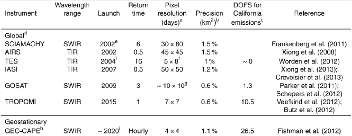
vations. Satellites measure methane from solar backscatter spectra in the short-wave infrared (SWIR) and terrestrial radiation spectra in the thermal infrared (TIR). A num-ber of satellite instruments have the capability to observe methane (Table 1). SWIR retrievals are available from SCIAMACHY (2003–2012) and GOSAT (2009–present). TIR retrievals are available from AIRS (2002–present), TES (2004–2011), and IASI 5
(2007–present). SWIR retrievals provide total atmospheric methane columns. TIR re-trievals provide vertical profiles but have limited sensitivity to the lower troposphere due to lack of thermal contrast, and this limits their value for detecting regional sources (Wecht et al., 2012).
Our initial CMS application described in Wecht et al. (2013) focused on optimiz-10
ing methane emissions on the continental scale of North America using SCIAMACHY observations for summer 2004. SCIAMACHY provided high-quality observations with high density until 2005, after which the sensitivity of the instrument degraded (Franken-berg et al., 2011). Current satellite observations are available from GOSAT and TES. As we will see, these observations are too sparse to usefully constrain the distribution 15
of emissions within California. Drastic improvement in our ability to observe methane from space is expected in 2015 with the launch of the SWIR TROPOMI instrument (Veefkind et al., 2012; Butz et al., 2012). TROPOMI will provide daily global coverage with 7 km×7 km nadir resolution. There are also several current proposals for
geosta-tionary SWIR observation of methane over North America, drawing on plans for the 20
ACPD
14, 4119–4148, 2014Spatially resolving methane emissions
in California
K. J. Wecht et al.
Title Page
Abstract Introduction
Conclusions References
Tables Figures
◭ ◮
◭ ◮
Back Close
Full Screen / Esc
Printer-friendly Version
Interactive Discussion
Discussion
P
a
per
|
D
iscussion
P
a
per
|
Discussion
P
a
per
|
Discuss
ion
P
a
per
2 GEOS-Chem inverse modeling system for methane emissions
2.1 Forward model and optimization procedure
We use the GEOS-Chem chemical transport model (CTM) with 1/2◦
×2/3◦horizontal
resolution as the forward model in the inversion to optimize methane emissions on the basis of observed atmospheric concentrations. The inversion seeks an optimal solu-5
tion for the spatial distribution of methane emissions consistent with both atmospheric observations and a priori knowledge. The a priori is from existing emission invento-ries. The forward model F relates emissions to methane concentrations. Optimization is done by minimizing the Bayesian least-squares cost function,J:
J(x)=(F(x)−y)TS−O1(F(x)−y)+(x−xA)TS−A1(x−xA) (1) 10
Hereyis the ensemble of observations arranged in a vector,SOis the error covariance matrix of the observation system,SAis the error covariance matrix of the a priori
emis-sions,xis a vector of emission scale factors on the 1/2◦×2/3◦GEOS-Chem grid, and xAis the corresponding a priori.xhas as elementsxi =Ei/EA,i, whereEi andEA,i are respectively the true and a priori methane emissions for grid squarei.
15
Analytical solution of Eq. (1) yields the following expression for the optimal estimate ˆ
x, its associated error covariance matrix ˆS, and the averaging kernel matrix A that describes the sensitivity of the retrieved emissions to true emissions (Rodgers, 2000):
ˆ
x=xA+SAKT(KSAKT+SO)−1(y−KxA) (2) ˆ
S−1
=KTS−1 O K+S
−1
A (3)
20
A=In−SSˆ −A1 (4)
Here Kis the Jacobian matrix for the sensitivity of concentrations to emissions cal-culated with GEOS-Chem,In is the identity matrix, andnis the dimension ofx.
We use GEOS-Chem version 9-01-02 (http://www.geos-chem.org/), driven by 25
ACPD
14, 4119–4148, 2014Spatially resolving methane emissions
in California
K. J. Wecht et al.
Title Page
Abstract Introduction
Conclusions References
Tables Figures
◭ ◮
◭ ◮
Back Close
Full Screen / Esc
Printer-friendly Version
Interactive Discussion
Discussion
P
a
per
|
D
iscussion
P
a
per
|
Discussion
P
a
per
|
Discuss
ion
P
a
per
|
(GMAO). The GEOS-5 data have 1/2◦
×2/3◦horizontal resolution, 72 vertical levels
(in-cluding 14 in the lowest 2 km), and 6 h temporal resolution (3 h for surface variables and mixing depths). The simulations are for a nested version of GEOS-Chem with native 1/2◦
×2/3◦ resolution for western North America and the adjacent Pacific (26–70◦N,
110–140◦W) and 3 h dynamic boundary conditions from a global simulation with 4◦×5◦
5
resolution. The transport time step is 10 min. In our previous inverse analysis of SCIA-MACHY observations for North America (Wecht et al., 2013), we used a larger nested domain (10–70◦N, 40–140◦W). Simulations using the two domains show negligible differences over California. The trimmed domain used here makes it computationally feasible to construct the Jacobian matrixKand from there to obtain the analytical so-10
lution Eqs. (2) and (3) with full characterization of error statistics, unlike the numerical solution relying on the GEOS-Chem adjoint as implemented by Wecht et al. (2013). Boundary conditions are treated here by correcting the free tropospheric background to match the CalNex aircraft observations as described in Sect. 3.
The main sink for atmospheric methane is oxidation by OH in the troposphere, and 15
this is computed using a 3-D archive of monthly average OH concentrations from a GEOS-Chem simulation of tropospheric chemistry (Park et al., 2004). Additional mi-nor sinks in GEOS-Chem include soil absorption (Fung et al., 1991) and stratospheric oxidation computed with archived loss frequencies from the NASA Global Modeling Ini-tiative (GMI) Combo CTM (Considine et al., 2008; Allen et al., 2010). Tropospheric loss 20
of methane is inconsequent here since ventilation from the western US window do-main is fast in comparison. Stratospheric loss provides a realistic stratospheric profile of methane and Wecht et al. (2012) pointed out that this is important for the inversion of satellite observations.
2.2 A priori emissions for the inversion
25
A priori anthropogenic emissions in GEOS-Chem are from the EDGAR v4.2 global inventory at 0.1◦×0.1◦resolution for 2008, the most recent year available (EC-JRC/PBL
ACPD
14, 4119–4148, 2014Spatially resolving methane emissions
in California
K. J. Wecht et al.
Title Page
Abstract Introduction
Conclusions References
Tables Figures
◭ ◮
◭ ◮
Back Close
Full Screen / Esc
Printer-friendly Version
Interactive Discussion
Discussion
P
a
per
|
D
iscussion
P
a
per
|
Discussion
P
a
per
|
Discuss
ion
P
a
per
is available from the California Greenhouse Gas Emissions Measurement (CalGEM) Project, described by Zhao et al. (2009) and Jeong et al. (2012). The EDGAR v4.2 inventory on the scale of the US agrees well with the US Environmental Protection Agency (EPA, 2013) national inventory (Wecht et al., 2013). EDGAR emissions are aseasonal but we apply seasonality to California rice emissions following McMillan 5
et al. (2007) with emissions in the growing season (June–September) six times higher than in the rest of the year. Natural emissions include open fires from GFED-3 with daily resolution (van der Werf et al., 2010; Mu et al., 2010) and wetlands with dependence on local temperature and soil moisture (Kaplan et al., 2002; Pickett-Heaps et al., 2011). They account for only 3 % of total a priori methane emissions in California.
10
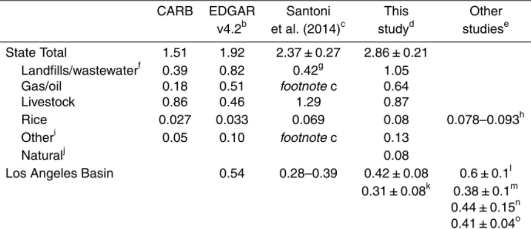
Table 2 shows the statewide emissions in the EDGAR and CARB inventories, with the contributions from different sources. EDGAR emissions are 1.92 Tg yr−1, 27 % higher than CARB emissions of 1.51 Tg yr−1. There are larger discrepancies in contributions from different source types. EDGAR landfills/wastewater and gas/oil emissions are higher than CARB by more than a factor of 2. EDGAR livestock emissions, on the other 15
hand, are lower than CARB by a factor of 2. The CalNex observations can arbitrate on these discrepancies as will be discussed in Sect. 3.3.
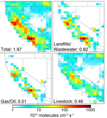
Figure 1 shows the distribution of EDGARv4.2 emissions across California. fill/wastewater and gas/oil emissions closely follow population distribution. Land-fill/wastewater includes landfills (79 %) and wastewater treatment (21 %) with similar 20
spatial patterns in EDGAR. The gas/oil source is dominated by natural gas emissions (94 %) and the correlation with population in EDGAR suggests that it is mostly from distribution rather than extraction, which is concentrated in the southwestern end of the Central Valley. Livestock emissions are mostly in the Central Valley and include both enteric fermentation and manure management.
ACPD
14, 4119–4148, 2014Spatially resolving methane emissions
in California
K. J. Wecht et al.
Title Page
Abstract Introduction
Conclusions References
Tables Figures
◭ ◮
◭ ◮
Back Close
Full Screen / Esc
Printer-friendly Version
Interactive Discussion
Discussion
P
a
per
|
D
iscussion
P
a
per
|
Discussion
P
a
per
|
Discuss
ion
P
a
per
|
3 Inversion of CalNex observations
3.1 Observations and error characterization
Santoni et al. (2014) measured methane concentrations aboard the CalNex aircraft with a Quantum Cascade Laser Spectrometer (QCLS) (Santoni et al., 2013), and de-rived methane emissions from these observations with an inversion using the Stochas-5
tic Time-Inverted Lagrangian Transport (STILT) model. Methane was also measured aboard the CalNex aircraft with a Cavity Ring-Down Spectrometer (CRDS) (Peischl et al., 2012), and Santoni et al. (2014) used these observations to fill gaps in the QCLS record after correcting for bias between the two instruments. They used observations between 2–4 km for each flight to constrain the free tropospheric background, and the 10
observations below 2 km to constrain California emissions. We follow the same ap-proach here, correcting the GEOS-Chem concentrations for the observed free tropo-spheric background on individual days. This effectively accounts for boundary condi-tions. Data selection criteria are described by Santoni et al. (2014).
Figure 2 (left) shows the mean observed methane concentrations below 2 km from 15
the 11 daytime CalNex flights used by Santoni et al. (2014) in their inversion. Values are highest over the Central Valley and the Los Angeles Basin. We use the same observations for our inversion after averaging horizontally, vertically, and temporally over the GEOS-Chem grid. The resulting observation vector y has 1993 elements. We use it to optimize emissions (state vectorx) from the 157 1/2◦
×2/3◦ model grid
20
squares that comprise California. The middle panel of Fig. 2 shows the GEOS-Chem simulation with a priori EDGAR emissions and after correcting for the free tropospheric background. There is a general underestimate and discrepancies in patterns that point to errors in the EDGAR emissions.
We use the residual error method of Heald et al. (2004) to estimate the observational 25
error variances (diagonal elements ofSO). This involves partitioning of the observation
ACPD
14, 4119–4148, 2014Spatially resolving methane emissions
in California
K. J. Wecht et al.
Title Page
Abstract Introduction
Conclusions References
Tables Figures
◭ ◮
◭ ◮
Back Close
Full Screen / Esc
Printer-friendly Version
Interactive Discussion
Discussion
P
a
per
|
D
iscussion
P
a
per
|
Discussion
P
a
per
|
Discuss
ion
P
a
per
Valley, Los Angeles Basin, San Francisco Bay Area, rest of California, and Pacific Ocean. For each subset we assume that the mean difference between observations and the model with a priori sources is caused by error on the a priori sources. The residual standard deviation (RSD) is then assumed to represent the standard devia-tion of the observadevia-tional error. RSD is largest (50–70 ppb) in the lowest 1 km over the 5
Central Valley and the Los Angeles Basin, reflecting small-scale transport and spatial variability in emissions not resolved by the model. RSD below 1 km in other regions is typically 20–40 ppb. RSD in all regions decreases with altitude to 15–20 ppb at 2 km. For each element of y in the subset we populate the diagonal ofSO with the obser-vational error variance, RSD2. Variograms show no significant temporal or horizontal 10
error correlations between observations on the GEOS-Chem grid. We therefore take
SO to be diagonal.
The a priori error covariance matrix,SA, is constructed by assuming a uniform 75 % uncertainty on a priori emissions from every grid square. This magnitude of uncertainty is consistent with the discrepancies between CARB and EDGAR and with the results 15
of Santoni et al. (2014). We assume no error correlations so thatSA is diagonal. Sen-sitivity of the inversion results to specification ofSAis examined in Sect. 3.3.
Care is required to account for model errors in planetary boundary layer (PBL) height. High Spectral Resolution Lidar (HSRL) aircraft observations during CalNex indicated mean midday PBL heights of 1.0 km in the Central Valley and the Los Angeles Basin 20
(Fast et al., 2012). The GEOS-5 meteorological data used in GEOS-Chem are biased high by 0.3 km in both regions. This would be of no consequence if the 0–2 km col-umn were evenly sampled by the observations because model underestimates in the true PBL would be compensated by overestimates just above. However, most of the observations are in fact below 1 km altitude and a PBL bias would cause a model un-25
ACPD
14, 4119–4148, 2014Spatially resolving methane emissions
in California
K. J. Wecht et al.
Title Page
Abstract Introduction
Conclusions References
Tables Figures
◭ ◮
◭ ◮
Back Close
Full Screen / Esc
Printer-friendly Version
Interactive Discussion
Discussion
P
a
per
|
D
iscussion
P
a
per
|
Discussion
P
a
per
|
Discuss
ion
P
a
per
|
3.2 Inversion results
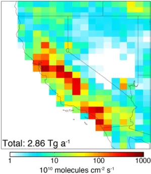
Figure 2 (right) shows optimized correction factors to the EDGAR v4.2 a priori emis-sions from the inversion and Fig. 3 shows the optimized emisemis-sions. The optimized state total emission in California is 2.86±0.21 Tg yr−1, compared with 1.92 Tg yr−1for EDGAR
and 1.51 Tg yr−1 for CARB. The uncertainty on the optimized estimate represents one 5
standard deviation and is provided by the error covariance matrix ˆS computed from Eq. (3). Emissions increase relative to EDGAR v4.2 primarily over the Central Valley, by up to a factor of 4.5. The increase largely follows the pattern of livestock emissions. Emissions decrease over the Los Angeles Basin and the area around Sacramento. Source type allocation is further discussed in Sect. 3.3.
10
Table 2 compares the statewide emissions calculated here and by Santoni et al. (2014). Our state total is larger than their 2.37±0.27 Tg yr−1but this appears to
reflect their use of a lower a priori inventory. When they use the EDGAR v4.2 inventory as a priori in a sensitivity inversion they obtain an optimized emission of 2.8 Tg yr−1, consistent with ours. We conducted sensitivity inversions assuming 50 % and 100 % 15
uncertainties in the EDGAR v4.2 a priori emissions for individual grid squares (instead of 75 % in the standard inversion) and found optimized statewide emissions of 2.59 and 3.10 Tg yr−1, respectively. This illustrates the sensitivity of the optimization to the choice of a priori, although the result that the a priori is too low is robust.
A number of previous studies have used atmospheric observations to estimate 20
methane emissions in the Los Angeles Basin and find values in the range 0.38– 0.6 Tg yr−1 (Table 2). Santoni et al. (2014) estimate a range of 0.29–0.38 Tg yr−1. Our inversion yields an optimized estimate of 0.42±0.08 Tg yr−1for the Los Angeles Basin,
in the range of these previous studies.
The extent to which the inversion can constrain the spatial distribution of emissions in 25
ACPD
14, 4119–4148, 2014Spatially resolving methane emissions
in California
K. J. Wecht et al.
Title Page
Abstract Introduction
Conclusions References
Tables Figures
◭ ◮
◭ ◮
Back Close
Full Screen / Esc
Printer-friendly Version
Interactive Discussion
Discussion
P
a
per
|
D
iscussion
P
a
per
|
Discussion
P
a
per
|
Discuss
ion
P
a
per
that more information is available to constrain the spatial distribution of emissions. In an ideal inversion where allnstate vector elements (emissions in individual grid squares) are fully constrained by the observations,Awould be the identity matrix and we would have DOFS=n.
Figure 4 (top left) shows a map of the diagonal elements ofAin each grid square for 5
the CalNex inversion. Values represent the degrees of freedom associated with each grid square. i.e., the ability of the observations to constrain emissions in that grid square (1=fully, 0=not at all), or in other words the relative contributions of the observations and the a priori in constraining the inverse solution. We find values approaching 1 in the Los Angeles Basin and the San Francisco Bay area, and typically 0.2–0.8 in the Central 10
Valley. Low values are associated with areas that were either not adequately covered by the CalNex aircraft (Fig. 2) or have low a priori emissions (Fig. 1) and thus have little influence on the inversion. Overall our inversion has a total DOFS for California of 12.2, indicating that we can constrain 12 independent pieces of information.
3.3 Attribution to source types
15
Our inversion optimizes methane emissions on a geographical grid without a priori con-sideration of source type. This can be contrasted to the Santoni et al. (2014) inversion, which optimized emissions by source type assuming that the a priori pattern for each source type was correct. Ultimately, our spatial correction factors need to be related to source types in order to guide the improvement of inventories. This can be done by 20
mapping the results onto the a priori source patterns of Fig. 1, with the caveat that the patterns may not be correct.
We conducted the mapping of our optimized emissions to source types by applying the optimized emission correction factors for each grid square (right panel of Fig. 2) to the relative contributions from each major source type in that grid square, as given by 25
emis-ACPD
14, 4119–4148, 2014Spatially resolving methane emissions
in California
K. J. Wecht et al.
Title Page
Abstract Introduction
Conclusions References
Tables Figures
◭ ◮
◭ ◮
Back Close
Full Screen / Esc
Printer-friendly Version
Interactive Discussion
Discussion
P
a
per
|
D
iscussion
P
a
per
|
Discussion
P
a
per
|
Discuss
ion
P
a
per
|
sions in a given grid square. Results in Table 2 show that livestock emissions increase statewide by 92 % relative to EDGAR, landfill/wastewater by 28 %, and gas/oil by 26 %. To examine the degree to which our inversion results can be explained by the pat-terns in the EDGAR a priori inventory, we performed a multiple linear regression (MLR) to fit the inversion corrections in each California grid square of Fig. 3 (n=157) to the 5
a priori spatial patterns from each source type (landfill/wastewater, gas/oil, livestock, other anthropogenic, rice, wetlands, and biofuel;n=7). The MLR best fit has anR2of 0.54, indicating that the a priori source patterns can explain about half of the correc-tion. These patterns are too spatially correlated (e.g., landfill/wastewater and gas/oil in Fig. 1) for the MLR coefficients to provide meaningful attribution to individual source 10
types. The residual not explained by the MLR points to spatial variability in activity rates and emissions factors not accounted for in EDGAR.
We pointed out above the large discrepancies between CARB and EDGAR for dif-ferent source types (Table 2). Our livestock estimate is much higher than EDGAR but agrees with CARB, in contrast to Santoni et al. (2014) who concluded that livestock 15
emissions in CARB are 50 % too low. On the other hand, our emissions from land-fills/wastewater and gas/oil are higher than CARB by factors of 2.7 and 3.6, respec-tively, and are in closer agreement with EDGAR. Rice emissions, although small, are underestimated by a factor of 2–3 in the CARB and EDGAR inventories, consistent with the previous findings of McMillan et al. (2007) and Peischl et al. (2012).
20
4 Utility of current satellites (GOSAT, TES) for constraining california emissions
Satellite observations of atmospheric methane from GOSAT and TES were opera-tional during CalNex and we examine their combined value for constraining emissions from California over that period. GOSAT is in a sun-synchronous polar orbit with an equator overpass local time of∼13:00. It retrieves methane from nadir SWIR spectra
25
near 1.6 µm. Measurements consist of five across-track points separated by∼100 km,
ACPD
14, 4119–4148, 2014Spatially resolving methane emissions
in California
K. J. Wecht et al.
Title Page
Abstract Introduction
Conclusions References
Tables Figures
◭ ◮
◭ ◮
Back Close
Full Screen / Esc
Printer-friendly Version
Interactive Discussion
Discussion
P
a
per
|
D
iscussion
P
a
per
|
Discussion
P
a
per
|
Discuss
ion
P
a
per
use the University of Leicester GOSAT Proxy XCH4 v3.2 data described by Parker et al. (2011) (available from http://www.leos.le.ac.uk/GHG/data/) to populate our obser-vation vectory. These data are for methane column mixing ratiosXCH4 [v/v] retrieved
by the CO2proxy method:
XCH4=
XCO2
ΩCO2
ΩA+aT(ω−ωA)
(5) 5
whereω is the true vertical profile of methane consisting of 20 partial columns, ωA is the a priori profile provided by the TM3 chemical transport model, ΩA is the
corre-sponding a priori column concentration of methane [molecules cm−2],ais an averaging kernel vector that describes the sensitivity as a function of altitude,ΩCO2 is the vertical
column concentration of CO2, andXCO
2 is a modeled column mixing ratio of CO2. The
10
sensitivity characterized byais nearly uniform in the troposphere and decreases with altitude in the stratosphere. The normalization by CO2corrects for aerosol and partial
cloud effects as described by Frankenberg et al. (2006).
TES is in a sun-synchronous polar orbit with an equator overpass local time of ∼
13:45. It retrieves methane from nadir TIR spectra at 7.58–8.55 µm. It makes nadir 15
observations with a pixel resolution of 5.3 km×8.3 km every 182 km along the orbit
track. Successive orbit tracks are separated by about 22◦longitude. We use the most recent V005 Lite product (Worden et al., 2012; http://tes.jpl.nasa.gov/data/). Vertical methane profiles are retrieved as:
ln=ln ˆzA+A′(lnz−lnzA) (6)
20
where ˆz is the retrieved vertical profile vector consisting of mixing ratios on a fixed pressure grid,A′ is the averaging kernel matrix that represents the sensitivity of the retrieved profile to the true profile z, and zA is an a priori profile from the MOZART CTM. TES is mostly sensitive to the middle-upper troposphere and insensitive to the boundary layer. We use it to characterize the free tropospheric background against 25
ACPD
14, 4119–4148, 2014Spatially resolving methane emissions
in California
K. J. Wecht et al.
Title Page
Abstract Introduction
Conclusions References
Tables Figures
◭ ◮
◭ ◮
Back Close
Full Screen / Esc
Printer-friendly Version
Interactive Discussion
Discussion
P
a
per
|
D
iscussion
P
a
per
|
Discussion
P
a
per
|
Discuss
ion
P
a
per
|
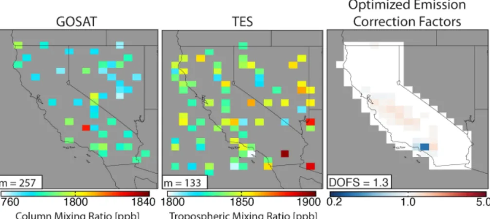
We use GOSAT and TES observations for the CalNex period, 1 May to 22 June 2010, and for the domain (32–42◦N, 125–114◦W), as shown in Fig. 5. There are 257 and 133 GOSAT and TES observations on the GEOS-Chem grid. We subtract biases from GOSAT (−7.5 ppb) and TES (28 ppb) based on validations of Parker et al. (2011) and
Wecht et al. (2012), respectively. We subtract a mean bias of 1.5 ppb from GEOS-Chem 5
based on comparison with TES as measure of the tropospheric background.
Figure 5 (right) shows the optimized correction factors to the a priori EDGAR v4.2 emissions for an inversion using the GOSAT observations. Observational errors for the inversion are determined using the residual error method described above and indicate RSD values in the range 10–12 ppb. The inversion has 1.3 DOFS, compared 10
to 12.2 DOFS for the inversion using the CalNex observations. The correction factors have a pattern similar to those from the CalNex inversion, showing that the constraints from GOSAT on methane emissions are qualitatively consistent with CalNex. However, Central Valley correction factors are driven by just three observations located at the southern end of the Valley, apparent in Fig. 5. Overall, correction factors are much 15
weaker than in the CalNex inversion, reflecting the low DOFS. A map of the degrees of freedom associated with each grid square is shown in Fig. 4 (top, right). 1.1 of the DOFS from GOSAT are for the Los Angeles Basin and the optimization of emissions there should be quantitative: we find 0.31±0.08 Tg yr−1, at the lower end of values in
Table 2. Outside of the Los Angeles Basin the DOFS sum to just 0.2. 20
5 Potential of future satellites (TROPOMI, geostationary)
The TROPOMI satellite instrument (2015 launch) will measure atmospheric methane with far greater coverage than either GOSAT or TES (Table 1). There are in addition several proposals to measure methane from geostationary orbit and the GEO-CAPE in-strument described by Fishman et al. (2012) presents such a possibility. We conducted 25
emis-ACPD
14, 4119–4148, 2014Spatially resolving methane emissions
in California
K. J. Wecht et al.
Title Page
Abstract Introduction
Conclusions References
Tables Figures
◭ ◮
◭ ◮
Back Close
Full Screen / Esc
Printer-friendly Version
Interactive Discussion
Discussion
P
a
per
|
D
iscussion
P
a
per
|
Discussion
P
a
per
|
Discuss
ion
P
a
per
sions in Fig. 3 as the “true” emissions to be retrieved by the inversion, and use these emissions in GEOS-Chem to generate a “true” atmosphere. We sample this “true” at-mosphere with the observation frequency of TROPOMI and GEO-CAPE, apply the corresponding averaging kernels for the instruments, and add random Gaussian noise of the expected magnitude. Instrument specifications are in Table 1. We then conduct 5
an inversion of these synthetic observations exactly as described above, using the a priori emissions described in Sect. 2.2 and shown in Fig. 1, and diagnose the po-tential value of the satellite instruments by their ability to constrain a priori sources as measured by the DOFS. A caveat is that the OSSE uses the same forward model to generate synthetic observations and to invert these observations, and this may lead to 10
overoptimistic inversion results.
We perform OSSEs for the CalNex period of 1 May–22 June 2010 and using syn-thetic observations for the land domain (32–42◦N, 125–114◦W) in the same way as for GOSAT. TROPOMI observations provide complete coverage daily and GEO-CAPE hourly. Both TROPOMI and GEO-CAPE are SWIR instruments and we use a single 15
averaging kernel from GOSAT to generate synthetic observations for both; this is of little consequence as the averaging kernel for SWIR observations is near unity in the troposphere in any case. We randomly remove 80 % of synthetic observations to sim-ulate the effect of cloud cover. Each element of the observation vector y represents the average methane column mixing ratio observed over a GEOS-Chem grid square. 20
When multiple synthetic observations exist in the same 1/2◦
×2/3◦ GEOS-Chem grid
square, we average them into one single observation with square root decrease of the measurement error following the central limit theorem.
Observational error for the OSSE is estimated as the sum of measurement and model error, since the measurements are dense enough that representation error can 25
be neglected. We specify the model error standard deviation to be 12 ppb, a conser-vative estimate based on the observational error for GOSAT. Measurement error (Ta-ble 1) and model error are added in quadrature to populate the diagonal of SO and
ACPD
14, 4119–4148, 2014Spatially resolving methane emissions
in California
K. J. Wecht et al.
Title Page
Abstract Introduction
Conclusions References
Tables Figures
◭ ◮
◭ ◮
Back Close
Full Screen / Esc
Printer-friendly Version
Interactive Discussion
Discussion
P
a
per
|
D
iscussion
P
a
per
|
Discussion
P
a
per
|
Discuss
ion
P
a
per
|
the averaging of the measurements over GEOS-Chem grid squares described above. The a priori error covariance matrix is populated in the same way as above. We assume no background bias in the model or observations as this could be corrected through other observations such as a TIR instrument (e.g., TES for GOSAT) or by iterative adjustment of emissions and boundary conditions in the inversion (Wecht et al., 2013). 5
Figure 4 (bottom) summarizes the OSSE results. The TROPOMI inversion has 10.5 DOFS (Fig. 4, bottom, left), comparable to the CalNex inversion (12.2 DOFS), and it accurately captures the spatial pattern of a priori emission errors. Optimized statewide emissions are 2.60 Tg yr−1, compared with 2.86 Tg yr−1 from the “true” emissions. We conclude that TROPOMI may perform just as well as a dedicated aircraft campaign 10
(CalNex), and is thus superbly positioned to constrain emissions at the state level. The GEO-CAPE inversion has 26.5 DOFS (Fig. 4, bottom, right), much higher than Cal-Nex and TROPOMI, reflecting the greater density of observations. Optimized statewide emissions are 2.79 Tg yr−1
, close to the “true” emissions of 2.86 Tg yr−1
. This reveals the considerable potential of geostationary observations for monitoring methane emis-15
sions on fine scales.
6 Conclusions
We applied an inverse modeling system based on the GEOS-Chem Eulerian chemical transport model (CTM) to optimize methane emissions from Califonia with 1/2◦
×2/3◦
horizontal resolution using observations from the May–June 2010 CalNex aircraft cam-20
paign. The system is designed to optimize emissions on the continental scale us-ing satellite observations (Wecht et al., 2014) and here we evaluated its potential to constrain the spatial distribution of emissions at the state level. We compared the constraints achievable with the CalNex aircraft observations to those achievable from current (GOSAT, TES) and future (TROPOMI, geostationary) satellite observations of 25
ACPD
14, 4119–4148, 2014Spatially resolving methane emissions
in California
K. J. Wecht et al.
Title Page
Abstract Introduction
Conclusions References
Tables Figures
◭ ◮
◭ ◮
Back Close
Full Screen / Esc
Printer-friendly Version
Interactive Discussion
Discussion
P
a
per
|
D
iscussion
P
a
per
|
Discussion
P
a
per
|
Discuss
ion
P
a
per
observations (Santoni et al., 2013), thus providing a perspective on the use of different inversion methodologies. Because the inversion was conducted over a limited spatial domain, we could obtain analytical solutions with full error characterization to compare the different observing systems.
Our inversion of CalNex observations yields a best estimate of 2.86±0.21 Tg yr−1
5
for total California emissions, compared to 1.92 Tg yr−1 in the EDGAR v4.2 inventory used as a priori for the inversion, 1.51 Tg yr−1 in the California Air Resources Board (CARB) inventory used as basis to regulate greenhouse gas emissions in California, and 2.37±0.27 Tg yr−1in the Santoni et al. (2014) inversion. Our results are consistent
with Santoni et al. (2014) considering that they used a lower a priori emission estimate 10
for their inversion. An important distinction between the two inversions is that we op-timize emissions geographically in 157 grid squares whereas they opop-timize emissions for 8 source types. Error statistics on our inversion indicates that it provides 12 inde-pendent pieces of information (measured by degrees of freedom for signal or DOFS). We have particularly strong constraints on emissions in the Los Angeles Basin where 15
our emission estimate (0.42±0.08 Tg yr−1) is consistent with previous studies.
The CARB and EDGAR v4.2 emission inventories show factor of 2 differences between each other in their state total estimates of emissions from livestock, land-fills/wastewater, and gas/oil. Our results provide guidance for resolving these discrep-ancies. Mapping our optimized estimate of the spatial distribution of California methane 20
emissions onto individual source types indicates a state total livestock emission of 0.87 Tg yr−1, in close agreement with CARB but much higher than EDGAR and lower than the 1.29 Tg yr−1 estimate of Santoni et al. (2014). On the other hand, our best estimate of emissions from landfills/wastewater (1.05 Tg yr−1) and gas/oil (0.64 Tg yr−1) is 20 % higher than EDGAR but much higher than CARB or Santoni et al. (2014). Our 25
ACPD
14, 4119–4148, 2014Spatially resolving methane emissions
in California
K. J. Wecht et al.
Title Page
Abstract Introduction
Conclusions References
Tables Figures
◭ ◮
◭ ◮
Back Close
Full Screen / Esc
Printer-friendly Version
Interactive Discussion
Discussion
P
a
per
|
D
iscussion
P
a
per
|
Discussion
P
a
per
|
Discuss
ion
P
a
per
|
manure management practices) and activity rates (e.g. landfill locations and gas/oil production).
We find that current satellite observations of methane from GOSAT and TES are too sparse to quantitatively constrain California emissions. TES is only useful for con-straining the free tropospheric background. GOSAT provides quantitative constraints 5
on emissions in the Los Angeles Basin (0.31±0.08 Tg yr−1) but not elsewhere.
How-ever, the qualitative corrections to a priori emissions from the GOSAT observations across the state are consistent with those from the CalNex observations. They consis-tently point to a large underestimate of livestock emissions in the EDGAR v4.2 inven-tory. In the absence of a dedicated aircraft study such as CalNex, GOSAT can be useful 10
as a qualitative indicator of biases in methane emission inventories. Furthermore, as-similating current satellite observations over larger spatiotemporal scales may improve their ability to constrain emissions.
The TROPOMI satellite instrument to be launched in 2015 has considerable potential for improving our capability to monitor methane emissions from space. TROPOMI will 15
provide global daily coverage of methane columns with 7 km×7 km nadir resolution.
We find in an observation system simulation experiment (OSSE) that the observing power of TROPOMI for constraining methane emissions in California will be compa-rable to that of the CalNex aircraft campaign. Geostationary observations of methane proposed for the coming decade have even more potential for constraining methane 20
emissions. These satellite measurements will provide monitoring, reporting, and veri-fication (MRV) for the development of methane emission control strategies in the con-text of climate policy. This will be particularly important in a world of rapidly changing methane emissions from natural gas exploitation, hydrofracking, and agricultural man-agement practices.
25
Acknowledgements. This work was supported by the NASA Carbon Monitoring System (CMS),
ACPD
14, 4119–4148, 2014Spatially resolving methane emissions
in California
K. J. Wecht et al.
Title Page
Abstract Introduction
Conclusions References
Tables Figures
◭ ◮
◭ ◮
Back Close
Full Screen / Esc
Printer-friendly Version
Interactive Discussion
Discussion
P
a
per
|
D
iscussion
P
a
per
|
Discussion
P
a
per
|
Discuss
ion
P
a
per
supported by the UK National Centre for Earth Observation and the European Space Agency Climate Change Initiative.
References
Allen, D., Pickering, K., Duncan, B., and Damon, M.: Impact of lightning NO emissions on North American photochemistry as determined using the Global Modeling Initiative (GMI) model, J.
5
Geophys. Res., 115, D22301, doi:10.1029/2010JD014062, 2010.
Butz, A., Galli, A., Hasekamp, O., Landgraf, J., Tol, P., and Aben, I.: TROPOMI aboard Precursor Sentinel-5 Precursor: prospective performance of CH4retrievals for aerosol and cirrus loaded atmospheres, Remote Sens. Environ., 120, 267–276, doi:10.1016/j.rse.2011.05.030, 2012. California Air Resources Board: California Greenhouse Gas Emission Inventory: 2000–2009,
10
available at: http://www.arb.ca.gov/cc/inventory/pubs/reports/ghg_inventory_00-09_report. pdf (last access: 4 February 2014), 2011.
California Air Resources Board: Climate Change Scoping Plan First Update: Discussion Draft for Public Review and Comment, available at: http://www.arb.ca.gov/cc/scopingplan/2013_ update/discussion_draft.pdf (last access: 4 February 2014), 2013.
15
Committee on Methods for Estimating Greenhouse Gas Emissions: Verifying greenhouse gas emissions: methods to support international climate agreements, National Research Council, Natl. Acad. Press, Washington, DC, USA, 2010.
Considine, D. B., Logan, J. A., and Olsen, M. A.: Evaluation of near-tropopause ozone dis-tributions in the Global Modeling Initiative combined stratosphere/troposphere model with
20
ozonesonde data, Atmos. Chem. Phys., 8, 2365–2385, doi:10.5194/acp-8-2365-2008, 2008. Crevoisier, C., Nobileau, D., Armante, R., Crépeau, L., Machida, T., Sawa, Y., Matsueda, H.,
Schuck, T., Thonat, T., Pernin, J., Scott, N. A., and Chédin, A.: The 2007–2011 evolution of tropical methane in the mid-troposphere as seen from space by MetOp-A/IASI, Atmos. Chem. Phys., 13, 4279–4289, doi:10.5194/acp-13-4279-2013, 2013.
25
European Commission, Joint Research Centre (JRC)/Netherlands Environmental Assessment Agency (PBL): Emission Database for Global Atmospheric Research (EDGAR), release ver-sion 4.0, available at: http://edgar.jrc.ec.europa.eu (last access: 4 February 2014), 2009. Fast, J. D., Gustafson Jr., W. I., Berg, L. K., Shaw, W. J., Pekour, M., Shrivastava, M.,
Barnard, J. C., Ferrare, R. A., Hostetler, C. A., Hair, J. A., Erickson, M., Jobson, B. T.,
ACPD
14, 4119–4148, 2014Spatially resolving methane emissions
in California
K. J. Wecht et al.
Title Page
Abstract Introduction
Conclusions References
Tables Figures
◭ ◮
◭ ◮
Back Close
Full Screen / Esc
Printer-friendly Version
Interactive Discussion
Discussion
P
a
per
|
D
iscussion
P
a
per
|
Discussion
P
a
per
|
Discuss
ion
P
a
per
|
Flowers, B., Dubey, M. K., Springston, S., Pierce, R. B., Dolislager, L., Pederson, J., and Zaveri, R. A.: Transport and mixing patterns over Central California during the carbona-ceous aerosol and radiative effects study (CARES), Atmos. Chem. Phys., 12, 1759–1783, doi:10.5194/acp-12-1759-2012, 2012.
Fishman, J., Iraci, L. T., Al-Saadi, J., Chance, K., Chavez, F., Chin, M., Coble, P., Davis, C.,
5
DiGiacomo, P. M., Edwards, D., Eldering, A., Goes, J., Herman, J., Hu, C., Jacob, D. J., Jor-dan, C., Kawa, S. R., Key, R., Liu, X., Lohrenz, S., Mannino, A., Natraj, V., Neil, D., Neu, J., Newchurch, M., Pickering, K., Salisbury, J., Sosik, H., Subramaniam, A., Tzortziou, M., Wang, J., and Wang, M.: The United States’ next generation of atmospheric composition and coastal ecosystem measurements: NASA’s geostationary coastal and air pollution events
10
(GEO-CAPE) mission, B. Am. Meteorol. Soc., 93, 1547–1566, 2012.
Frankenberg, C., Meirink, J. F., Bergamaschi, P., Goede, A. P. H., Heimann, M., Körner, S., Platt, U., van Weele, M., and Wagner, T.: Satellite chartography of atmospheric methane from SCIAMACHY on board ENVISAT: analysis of the years 2003 and 2004, J. Geophys. Res., 111, D07303, doi:10.1029/2005JD006235, 2006.
15
Frankenberg, C., Aben, I., Bergamaschi, P., Dlugokencky, E. J., van Hees, R., Houweling, S., van der Meer, P., Snel, R., and Tol, P.: Global column-averaged methane mixing ratios from 2003 to 2009 as derived from SCIAMACHY: trends and variability, J. Geophys. Res., 116, D02304, doi:10.1029/2010JD014849, 2011.
Fung, I., John, J., Lerner, J., Matthews, E., Prather, M., Steele, L. P., and Fraser, P. J.:
Three-20
dimensional model synthesis of the global methane cycle, J. Geophys. Res., 96, 13033– 13065, 1991.
Heald, C., Jacob, D., Jones, D., Palmer, P., Logan, J., Streets, D., Sachse, G., Gille, J., Hoff -man, R., and Nehrkorn, T.: Comparative inverse analysis of satellite (MOPITT) and aircraft (TRACE-P) observations to estimate Asian sources of carbon monoxide, J. Geophys.
Res.-25
Atmos., 109, D23306, doi:10.1029/2004JD005185, 2004.
Hsu, Y.-K., VanCuren, T., Park, S., Jakober, C., Herner, J., FitzGibbon, M., Blake, D. R., and Par-rish, D. D.: Methane emission inventory verification in southern California, Atmos. Environ., 44, 1–7, 2010.
Jeong, S., Zhao, C., Andrews, A. E., Bianco, L., Wilczak, J. M., and Fischer, M. L.:
Sea-30
ACPD
14, 4119–4148, 2014Spatially resolving methane emissions
in California
K. J. Wecht et al.
Title Page
Abstract Introduction
Conclusions References
Tables Figures
◭ ◮
◭ ◮
Back Close
Full Screen / Esc
Printer-friendly Version
Interactive Discussion
Discussion
P
a
per
|
D
iscussion
P
a
per
|
Discussion
P
a
per
|
Discuss
ion
P
a
per
Kaplan, J. O.: Wetlands at the Last Glacial Maximum: distribution and methane emissions, Geophys. Res. Lett., 29, 1079, doi:10.1029/2001GL013366, 2002.
Kort, E. A., Wofsy, S. C., Daube, B. C., Diao, M., Elkis, J. W., Gao, R. S., Hintsa, E. J., Hurst, D. F., Jimenez, R., Moore, F. L., Spackman, J. R., and Zondlo, M. A.: Atmospheric observations of Arctic Ocean methane emissions up to 82◦ north, Nat. Geosci., 5, 318–321,
5
doi:10.1038/NGEO1452, 2012.
McMillan, A. M. S., Goulden, M. L., and Tyler, S. C.: Stoichiometry of CH4 and CO2 flux in a California rice paddy, J. Geophys. Res., 112, G01008, doi:10.1029/2006JG000198, 2007. Mu, M., Randerson, J. T., van der Werf, G. R., Giglio, L., Kasibhatla, P., Morton, D., Collatz, G. J.,
DeFries, R. S., Hyer, E. J., Prins, E. M., Griffith, D. W. T., Wunch, D., Toon, G. C.,
Sher-10
lock, V., and Wennberg, P. O.: Daily and 3 hourly variability in global fire emissions and con-sequences for atmospheric model predictions of carbon monoxide, J. Geophys. Res.-Atmos, 116, D24303, doi:10.1029/2011JD016245, 2010.
Park, R. J., Jacob, D. J., Field, B. D., Yantosca, R. M., and Chin, M.: Natural and transboundary pollution influences on sulfate-nitrate-ammonium aerosols in the United States: implications
15
for policy, J. Geophys. Res., 109, D15204, doi:10.1029/2003JD004473, 2004.
Parker, R., Boesch, H., Cogan, A., Fraser, A., Feng, L., Palmer, P. I., Messerschmidt, J., Deutscher, N., Griffith, D. W., Notholt, J., Wennberg, P. O., and Wunch, D.: Methane observa-tions from the Greenhouse Gases Observing SATellite: comparison to ground-based TCCON data and model calculations, Geophys. Res. Lett., 38, L15807, doi:10.1029/2011GL047871,
20
2011.
Peischl, J., Ryerson, T. B., Holloway, J. S., Trainer, M., Andrews, A. E., Atlas, E. L., Blake, D. R., Daube, B. C., Dlugokencky, E. J., Fischer, M. L., Goldstein, A. H., Guha, A., Karl, T., Kofler, J., Kosciuch, E., Misztal, P. K., Perring, A. E., Pollack, I. B., Santoni, G. W., Schwarz, J. P., Spackman, J. R., Wofsy, S. C., and Parrish, D. D.: Airborne observations of methane
emis-25
sions from rice cultivation in the Sacramento Valley of California, J. Geophys. Res., 117, D00V25, doi:10.1029/2012JD017994, 2012.
Rodgers, C. D.: Inverse Methods for Atmospheric Sounding, World Scientific Publishing Co. Pte. Ltd, Tokyo, 2000.
Santoni, G. W., Xiang, B., Kort, E. A., Daubel, B. C., Andrews, A. E., Sweeney, C., Wecht, K. J.,
30
de-ACPD
14, 4119–4148, 2014Spatially resolving methane emissions
in California
K. J. Wecht et al.
Title Page
Abstract Introduction
Conclusions References
Tables Figures
◭ ◮
◭ ◮
Back Close
Full Screen / Esc
Printer-friendly Version
Interactive Discussion
Discussion
P
a
per
|
D
iscussion
P
a
per
|
Discussion
P
a
per
|
Discuss
ion
P
a
per
|
rived from CalNex P-3 Aircraft Observations and a Lagrangian transport model, J. Geophys. Res., submitted, 2014.
Santoni, G. W., Daube, B. C., Kort, E. A., Jiménez, R., Park, S., Pittman, J. V., Gottlieb, E., Xiang, B., Zahniser, M. S., Nelson, D. D., McManus, J. B., Peischl, J., Ryerson, T. B., Hol-loway, J. S., Andrews, A. E., Sweeney, C., Hall, B. D., Hintsa, E. J., Moore, F. L., Elkins, J. W.,
5
Hurst, D. F., Stephens, B. B., Bent, J. D., and Wofsy, S. C.: Evaluation of the Airborne Quan-tum Cascade Laser Spectrometer (QCLS) measurements of the carbon and greenhouse gas suite – CO2, CH4, N2O, and CO – during the CalNex and HIPPO campaigns, Atmos. Meas. Tech. Discuss., 6, 9689–9734, doi:10.5194/amtd-6-9689-2013, 2013.
Schepers, D., Guerlet, S., Butz, A., Landgraf, J., Frankenberg, C., Hasekamp, O., Blavier,
J.-10
F., Deutscher, N. M., Griffith, D. W. T., Hase, F., Kyro, E., Morino, I., Sherlock, V., Suss-mann, R., and Aben, I.: Methane retrievals from Greenhouse Gases Observing Satellite (GOSAT) shortwave infrared measurements: performance comparison of proxy and physics retrieval algorithms, J. Geophys. Res., 117, D10307, doi:10.1029/2012JD017549, 2012. Singh, H. B., Brune, W. H., Crawford, J. H., and Jacob, D. J.: Overview of the summer 2004
In-15
tercontinental Chemical Transport Experiment-North America (INTEX-A), J. Geophys. Res., 111, D24S01, doi:10.1029/2006JD007905, 2012.
United States Environmental Protection Agency (EPA): Inventory of US Greenhouse Gas Emissions and Sinks: 1990–2011-Annexes, available at: http://www.epa.gov/climatechange/ Downloads/ghgemissions/US-GHG-Inventory-2013-Main-Text.pdf (last access: 4 February
20
2014), 2013.
van der Werf, G. R., Randerson, J. T., Giglio, L., Collatz, G. J., Mu, M., Kasibhatla, P. S., Mor-ton, D. C., DeFries, R. S., Jin, Y., and van Leeuwen, T. T.: Global fire emissions and the contribution of deforestation, savanna, forest, agricultural, and peat fires (1997–2009), At-mos. Chem. Phys., 10, 11707–11735, doi:10.5194/acp-10-11707-2010, 2010.
25
Veefkind, J. P., Aben, I., McMullan, K., Forster, H., de Vries, J., Otter, G., Claas, J., Eskes, H. J., de Haan, J. F., Kleipool, Q., van Weele, M., Hasekamp, O., Hoogeveen, R., Landgraf, J., Snel, R., Tol, P., Ingmann, P., Voors, R., Kruizinga, B., Vink, R., Visser, H., and Levelt, P. F.: TROPOMI on the ESA Sentinel-5 Precursor: a GMES mission for global observations of the atmospheric composition for climate, air quality and ozone layer applications, Remote Sens.
30
Environ., 120, 70–83, 2012.
ACPD
14, 4119–4148, 2014Spatially resolving methane emissions
in California
K. J. Wecht et al.
Title Page
Abstract Introduction
Conclusions References
Tables Figures
◭ ◮
◭ ◮
Back Close
Full Screen / Esc
Printer-friendly Version
Interactive Discussion
Discussion
P
a
per
|
D
iscussion
P
a
per
|
Discussion
P
a
per
|
Discuss
ion
P
a
per
implications for inverse modeling of methane sources, Atmos. Chem. Phys., 12, 1823–1832, doi:10.5194/acp-12-1823-2012, 2012.
Wecht, K. J., Jacob, D. J., Frankenberg, C., Blake, D. R., and Jiang, Z.: Mapping of North Amer-ican methane emissions with high spatial resolution by inversion of SCIAMACHY satellite data, submitted, 2014.
5
Wennberg, P. O., Mui, W., Wunch, D., Kort, E. A., Blake, D. R., Atlas, E. L., Santoni, G. W., Wofsy, S. C., Diskin, G. S., Jeong, S., and Fischer, M. L.: On the sources of methane to the Los Angeles atmosphere, Environ. Sci. Technol., 46, 9282–9289, 2012.
Worden, J. R., Jiang, Z., Jones, D. B. A., Alvarado, M., Bowman, K., Frankenberg, C., Kort, E. A., Kulawik, S. S., Lee, M., Liu, J., Payne, V., Wecht, K., and Worden, H.: El Niño, the 2006
10
Indonesian peat fires, and the distribution of atmospheric methane, Geophys. Res. Lett., 40, 4938–4943, doi:10.1002/grl.50937, 2008.
Worden, J., Kulawik, S., Frankenberg, C., Payne, V., Bowman, K., Cady-Peirara, K., Wecht, K., Lee, J.-E., and Noone, D.: Profiles of CH4, HDO, H2O, and N2O with improved lower tro-pospheric vertical resolution from Aura TES radiances, Atmos. Meas. Tech., 5, 397–411,
15
doi:10.5194/amt-5-397-2012, 2012.
Wunch, D., Wennberg, P. O., Toon, G. C., Keppel-Aleks, G., and Yavin, Y. G.: Emissions of greenhouse gases from a North American megacity, Geophys. Res. Lett., 36, L15810, doi:10.1029/2009GL039825, 2009.
Xiong, X., Barnet, C. D., Maddy, E., Sweeney, C., Liu, X., Zhou, L., and Goldberg, M.:
Character-20
ization and validation of methane products from the Atmospheric Infrared Sounder (AIRS), J. Geophys. Res., 113, G00A01, doi:10.1029/2007JG000500, 2008.
Xiong, X., Barnet, C., Maddy, E. S., Gambacorta, A., King, T. S., and Wofsy, S. C.: Mid-upper tropospheric methane retrieval from IASI and its validation, Atmos. Meas. Tech., 6, 2255– 2265, doi:10.5194/amt-6-2255-2013, 2013.
25
ACPD
14, 4119–4148, 2014Spatially resolving methane emissions
in California
K. J. Wecht et al.
Title Page
Abstract Introduction
Conclusions References
Tables Figures
◭ ◮
◭ ◮
Back Close
Full Screen / Esc
Printer-friendly Version
Interactive Discussion
Discussion
P
a
per
|
D
iscussion
P
a
per
|
Discussion
P
a
per
|
Discuss
ion
P
a
per
|
Table 1.Satellite observations of methane.
Wavelength Return Pixel DOFS for
Instrument range Launch time resolution Precision California Reference (days)a (km2)b emissionsc
Globald
SCIAMACHY SWIR 2002e 6 30×60 1.5 % Frankenberg et al. (2011) AIRS TIR 2002 0.5 45×45 1.5 % Xiong et al. (2008) TES TIR 2004f 16 5×8f 1 % ∼0 Worden et al. (2012) IASI TIR 2007 0.5 50×50 1.2 % Xiong et al. (2013);
Crevoisier et al. (2013) GOSAT SWIR 2009 3 ∼10×10g 0.6 % 1.3 Parker et al. (2011);
Schepers et al. (2012) TROPOMI SWIR 2015 1 7×7 0.6 % 10.5 Veefkind et al. (2012);
Butz et al. (2012) Geostationary
GEO-CAPEh SWIR ∼2020i Hourly 4×4 1.1 % 26.5 Fishman et al. (2012) aFull global coverage except for TES and GOSAT (see footnotes f and g).
bFor nadir view.
cThe Degrees of Freedom for Signal (DOFS) measures the capability of the satellite observations for the CalNex period (1 May–22 June 2010) to constrain the spatial distribution of emissions in California. Values are shown only for satellite instruments used in this work. Results for TROPOMI and GEO-CAPE are from Observation System Simulation Experiments (OSSEs). The CalNex aircraft observations have DOFS of 12.2. See text for details.
dFrom polar sun-synchronous low-elevation orbit.
eTerminated in 2012; methane retrieval quality degraded after 2005.
fTES measurements are limited to the orbit tracks. Regular global surveys were terminated at the end of 2011. gGOSAT takes measurements at 5 across-track points separated by 100 km, each with a ground footprint diameter of 10 km.
ACPD
14, 4119–4148, 2014Spatially resolving methane emissions
in California
K. J. Wecht et al.
Title Page
Abstract Introduction
Conclusions References
Tables Figures
◭ ◮
◭ ◮
Back Close
Full Screen / Esc
Printer-friendly Version
Interactive Discussion
Discussion
P
a
per
|
D
iscussion
P
a
per
|
Discussion
P
a
per
|
Discuss
ion
P
a
per
Table 2.Methane emissions in Californiaa.
CARB EDGAR Santoni This Other v4.2b et al. (2014)c studyd studiese
State Total 1.51 1.92 2.37±0.27 2.86±0.21 Landfills/wastewaterf 0.39 0.82 0.42g 1.05 Gas/oil 0.18 0.51 footnotec 0.64 Livestock 0.86 0.46 1.29 0.87
Rice 0.027 0.033 0.069 0.08 0.078–0.093h Otheri 0.05 0.10 footnotec 0.13
Naturalj 0.08
Los Angeles Basin 0.54 0.28–0.39 0.42±0.08 0.6±0.1l 0.31±0.08k 0.38±0.1m
0.44±0.15n 0.41±0.04o
aUnits are Tg yr−1. Estimates from the CARB and EDGAR v4.2 inventories are compared to inversion results from this work and other studies. Values are for 2010 unless otherwise noted. bFor 2008, the latest year available.
cLagrangian inversion using CalNex observations and resolving 8 source types/regions. They give a total emission estimate of 0.59 Tg yr−1from the sum of wastewater, gas/oil, and other sources without a further source breakdown.
dInversion at 1 /2◦
×2/3◦resolution using CalNex observations unless otherwise indicated; source
type attribution is inferred by mapping optimized emissions to the EDGAR source type distributions. eEstimates constrained by atmospheric observations from surface or aircraft.
fThese two sources are combined here because of the similarity of their geographical distributions in EDGAR v4.2. Landfills account for 80 % of this combined source according to both CARB and EDGAR v4.2.
gLandfills only.
hMcMillan et al. (2007), Peischl et al. (2012) iIncluding biofuels and other minor sources. jIncluding wetlands, termites, and open fires.
kFrom inversion of GOSAT observations during CalNex. lWunch et al. (2009) estimate for 2007–2008.
mHsu et al. (2010) estimate for 2007–2008.
ACPD
14, 4119–4148, 2014Spatially resolving methane emissions
in California
K. J. Wecht et al.
Title Page
Abstract Introduction
Conclusions References
Tables Figures
◭ ◮
◭ ◮
Back Close
Full Screen / Esc
Printer-friendly Version
Interactive Discussion
Discussion
P
a
per
|
D
iscussion
P
a
per
|
Discussion
P
a
per
|
Discuss
ion
P
a
per
|
Fig. 1.EDGAR v4.2 methane emissions for 2008 used as a priori for our inversion. Panels
ACPD
14, 4119–4148, 2014Spatially resolving methane emissions
in California
K. J. Wecht et al.
Title Page
Abstract Introduction
Conclusions References
Tables Figures
◭ ◮
◭ ◮
Back Close
Full Screen / Esc
Printer-friendly Version
Interactive Discussion
Discussion
P
a
per
|
D
iscussion
P
a
per
|
Discussion
P
a
per
|
Discuss
ion
P
a
per
Fig. 2.Mean methane concentrations below 2 km altitude during CalNex (May–June 2010).
Aircraft observations averaged on the 1/2◦
×2/3◦GEOS-Chem grid (left) are compared to the
ACPD
14, 4119–4148, 2014Spatially resolving methane emissions
in California
K. J. Wecht et al.
Title Page
Abstract Introduction
Conclusions References
Tables Figures
◭ ◮
◭ ◮
Back Close
Full Screen / Esc
Printer-friendly Version
Interactive Discussion
Discussion
P
a
per
|
D
iscussion
P
a
per
|
Discussion
P
a
per
|
Discuss
ion
P
a
per
|
Fig. 3.Optimized methane emissions from our inversion using CalNex observations. Total
ACPD
14, 4119–4148, 2014Spatially resolving methane emissions
in California
K. J. Wecht et al.
Title Page
Abstract Introduction
Conclusions References
Tables Figures
◭ ◮
◭ ◮
Back Close
Full Screen / Esc
Printer-friendly Version
Interactive Discussion
Discussion
P
a
per
|
D
iscussion
P
a
per
|
Discussion
P
a
per
|
Discuss
ion
P
a
per
Fig. 4.Degrees of freedom in each grid square from our inversions using CalNex (top, left) and
ACPD
14, 4119–4148, 2014Spatially resolving methane emissions
in California
K. J. Wecht et al.
Title Page
Abstract Introduction
Conclusions References
Tables Figures
◭ ◮
◭ ◮
Back Close
Full Screen / Esc
Printer-friendly Version
Interactive Discussion
Discussion
P
a
per
|
D
iscussion
P
a
per
|
Discussion
P
a
per
|
Discuss
ion
P
a
per
|
Fig. 5.Mean methane mixing ratios measured by GOSAT (left) and TES (center) for the CalNex