Rakenteiden Mekaniikka (Journal of Structural Mechanics) Vol. 46, No 4, 2013, pp. 116 – 130
On the solution of non-linear diffusion equation
Reijo Kouhia
Summary. Solution of the diffusion equation is usually performed with the finite element discretization for the spatial elliptic part of the equation and the time dependency is integrated via some difference scheme, often the trapezoidal rule (Crank-Nicolson) or the unconditionally stable semi-implicit two-step algorithm of Lees. A common procedure is to use Picard’s iteration with the trapezoidal rule. However, in highly non-linear problems the convergence of Picard’s iteration is untolerably slow. A simple remedy is to use consistent linearization and Newton’s method. For a certain class of non-linear constitutive models the consistent Jacobian matrix is unsymmetric. This paper discusses the use of the symmetric part of the Jacobian matrix and a combined Newton-type iteration scheme. Numerical results of highly non-linear diffusion problems are shown. Also a note concerning temporal discretization is given.
Key words: non-linear diffusion equation, finite elements, Newton’s method
Introduction
Many diffusive phenomena are governed by the balance equation
−∇ ·q+s=cu,˙ (1)
where q is the flux vector, which is related to the gradient of the quantity u by the constitutive law
q=−D(u,g)g, g =∇u. (2) Time derivatives are indicated by superimposed dots (∂u/∂t= ˙u). Equations (1) and (2) form a system which can be used to describe many diffusive physical phenomena, e.g. heat conduction, seepage flow, electric fields and frictionless incompressible irrotational flow. In the case of heat conduction u stands for temperature and s, c,q are the heat source, the heat capacity and the heat flux, respectively. In certain applications the source terms
can depend on the solutionuand the resulting equation is known as the diffusion-reaction equation.
In the case of heat transfer the boundary conditions can be either prescribed temper-ature
u=uS, on the boundary part Su, (3)
specified heat flux
q·n=−qS, on the boundary part Sq, (4) a convection boundary condition
or a radiation boundary condition
q·n=σεu4−βqr, on the boundary part Sr, (6) whereh is the convection coefficient, uex convective exchange temperature,σ the Stefan-Bolzmann constant,εthe surface emission coefficient,βthe surface absorption coefficient, and qr the incident radiant heat flow per unit surface are, respectively. For transient problems also an initial temperature field should be specified.
After finite element semidiscretization, the balance equation (1) takes the form C ˙u=f(t,u), (7) in which Cis the Gram matrix− in heat transfer analysis the capacitance matrix− and f denotes the unbalance between the given sources and the internal nodal ‘fluxes’ r, i.e.
f =s−r. (8)
The Gram matrix, the internal nodal flux and the source vectors are computed from the element contributions
Ce = Z
Ve
cNTNdV , r(e)= Z
V(e)
BTqdV , s(e)= Z
V(e)
NTsdV , (9) whereB is the matrix of discretized gradient operator andNis the row matrix containing the finite element interpolation functions. In rectangular Cartesian coordinate system the discrete gradient matrix has the form
B=
N,x
N,y
N,z
. (10)
Further details in the finite element solution of diffusion equation can be found in the excellent textbooks [17, 26].
If the temporal discretization is performed by the one-step one-parameter method un+α= (1−α)un+αun+1, (11) and the time derivative u˙n+α is approximated as
˙ un+α ≈
un+1−un
∆t , (12)
then from (7) the fully discretized equation system is obtained 1
α∆tC(un+α−un)−f(tn+α,un+α) =0. (13)
order accurate. In linear autonomous cases the midpoint scheme is identical with the standard trapezoidal rule.
The trapezoidal rule has no algorithmic damping. This produces spurious oscillations if the data is not smooth. A simple remedy for suppressing these oscillations is to use for the few first steps the implicit backward Euler scheme and then switch to the second order accurate midpoint rule [19, 25]. This has no effect on the long term accuracy.
In order to solve the non-linear equation system (13) a Newton-type linearization step is utilized and the resulting equation, at a certain step n+ 1 and iteration i, is the following:
1
α∆tC i+Ki
δui+1 =f(tn+α,ui
n+α)−
1
α∆tC
i∆ui, (14)
where
Ki =−∂f
∂u
uin+α
(15) is the Jacobian matrix1, and the iterative and incremental steps are defined by
δui+1 =ui+1
n+α−u i
n+α, ∆u i
=uin+α−un, thus uin+1+α =un+∆ui+δui+1. (16)
The Jacobian matrix consists of several parts:
Ki =Ki0+Kiu+Kig+Kis+Kir, (17) where K0 is the linear part, Ku and Kg come from the u and g dependencies of the
constitutive equation (2), Kr from the non-linear radiation boundary condition and Ks
from theu dependent source term. They are assembled from the element matrices K(0e)i =
Z
V(e)
BTDiBdV , Di =D(ui,gi), (18)
K(ue)i = Z
V(e)
BTGidV , Gi = ∂D
∂u
ui,
gi
!
giN, (19)
K(ge)i = Z
V(e)
BTDigBdV , Dig = ∂D
∂g ui,
gi
!
gi, (20)
K(se)i = Z
V(e)
∂s¯
∂uN TN
dV , (21)
K(re)i = Z
Sr(e)
Ci rN
TNdS, (22)
where Cr is a temperature dependent term containing the radiation and emission coef-ficients of the radiating surface. All matrices, except Ku, are symmetric. Dependency
of the constitutive matrix D on u is common in many physical problems. However, the unsymmetric part is usually neglected in the solution of equation (14), which causes con-vergence problems in highly non-linear cases.
Consequenses of the loss of symmetry seems to be purely practical. Memory re-quirements will double and are thus very high for large three dimensional computations, especially if a direct linear equation solver is used. Also iterative solvers for unsymmet-ric linear equations are not as robust as symmetunsymmet-ric ones, even though a lot of effort to increase their reliability has been paid during the last decades [28, 21, 29].
1
Since the unsymmetric part of the Jacobian matrix resembles the convective part of the coefficient matrix in the diffusion-convection equation, one would expect numerical instabilities if standard finite-element approximation is used. However, numerical oscilla-tions were not observed in the numerical experiments. Additional discussion can also be found in the section on numerical examples.
In this paper standard Galerkin finite element technique is used. Good introduction to the selection of optimal weighting functions can be found in Refs. [6, 7]. An interesting recent Hybrid-Trefftz finite element method for the thermal analysis of functionaly graded materials is given in Ref. [8]. Weak Galerkin finite element method is considered in Ref. [18].
In order to avoid the use of an unsymmetric iteration matrix some modified iteration schemes are studied. First, quasi-Newton techniques are shortly described. Secondly, a possible iteration scheme for the solution of the unsymmetric linear equation system is described. It utilizes the Neumann series and element by element type matrix-vector multiplication of the unsymmetric part of the Jacobian matrix. Finally, a combined Newton iteration process is described.
Quasi-Newton techniques
Basic properties
A class of inexact Newton algorithms called quasi-Newton (or variable metric, variance, secant, update or modification methods) have been developed in order to speed up the convergence of the modified Newton method2 and which could be more efficient than the true Newton-Raphson scheme. The basic idea of these methods is to develope an update formula of the Jacobian matrix, i.e. a good approximation, in such a way which avoids the reforming and factorization of the global matrix.
In order to simplify the notation some abbreviations are introduced. Equation (14) can be written concisely in the following form:
Hiδui+1 =˜f, (23) where
Hi = 1
α∆tC i
+Ki, ˜f =f(tn+α,uin+α)−
1
α∆tC i∆ui
. (24)
In the following the tilde over the effective unbalanced nodal flux vector is omitted. The basic requirement for the approximationH˜i+1 is to satisfy thesecant relationshipor
quasi-Newton equation
f(ui+1) = f(ui)−H˜i+1(ui+1−ui), (25)
written in a concise form ˜
Hi+1δui+1 =δfi+1 or in the inverse form A˜i+1δfi+1 =δui+1, (26) where3
δui+1 =ui+1−ui, δfi+1 =fi−fi+1, A˜i+1 = (H˜i+1)−1
. (27)
In one dimensional space the secant equation defines the update - which is a scalar - uniquely. However, for multidimenisonal problems additional requirements have to be
2
In the modified Newton method the Jacobian matrix is kept constant for the whole step. 3
imposed. A reasonable requirement is, that the updated matrixH˜i is close to the previous matrix Hi−1
. This nearness is measured by matrix norms, and usually, in connection to quasi-Newton updates, the Frobenius norm or its weighted form are often used. It is also desirable that the updated matrix should inherit some properties which are characteristic to the system. In finite element applications such properties usually are symmetry and positive definiteness of the Jacobian matrix. So, the updateH˜i (orA) should also satisfy:˜
if Hi = (Hi)T then H˜i+1 = (H˜i+1)T (28)
if xTHix>0 then xTH˜i+1x>0, ∀x6=0. (29) However, it should be remembered that the new iterative change δui+1 has to be easily and cost effectively computed, otherwise the benefit of this kind of update is lost since the price which is paid for omitting the full Newton step is the degradation of the convergence rate. An excellent review on quasi-Newton techniques is written by Dennis and Mor´e [5]. The quasi-Newton techniques are closely related to the conjugate-Newton methods, see Refs. [1, 13, 22]. Applications of quasi-Newton strategies to structural and fluid flow problems can be found in Refs. [20, 9, 10, 15, 16].
Rank-one update
A single rank update to the Jacobian matrix is a correction of the form ˜
H=H+αˆyˆzT or A˜ =A+βqˆˆvT (30) where the unit vectorsˆy,ˆz(or ˆq,ˆv) and the scalarα(or β) are to be determined. Substi-tuting this expression into the quasi-Newton equation (25) and minimizing the difference between the update and the previous matrix, gives the Broyden update formula [3]:
˜
H=H+ (δf −Hδu)δu
T
δuTδu or ˜
A =A+ (δu−Aδf)δf
T
A
δfTAδf . (31) Broyden’s update formula does not have the property of hereditary symmetry and positive definiteness. However, it is interesting to note, that a symmetric rank one update is obtained from (30) by choosingz=y=δf −Hδu (or q=v=δu−Aδf). Obviously in this case the closeness property is not satisfied.
The update (31) is not performing as well as symmetric rank two updates when the system possesses the symmetry property. However, it can be succesfully used in non-linear diffusion problems where the coeffcients c and D depend on u, thus producing unsymmetric Jacobian matrix.
Rank-two corrections
A symmetric correction of rank at most two can be written in a basic form [2] ˜
H=H+ssT −ttT or A˜ =A+yyT −zzT (32) and that particular form is also expressible in a symmetric product form
˜
H= (I+qvT)H(I+qvT)T or A˜ = (I+wpT)A(I+wpT)T (33)
Two most well known rank-two corrections are the Davidon-Fletcher-Powell (DFP) and the Broyden-Fletcher-Goldfarb-Shanno (BFGS) updates. These complementary formulas preserve symmetry and positive definiteness of the Jacobian matrix. These formulas are:
˜
ABF GS =A+
δu(δu−Aδf)T + (δu−Aδf)δuT
δuTδf −
(δu−Aδf)Tδf
(δuTδf)2 δuδu
T
, (34)
˜
HBF GS =H+
δfδfT
δfTδu −
HδuδuTH
δuTHδu . (35)
The DFP and BFGS update formulas are related to each other by the duality transfor-mations [5]
δq←→δf, H←→A=H−1
, H˜ ←→A˜ =H˜−1
. (36)
An alternative form of the BFGS update formula is ˜
ABF GS = (I−
δuδfT
δuTδf)A(I−
δfδuT
δuTδf) +
δuδuT
δuTδf . (37) For detailed derivation of these equations, see Ref. [5]. The inverse update form (37) or its product form (33) are usually used in the finite element applications. There are simple recursion formulas to compute the iterative change in both cases.
Additive decomposition
The additively decomposed Jacobian matrix (17) can be shortly denoted as K=S+U=S(I−E), E=−S−1
U, (38)
whereS is the symmetrix part andU =Ku the unsymmetric part (18b). Solution of the
linear equation systemKx =f can be formally written as
x = K−1
f = (I−E)−1 S−1
f = (I+ ∞ X
k=1
Ek)S−1 f
= S−1 f +
∞ X
k=1 (−S−1
U)kS−1 f
= ∆x0+ ∞ X
k=1
∆xk, ∆xk= (−S
−1
U)∆xk−1. (39)
Thus solving the unsymmetrix system is reduced to a sequence of solutions of the sym-metric equation system. In this iteration process the unsymsym-metric part of the Jacobian matrix need not to be assembled, the multiplication U∆x can be performed on the ele-ment level. It is clear that this approach is only feasible if a direct linear equation solver is used.
Convergence of the iterative process (39) is assured if
kEk<1, (40)
diffusion-convection problem, is solved using the scheme (39), the convergence criterion (40) is met in problems where the P´eclet number is of order unity. See also Eqs. (49),(50) in the section on numerical examples.
Nevertheless, it could be argued that few steps of the iteration (39) could be used in the non-linear case to speed up the convergence of the Newton process with an inconsistent symmetric Jacobian.
Composite Newton iteration
High-order iterative processes can be generated by the composition of two low-order pro-cesses. For instance, each Newton step can be combined with m simplified Newton steps [24]
ui,k = ui,k−1
+ (H)−1 fi,k−1
, k = 1, ..., m+ 1, (41)
ui+1 = ui,m+1
giving convergence of orderm+ 2. It is also called the Shamanskii method [14]. Optimal choices of m are problem dependent and affected from the computational cost ratio be-tween forming of the Jacobian matrix and of the residual vector. If the cost of updating the tangent matrix is high, the Shamanskii method is worthwhile. Numerical experiments show that the number of simplified Newton steps should be variable and usually increasing along the iteration number, e.g. like m=i whereiis the number of a corrector iteration. However, m should have some upper limit for practical purposes. In this study m is limited to three.
Numerical examples
Stationary cases
One-dimensional form of a stationary diffusion problem is the following [−D(u, u′
)u′ ]′
=s, u(0) =u0, u(L) = uL, (42) where the prime denotes the differentiation with respect to the spatial coordinate. Two different non-linear diffusive constitutive models are tested:
D(u′
) = D0
1 +aLu′/u r
, (43)
D(u) =D0exp(bu/ur), (44)
where D0 and ur are reference diffusivity and reference value for u and a, b are dimen-sionless constants characterizing the non-linearity of the constitutive model. Boundary conditions and source terms corresponding to the constitutive models (43) and (44) are
u0 = 0, uL= 0, s=λurD0L −2
, (45)
u0 = 0, uL=λur, s= 0, (46)
x/L
u
/u
r
1 0.8
0.6 0.4
0.2 0
0.5 0.4 0.3 0.2 0.1 0
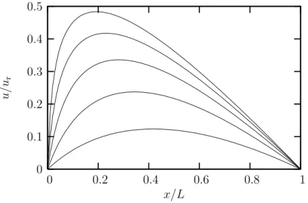
Figure 1. Solution profiles of the Rheinboldt’s example.
Analytical solutions can be easily integrated for these problems, and the results are
u(x)
ur
= 1
λa2 ln h
(exp(λa)−1)x
L + 1
i − 1
a x
L, (47)
u(x)
ur = 1
b ln
h
1 + (exp(λb)−1)x
L
i
. (48)
For growing value of the loading parameterλsolutions (47) and (48) exhibit sharp bound-ary leyers nearx= 0.
The first example is due to Rheinboldt [27] and the solution is shown in Fig. 1 for values λ = 1,2, . . . ,5. Since the flux in this example depends only on the gradient of u, the consistent Jacobian matrix is symmetric. Therefore, from the quasi-Newton family only the symmetric rank-two BFGS update formula is tested.
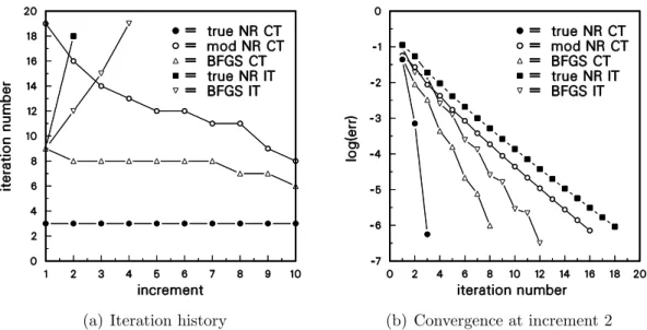
Convergence plots are shown in Fig. 2. In the computations the value of a = 1 and the increment size ∆λ = 0.5 have been used. It can be seen from the figures, that omission of the gradient dependent term Kg from the stiffness matrix causes severe
convergence problems, which cannot be overcome by using the BFGS update scheme. It is also worth noticing that the convergence rate of the Newton’s method with inconsistent Jacobian downgrades from quadratic to linear, i.e. as in the case of the simplified Newton-Raphson scheme. Convergence behaviour of the Newton’s iteration is unaffected from the discretizations used.
The example case with the exponential diffusivity is demanding. Both uniform and ge-ometrically graded meshes with 10, 30 and 100 linear elements, or 5, 15 and 50 quadratic elements or 3, 10 and 33 cubic elements have been used in the computations. The maxi-mum step-size which can be used in this example is ∆u0 =ur which can be used with the true Newton’s method with consistent Jacobian matrix.4 As in the previous example the Broyden’s quasi-Newton strategy is not successfull if the inconsistent Jacobian matrix is used. In figure 4 convergence behaviour is shown for four different strategies: true New-ton and the Shamanski’s higher order NewNew-ton with variable m (limited to m ≤ 3) and
4
(a) Iteration history (b) Convergence at increment 2
Figure 2. Rheinboldt’s example: convergence plots, CT=consistent Jacobian (tangent) matrix, IT=inconsistent Jacobian matrix (Kg omitted).
started after the first corrector iteration, thus abbreviated as NR-3,1. Methods are tested with both consistent and inconsistent Jacobian matrix. It is observed that the MR-3,1-method is converging rapidly and it is more efficient than the full Newton’s MR-3,1-method when consistent Jacobian is used. Surprisingly it is also rather fastly converging if inconsistent tangent is used i.e. whenKu is missing.
The iteration procedure using the additive decomposition described in equation (39) is not successful. Similarly to the diffusion-convection equation, based on the unsymmetric part of the Jacobian matrix (19), a characteristic non-dimensional elementwise P´eclet number has the expression
Peh = ∂D
∂u|∇u|h
(e)
D , (49)
where h(e) is a characteristic length of an element. For the constitutive model (44), the result is
Peh =b
|∆u(e)|
ur
, (50)
where ∆u(e)is the maximum nodal difference inufor an element. Therefore the condition (40) is not satisfied in the boundary layer of (48).
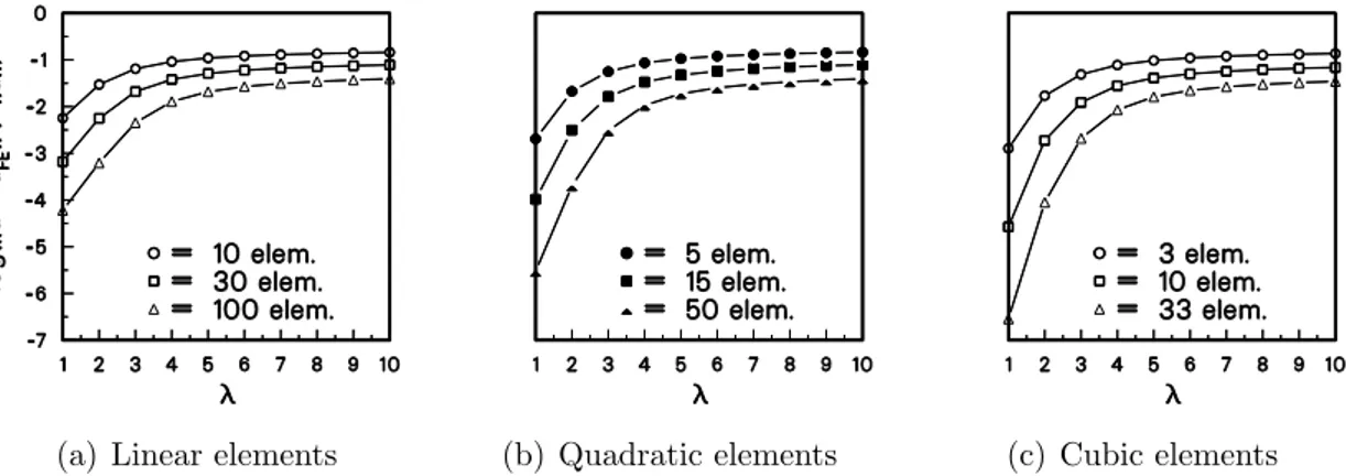
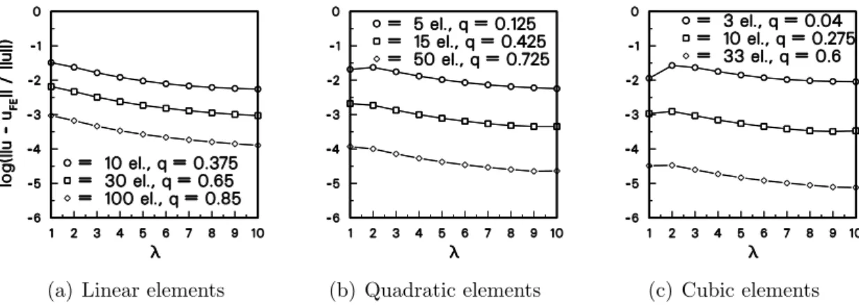
There is influence of the discretization to the convergence behaviour of the finite element solution. A boundary layer has a pollution effect which is clearly seen in Figs. 5 and 6. If a geometrically graded mesh is used the discretization error is more uniform with respect to the loading parameter λ.
The example with the constitutive model (44) is also computed in 2-dimensional do-main Ω = (0, L)×(0, L). At boundaries x =L and y =L temperature is prescribed by linear variation from zero toλur at (L, L). Analytical solution can be obtained by using a transformationu= (ur/b) ln(1 +v), giving a linear Poisson problem forv. Boundary con-ditions for this transformed problem are the following: v(x, L) = exp(λx/L)−1, v(L, y) = exp(λy/L)−1, v(x,0) =v(0, y) = 0. Solution for v is then
v = ∞ X
i=1
cnsinhnπx
L sin nπy
L + sinh nπy
L sin nπx
L
x/L
u
/u
r
1 0.8
0.6 0.4
0.2 0
10 9 8 7 6 5 4 3 2 1 0
Figure 3. Solution profiles for the example with exponential diffusion coefficient.
(a) Iteration history (b) Convergence at increment 3
Figure 4. Iteration history and convergence at increment 3 of the 1-D model problem with exponential diffusion coefficient.
(a) Linear elements (b) Quadratic elements (c) Cubic elements
(a) Linear elements (b) Quadratic elements (c) Cubic elements
Figure 6. RelativeL2-norm error of temperatureuof the 1-D model problem with exponential diffusion coefficient, geometrically graded meshes.
Figure 7. Randomly distorted 30×30-mesh and contour plot of the temperature field atλ= 10.
where
cn= 2
nπsinhnπ
1−(−1)nexpλb
1 + (λb/nπ)2 + (−1)
n−1
. (52)
Behaviour of this 2-D problem is similar to the 1-D counterpart. For growingλ bound-ary layers emerge for all boundaries. Convergence of the Newton’s iteration with consis-tent Jacobian is obtained in eight corrector iterations as for every step - stepsize ∆λ = 1 - as in the 1-D case. Mesh distortion do not affect the convergence when consistent Jaco-bian is used, however, the discretization error is larger with distorted meshes. Distorted mesh and the contour plot of temperature are shown in Fig. 7.
Transient examples
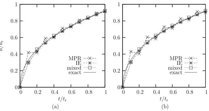
To demonstrate the effect of using a two-stage algorithm in order to damp the oscillations in the Crank-Nicolson scheme the following time dependent problems have been solved. The first one is a simple bar with temperature dependent isotropic material properties [23]. Both the thermal conductivity and the heat capacity are assumed to vary according to 1 + 12(u/ur) (u in ◦
C). All other surfaces except the surface x= 0 are insulated. The initial temperature is u = 0◦
C. The loading is a unit heat input through the surface
exact mixedIE MPR
t/tr
u
/u
r
1 0.8 0.6
0.4 0.2
0 1
0.8
0.6
0.4
0.2
0
exact mixedIE MPR
t/tr
1 0.8 0.6
0.4 0.2
0 1
0.8
0.6
0.4
0.2
0
(a) (b)
Figure 8. Temperature at the left end of the bar. (a) Numerical solution with bilinear elements and (b) with reduced biquadratic elements. Solid line indicates the exact analytical solution.
∆t = 0.1 s has been used, reference time is tr = 1 s. Using the one step implicit Euler method before switching to the midpoint rule inhibits the oscillations completely. It is also seen that oscillations of the midpoint rule computations are more pronounced for quadratic than for linear elements.
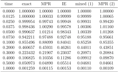
Cooling of a cube initially at constant unit temperature T0 = 1◦C and subjected to zero surface temperature when t > 0 is considered next. The analytical solution of this problem is given in Ref. [4] and finite element solutions e.g. in Ref. [30]. However, in their FE-analyses different initial conditions are used, in which the initial temperature varies from zero to one inside the outmost element layer. One octant has been discretized by 64 trilinear 8-node brick elements. Results are shown in Table 1. The time step has been ∆t = 0.0125 s. Clearly, the use of the one step backward Euler method prior the midpoit rule does not inhibit oscillations completely as in the previous example.
Concluding remarks
Table 1. Temperature at the center of the cube, 64 trilinear elements.
time exact MPR IE mixed (1) MPR (2)
0.0000 1.000000 1.00000 1.00000 1.00000 1.00000 0.0125 1.000000 1.00033 0.99999 0.99999 1.00065 0.0250 0.999954 0.99743 0.99948 0.99931 0.99420 0.0375 0.998436 1.00290 0.99578 1.00306 1.01160 0.0500 0.990637 1.01214 0.98343 1.00339 1.01268 0.0750 0.942211 0.97488 0.92748 0.95188 0.95661 0.1000 0.855496 0.88099 0.84041 0.85258 0.85355 0.2000 0.460657 0.45931 0.46261 0.44011 0.43851 0.3000 0.223432 0.21907 0.23037 0.20971 0.20884 0.4000 0.106825 0.10356 0.11286 0.09912 0.09870 0.5000 0.050973 0.04890 0.05514 0.04681 0.04661 1.0000 0.001259 0.00115 0.00153 0.00110 0.00109 (1) = First step with the implicit Euler method (IE) and the following steps with the midpoint rule (MPR).
(2) = with different initial conditions, identical to the results of Ref. [30].
Kiitokset
Jouni Freundille ja Eero-Matti Saloselle kommenteista. References
[1] L. Bernsp˚ang. Iterative and adaptive solution techniques in computational plastic-ity, Chalmers Univ. of Tech., Department of Structural Mechanics, Publication 91:8 (1991).
[2] K.W. Brodlie, A.R. Gourlay, and J. Greenstadt. Rank-one and rank-two corrections to positive definite matrices expressed in product form. J. Inst. Maths. Applics, 11 (1973), 73–82.
[3] C.G. Broyden. A class of methods of solving nonlinear simultaneous equations.
Mathematics of Computation, 19 (1965) 577–592.
[4] H.S. Carslaw and J.C. Jaeger. Conduction of heat in solids. Oxford University Press, 1962
[5] J.E.Dennisand J.J. Mor´e. Quasi-Newton methods, motivation and theory. SIAM Review, 19 (1977) 46-89.
[6] J. Freund and E.-M. Salonen. Heikkojen muotojen johtamisesta. Rakenteiden Mekaniikka, 23 (3) 1990, 18–61.
[8] Z.-J. Fu, Q.-H. Qin, and W. Chen. Hybrid-Trefftz finite element method for hear conduction in non-linear functionally graded materials. Engineering Computations. 28 (5) 2011, 578–599.
[9] M. Geradin, S. Idelsohn and M. Hogge. Computational strategies for the so-lution of large non-linear problems via quasi-Newton methods. Comput. Struct., 13 (1981) 73-81
[10] M.Geradin, M.Hoggeand S.Idelsohn. Implicit finite element methods. Chapter
7 in Computational Methods for Transient Analysis. Eds. T. Belytchko and T.J.R.
Hughes, North-Holland (1983).
[11] A.R. Gourlay. A note on trapezoidal methods for the solution of initial value problems. Math. Comp. 24 (1970) 629-633.
[12] T.J.R. Hughes. Unconditionally stable algorithms for non-linear heat conduction.
Comp. Meth. Appl. Mech. Engng, 10 (1977) 135-139.
[13] B. Irons and A. Elsawaf, Proc. U.S.-German Symp. on Formulation and Algo-rithms in Finite Element Analysis, Eds. K.J. Bathe et al., MIT, pp. 656-672 (1977) [14] C.T. Kelley. Iterative Methods for Linear and Nonlinear Equations. SIAM,
Fron-tiers in Applied Mathematics, vol. 16, 1995
[15] R. Kouhia. Newtonin iteraatiot ep¨alineaarisessa rakenneanalyysiss¨a. Rakenteiden Mekaniikka. 19 (4) 1986, 15–51.
[16] R. Kouhia and M. Mikkola. Some aspects on efficient path-following. Comp. Struct., 72, 1999, 509–524.
[17] R.W. Lewis, K. Morgan, H.R. Thomas, K. Seetharamu. The Finite Element
Method in Heat Transfer Analysis. Wiley, 1996.
[18] Q.H. Li and J. Wang. Weak Galerkin finite element methods for parabolic equa-tions. Numerical Methods for Partial Differential Equations. 29 (2013) 6, 2004–2024. [19] M. Luskinand R. Rannacher. On the smoothing property of the Crank-Nicolson
scheme. Applicable Analysis. 14 (1982/83) 2, 117-135.
[20] H. Matthies and G. Strang. The solution of nonlinear finite element equations.
Int. J. Numer. Meth. Engng, 14 (1979) 1613-1626
[21] G.Meurant.Computer solution of large linear systems. North-Holland, 1999. [22] M.Papadrakakisand C.J.Gantes. Preconditioned conjugate- and secant-Newton
methods for non-linear problems. Int. J. Numer. Meth. Engng, 28 (1989) 1299-1316 [23] S.Orivuori. Efficient methods for solution of non-linear heat conduction problems.
Int. J. Numer. Meth. Engng, 14 (1979) 1461-1476
[24] J. Ortega and W.C. Rheinboldt. Iterative Solution of Nonlinear Equations in
[25] R. Rannacher. Finite element solution of diffusion problems with irregular data.
Numerische Mathematik. 43 (1984) 2, 309–327.
[26] J.N. Reddy, D.K. Gartling. The Finite Element Method in Heat Transfer and
Fluid Dynamics. CRC-press, Computational Mechanics and Applied Analysis series,
3th edition, 2010.
[27] W.C.Rheinboldt. Numerical Analysis of Parametrized Nonlinear Equations. John Wiley, New York, 1986.
[28] Y. Saad. Iterative methods for sparse linear systems. PWS Publishing Company, 1996.
[29] H.A. van der Vorst.Iterative Krylov methods for large linear systems. Cambridge University Press, 2003.
[30] O.C. Zienkiewicz and C.J. Parekh. Transient field problems: Two-dimensional and three-dimensional analysis by isoparametric elements. Int. J. Numer. Meth.
Engng, 1 (1970) 61-71
Reijo Kouhia
Tampere University of Technology Department of Engineering Design P.O. Box 589, FI-33101 Tampere Finland