Implications of Ernbodied Technological Change for
Developrnent Economics
Sarnuel de Abreu Pessoa*and Rafael Rob'
Version 12 - Working Paper
May
2,2001
Abstract
Employing a embodied technologic change model in which the time decision of scrap-ping old vintages of capital and adopt newer one is endogenous we show that the elasticity of substitutions among capital and labor plays a key role in determining the optimum life span of capital. In particular, for the CD case the life span of capital does not depend on the relative price of it. The estimation of the model's long-run invest-ment function shows, for a Panel data set consisting of 125 economies for 25 years, that the price elasticity of investment is lower than one; we rejected the CD specification. Our calibration for the US suggests 0.4 for the technical elasticity of substitution. In order to get a theoretical consistent concept of aggregate capital we derive the relative price profile for a shadow second-hand market for capital. The shape of the model's theoretical price curve reproduces the empírical estimation of it. \lVe plug the calibrate version of the long-run solution of the model to a cross-section of economies data set to get the implied TFP, that is, the part of the productivity which is not explained by the model. We show that the mo dei represent a good improvement, comparing to the standard neoc!assical growth model with CD production function and disembodied technical change, in accounting the world diversity in productivity. In addition the
*Graduate 8choo1 of Economics, Fundação Getulio Vargas - Rio de Janeiro, Brazil. Current1y visiting The University of Pennsy1vania, [email protected], [email protected].
model describes the fact that a very poor economy can experience fast growth based on capital accumulation until the point of becoming a middle income economy; from this point on it has to rely on TFP increase in order to keep growing.
Jel Classification: D24, D33, E25, 011, 047, 049
Key words: Vintage CapitaL Embodied Technical Change, TFP Diversity, Elasticity of Substitution
1 Introduction
In 1960 Solow published a paper in which technologic change was embodied in new vin-tages of capital good. He showed that if the production function of a firm of any vintage is Cobb-Douglas (CD) and if the labor servicc direct to old vintages can be adjusted smoothly and continuously as the vintage ages, and, consequently, its productivity decreases, the con-solidate version of the model resembles the standard model with disembodied technological change. This correspondence result has turn the attention of the profession way of the specific investment assumption. Recently, it has been acknowledge that investment spccific technological change1 can help to understand some key stylized facts of the long-run path
of the US economy.2 In this paper, we argue that the embodied version of the investment
specific technological change with scrapping of old capital can describe some stylized facts for a cross section of economies. In particular it can help in understanding why poorer economy
presents a lower total fador productivity (TFP).3,4
In 1962 Arrow published his famous paper on learning-by-doing. Although the main issue of that paper was learning-by-doing and, hence, endogenous technical change, it does have
lInvestment specific technological change occurs when the innovation is attached to the acquisition of new units of capital. It could be because the new capital good embodied new technology or because the technology of producing new capital goods improves continuously.
2 Greenwood and Jovanovic (1999) provide a survey of the new literature on growth models with vintage capital.
3Hall and Jones (1999) OI Cavalcanti, Issler, and Pessoa (2000), among others, have documented this phenomenon.
~Prescott (1998) noticed the necessity of a theOIY that explain this regularity: lower TFP among poorer economies. Some suggested explanations are: Parent and Prescott (2000) argued that lower TFP is prevalent among poOIer economies due to monopoly groups ar unions which impede the adoption of newer technology; Parente, Rogerson, and \íVright (2000) maintained that the lackness of home production statistics could do a good job in explaining it, once we acknowledged that home production is much higher in poor economies.
a contribution to capital theory. In his model there is a Leonticf aggregator linking labor requirement and capital stock of a specific vintage. Due to the opportunity cost of employing an old vintage capital unit, which is given by the market wage rate, old capital is scrapped from production before became unproductive from a physical point of view. There is room for a theory that take into consideration economic depreciation as a different phenomenon than physical depreciation. vVhen we apply this idea to development economic the following result emerge. Poor economies are low wage economies; the opportunity cost of employing an old vintage capital in Arrow framework is lower. As a consequence, machines in average are older, which means that productivity is lower. Jovanovic and Rob (1997) worked in a set up which is a merge of Solow (1960) and Arrow (1962). From Solow they took the idea of embodiment in a context of exogenous technological change; from Arrow they took the idea of embodiment with a fix technology linking labor and capital, and, hence, scrapping. Parente (2000) and Mateos-Planas (2001) extend the Jovanovic and Rob model to take into consideration learning-by-using and human capital. As in Arrow's, these three papers employ a vintage capital model in which the finns combine capital and labor in a Leontief production function. Consequently, in order to focus on the quality trade off, the impact of distortion on the average quality of capital, they abstract totally the quantitative margin. In the usual neoclassical model an increase in thc distortion to capital accumulation produces the result that the higher the distortion, the lower the number of machines a plant employs, and, consequently, the lower the long-run income is. In these vintage capital models, due to the Leontief assumption, the quantity of capital that a firm employs is not sensitive to the leveI of the distortion. The effect is totally on the quality margin: the higher the distortion the longer it takes for the firm to update its capital stock, and, consequently, the lower the economy's productivity is. The economy is poorer because, in average, it employs older, that is to say, worse, capital.
quantity of capital of the newer vintage the firm has acquired.5 The First contribution of
the paper is to show that the impact of a distortion to capital accumulation on the optimum life span of capital depends critically on the technical elasticity of substitution among capital and labor. For the CD case there is no effect of capital price on the life span of machines. The intuition of this result is as follows: the opportunity cost of running an old vintage firm is the pay-roll. For the CD specification the wage payment by unit of capital does not depend on the cost of capital.
vVhen both margin are present, that is for the CES production function when the elas-ticity of substitution is lower than one and larger than zero, there are three effects of the distortion on long-run income. First, as in the usual neoclassical model, an increase in the distortion decreases the quantity of capital that each firms employs. This is the 'capital deepening' effect. Second, as in Arrow's framework, an increase in the distortion increases the life span of machines. This is the 'window' effect. Third, there is a effect which is the interaction of the increase in the life span of machines with the leveI of capitalization of the economy. v\Then the distortion increases, if the elasticity of substitution among capital and labor is lower that one, the life span of machines increases. This increase in the machines' life span make optimum for the firm to employ a higher number of machines, counteracting the first effect. Notwithstanding, we show that this effect does not supplant the first one.
The idea of the model is that a firm is a productive unit which employs one unit of labor service. The manager has to decide how many unites of capital she buys and how long she will employ them. \;\,Then the capital is old enough, she throws way the old capital and acquires newer unites. Because there are two margins of adjustment following an alteration on the relative price of capital, the quantity and the life span of capital, the long-run demand for capital is more elastic than the technical elasticity of substitution among capital and labor. 6
The Second contribution of the paper is to estimate the long-run price elasticity of the demand of capital in order to calibrate the technical elasticity of substitution among capital and labor. Employing Summers and Heston data set, we built a panel data with data for investment and relative price of capital. We consider a fix effect, which is associated with the TFP of the economy. Our result supports the view that the price elasticity of capital demand is lower than one, what means that the technical elasticity of substitution is lower
OIf this aggregator is Leontief we get Jovanovic and Rob model as a particular case. G\Vhen there is only the quantity margin both are the same.
than one; we reject the CD specification.
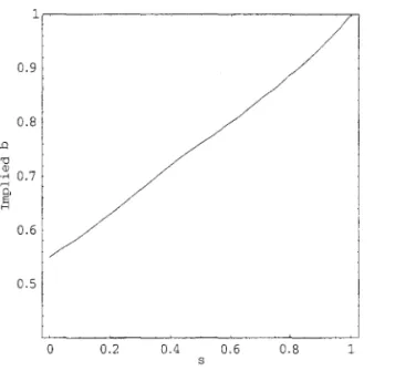
In order to calibrate the mo deI it is required to have a theoretical measure of aggregate capital. In the model of this paper there is no such thing as an aggregate production function. Firms from different vintage are evaluated differently. The Third contribution of the paper is to derive the price profile for a shadow second hand market for capital. The shape of the profile reproduces quite well empirical estimation of economic depreciation curve. In addition, the price pro file allows us to define precisely a concept of aggregate capital measured at market prices, which is in accordance with NIPA practicc. As a side result, we derive the fact, which agrees with the empirical evidence, that in poorer economies the price profile for used machines is less steep than in the developed economies.
It is worth to write some words about the hypothesis backing our calibration procedure. 'vVe chose the rate of technological change in order to match the long-run growth rate for the US output per worker. Implicitly, we are assuming that 100% of the technical change is embodied. We do not dispute that there is disembodied technical change. Our calibration procedure assumes that there is a perfectly complentarity among embodied and disembodied technical change.'
In our model therc are two concepts of the elasticity of substitution: one is the technical elasticity of substitution and the second is the price-elasticity of the long-run demand for investment. If there is no qualitative margin both are the same. In our framework they differs. Due to the possibility of saving capital employing longe r an old machine, the technical elasticity is lower than the price elasticity of the long-run demand for investment. The calibrated model for the US produces thc result that a plant-Leontief economy correspond to a price elasticity of 0.5; the time dimension adds a lot of flexibility.
After the calibration of the model to reproduces the US economy we rnake some leveI exercise. The Fourth contribution of the paper is to show that for very poor econornies, that is, economies whose relative price of capital is higher than two and a half times the price in the US there are sizable effects of capital's rnarket distortion on per capita incorne. For a price range between the price in the US and 2.5 times it the model predicts incorne leveIs difference that equals with the standard neoclassical model with disembodied technological change and CD production function. As a side result, the model provides a framework in
which a very poor economy, after some institutional reform that increases the rentability of the investment, undergo high growth fulled by factor accumulation without expressive gains of TFP; and that this growth los e momentum when the economy became a middle income one. It is possible that a computable version of the paper's model which investigate the transitory dynamic of a poor economy in succession of a reduction in the relative price of capital produces path that reproduces the East Asian recent economic growth experience, as documented by Young (1995).
The capability of the mo deI in producing high leveI effects is an artifact of the CES specifications with a less than one elasticity of substitution. For this case the Inada condition at the origin for the Marginal Productivity of capital fails. Hence, the neoclassical model of capital accumulation with a CES Production Function and disembodied technological change generates leveI effects which equals the mo deI developed in this paper. The difference is that our specification produces very distinct result for the economic depreciation and for the capital-output ratio. For our specification, given that the depreciation is an economic phenomenon, it reduces a lot for very distorted economies, due to the increase in the life span of capital, and, consequently, the capital-output ratio does not decreases as much as it would for the standard neoclassical model. In particular, for the calibrated value of the technical elasticity of substitution, 0.4, the capital-output ratio, when the used capital evaluated in units of new capital is measured at domestic prices but the new capital is measured at international prices, presents an almost constant behavior.
In the last part of the paper, employing the consolidate version of the model, we make a development decomposition exercise: we plug in the equations that describe the long-run equilibrium of the economy the observation on education attainment, long-run investment, and relative income for a cross-section of economies and we get the implied TFP, that is, the part of the diversity in productivity that is not explained by the model. The Fifth contribution of the paper is to show that this residue decreases a lot after taken into con-sideration capital's quality. Our conclusion is that capital quality is an important ingredient for understanding income inequality among economies.8
This paper has the following organization. The problem of the firm, it existence,
unique-60ur result are in front disagreement with Parente's (2000). In his paper there is not a market evaluation of capital from different vintage, and, consequently, he does not have a good theoretical concept of aggregate capital in order to match the NIPA data of it. That is the reason that makes his calibration so different than ours.
ness, and comparative statics is study fully in the following and the ensuing Sections. The fourth Section derives the price profile for a second-hand market for capital and investigates the functional distribution of income for a firmo The next Section derives the macroeco-nomic aggregates and the sixth Section characterizes the Planner Economy. In the seventh
Section the model is calibrate to reproduces some features of the US economy in order to asses, in the eighth Section, the capability of the model to describe relative income diversity given capital price differences among economies. The calibration of the technical elasticity of substitution is performed in the ninth Section and the subsequent Section presents the development decomposition exercises. The eleventh Section concludes.
2 The Firm
The economy is inhabited by a continuum of individuaIs with measure 1. Each individual is the owner of an equal share of the economy outside wealth, the total value of the firms, and supplies inelasticly one unite of labor effort. The firm is an infinitum horizon entity which is characterized by an unity of entrepreneur capability and an initial planto The entrepreneur can supervise one labor. A plant is described by the vintage that its capital stock belongs with, s, the technologicallevel associated with this vintage, A( s), and the quantity of capital that it employs, K (s). \Ve assume that the frontier technological leveI evolves exogenously as A(t)
=
A(O)e9t, although the technicallevel of the vintage-s plant is fixed. Let Y(s, t) be the production in time t of a vintage-s planto We assumeY(s, t)
=
e-c5(t-s) max {O, Y(s)} (1)\vhere
Y(s)
=
B[(1-
a)(eq,(h)A(s))";;l+
aK(s)";;l] "=-1, (2)O
<
a<
1 is the distribution parameter of the CES production function, and (J is the elasticity of substitution among capital and labor. Although we are interested on the case O :S (J :S 1 the results apply for an open set including (J=
1, the Cobb-Douglas case.factor intensity, the firm faces a CES production function, given by (2). After installing a plant it is not possible to freely adjust the number of workers to the changing in the environ-ment. That is, after deciding that one worker is going to operate K(s) units of capital, the entrepreneur cannot change this ratio. Labor, as capital, became a fix cost. Obviously, when the moment of renovation has arrived the firm, again, faces the possibility set of technology represented by (2).
This quite unusual production function is required in order to get an easy dose form analytical solution. In our set up capital, and the technological leveI attached to it, is a fix factor. The firm once and a while adjusts it to the optimum leveI, but between two consecutive changes in technology it is not possible to adjust the capital stock. If we would have considered that labor is a fiexible factor the relative marginal rate of substitution among capital and labor would be continuously changing, making the model not as analytically savable for the CES specification as the mo deI that we consider in this paper.
There are tl,vo others possible environment which, as far economics is concerned, are equivalent to the environment in this paper. First, it is possible to consider that the economy is a owner-Iabor economy, that is, each firm is run by the worker which is also the owner. In this context we consider imputed wage rate instead of the market wage rate for the production factor labor. Second, it is possible to assume that a firm and a plant are the same entity. \Vhenever an old plant is scrapped from production the entrepreneurial capability attached to it disappeared. Under this interpretation there is a perfectly elastic supply of entrepreneurial capability in the economy, such that in equilibrium there are firms closing down and others opening up. Both interpretations are possible, and from the point of view of economics they are equivalent. This last formulation resembles Arrow's and Solow's; the labor-owner formulation was employed by Jovanovic and Rob. In the interpretation in this papel', the entrepreneur is the decision maker. It supervises the worker, pays the salary, distributes the firm's cash fiow net of wages to the share-holders, and issue new equities in order to buy a new plant when renovation time has arrived. For the rest of this paper a vintage-s firm is a firm currently operating a vintage-s planto
Three comments are worth doing at this point. First, it is considered a CES production function because, as we will see, the elasticity of substitution among capital and labor plays a very important role on the impact of the distortion on the life span of machines, and con-sequently, on the average age of machines in the economy. Second, although, as necessarily is the case in vintage capital models, the technological change is embodied in the capital,
it affects labor's productivity. Consequently, when the firm updates its capital stock the labor productivity, A( s), increases. It is known that in order to get a balanced growth path in a capital accumulation model when the production function is not Cobb-Douglas it is necessary to assume that the technologic change is labor-saving. The formulation (2) shows that it is possible to consider an embodied technical change growth model whose technical change is labor saving. In other words, there is no conflict among the embodied hypothesis and the nature of the technological change. In addition we think that this is the better way of considering embodied technological change. By technological change associated to capital we mean an increase in capital's quality as time goes by. If the variable A( s) that represents this qualitative change were multiplying the capital, instead of the labor, this technical change would be observational identical to an increase in the productivity in the capital industry, that is, to a continuously reduction in the number of forgone consumption good that is required in order to get one unit of capital. In our model a better machine is a unite of machine that makes the worker a better work. Third, the total factor productivity of a vintage-s plant depreciates at a rate b. Although the number of machines is not affccted by physical depreciation, it does have a negative impact on the productivity, and this impact does not change the marginal rate of substitution among capital and labor. As we discussed last paragraph, this formulation is convenient from the analytical point of view. In addition, we think that this formulation is theorctically consistent with the labor-saving technologi-cal change assumption. Given that a better machine increases the labor productivity it is reasonable to assume that when the machine ages depreciation affects both, the physical dimension of and the productivity factor attached to it.
Given that we intent to employ this model to make some cross country exercises we consider that different economies differs in three dimensions. First, although the vintage capital model helps us to understand diversity in TFP, we allow for others source of difference in productivity. Ü The height of the production function, B 1 describes the portion of the diversity in TFP which is not accounted for capital's quality and quantity. Second, although this paper is not on education decision, we know that diversity in educational endowment has a important impact on the capitalization leveI of the economy and labor productivity. Consequently, we take into consideration the impact of the educational leveI of the active population, h, on labor productivity. We assume a Mincerian formulation as ecjJ(h) , where
the function rfJ( h) relates increases in the average number of year of education of the active population with the increase in wages.10 Finally, the third source of cross country diversity is on policies that alter the relative price of capital.
The sequence of the decisions made by the firm goes as follows. Let take as an example a firm currently employing a vintage-s planto Being a vintage-s plant means that some time ago, specifically, in time s the firm had chosen the quality of the new machine, which was the frontier one (the cost of new unit of capital does not depend on the quality of it); and the number of machines that it will operate during the next period of time (until the next changing in technology). Consequently, the choice of A(s) and K(s), the plant's choice, was done in s. Let' s call V (K ( s ), t) the vaI ue function in t of a firm w hich operates a plant with
K units of vintage-s capital (which implies that the labor productivity associated with this capital is A( s)). The maximization problem of the firm is
V(K(s), t)
=
{l
T+S
,ma~ < e-r(t'-t) (Y(s, ti) - w(t' )) dt'
I,K(T,,,) t (3)
+e-r(T+s-t) [1I(K(T
+
s), T+
s) - pK(T+
s)J} .where w(t) is the market wage rate, p is the relative price of machines, and r is the interest rate (which is constant for a balanced growth path). At time T
+
s the firm throws way the old plant and acquire a newer and better one. Consequently, in addition to physical depreciation there is technological depreciation.The FOC that solve the maximization problem (3) are
and
for T
8V(K(T + s), T
+ s)
for K(T + s): 8K(T + s)=
P0= Y(s, T
+
s) - w(T+
s) - r [V(K(T+
s), T+
s) - pK(t+
s)]8
+-
[V(K(T+
s), T+
s) - pK(T+
s)]. 8TlOIn our development decomposition exerci se we employ Hall and Jones (1999) data on e'P(h).
10
(4)
The envelop condition is
dV(K(s), t)
=
3V(K(s), t)=
j.T+S e-r(t'-t)3Y(s, t') dt'dK ( 8 ) 3 K ( s ) t 3 K ( s ) . (6)
From (4) and (6) it fo11ows that
j
T+S e-(r+6)(t-s)3Y(s) dt=
8 3K(s) p. (7)
Let ca11
h(r
+
5, T)==
j
T+S e-(r+6)(t-s)dt = - - - - -1 e-(r+6)TS r
+
5(8)
If the interest rate is constant (stationary state), the condition (7) can be rewritten as
.
(Y(S))~
aBh(r
+
6, T) BK(s)= p.
(9)Condition (9) is equivalent to the modified golden rule for capital accumulation in the standard Cass-Koopmans model. It fix the present value of the marginal productivity of capital to the relative price of it. In a balanced growth path the market interest rate is equal to the intertemporal discount rate plus the growth rate divided by the intertemporal elasticity of consumption. In order to understand the intuition behind the other first-order-condition, equation (5), let rewrite it as fo11ows
3
Y(s, T
+
s) - w(T+
s)+
3T [V(K(T+
8), T+
s) - pK(T+
s)]r [V(K(T
+
s), T+
8) - pK(t+
s)].It expresses that the benefit of postponing in one unit of time the upgrading time, which is the addition of the net-of-wages value-added in the old plant with the increase in the quality of the plant due to this postponing, should be equal to the cost of postponing, which is the opportunity cost of not using now a newer vintage capital.
From (2) we know that
Y(8) _ [ _
(e1'(h
JA(S))
a;;11
a~1
From (9) and (10) it follows that
where
k*
=
K(s)- eq,(h) A( s) [
Do"-l _
a]
1-'-'-0-l-a
D=~
P
- ex Bh(r
+
D, T)·(ll)
(12)
.:iote that k* is per worker capital measured in efficient units, not controlled for depreciation. Let's indicate by
f*
the per firm (which is equal to per capita) output measured in efficient units. It follows from (10) that*_ Y(s) [ * ~]0-~1
f
=
BA(s )eq,(h)=
1 - a+
a (k ) o- • (13)Evidently, (ll) only makes sense if DO"-l - ex
>
O, which implies that(14)
should be verified for a valid equilibrium.
3
Optimum Time Between Switches
3.1
FOC
The labor's productivity associated with the vintage s capital stock evolves according to
A(t)
=
egt, where 9 is the exogenous technological change. In the stationary state thecapital-labor productivity ratio is constant (it follows from (ll)) and the capital-output ratio is constant (it follows from (10)). We can rewrite condition (5) for the optimum switching time as
0= Y(s, T
+
s) - w(T+
s) - r [V(K(T+
s), T+
s) - pK(t+
s)]+ V(K(T
+
s), T+
s) 8 V(K(T+
s), T+
s) _ K(T+
s) 8K(T+
s). (15)V(K(T+s),T+s)8T . PK(T+s) 8T
For a balanced growth path
1 aK(T+5)
K (T
+
8) aT=
g,and
1
a
V(K(T + s), T
+ s) aT V(K(T +
s), T + 8)=
g.Consequently, after taking into account (2), (15) can be written as
e-OTy(s) - egT w(s) - (r -
g)
[V(K(T + s), T+ s) - pK(t + s)]
=
O. (16)Let ca1l1l the firm's cash fiow for t E (T
+
5, T+
T+
s].
We knowex
V(K(T + s), T
+
s) - pK(t + s)=
L
(e-(r-g)T)' 11i=O
11
1 - e-(r-g)T'
But,
11 h(r
+
6, T)Y(T + s) - h(r - 9, T)w(T + s) - pK(T + s)egT [h(r
+
6, T)Y(s) - h(r - 9, T)e gT w(s) - pK(s)](17)
egT { [h (r
+
6, T):(±
B h (r : 6, TJ (7 - 1] K ( s) - h (r - 9, T) w ( 5) }, (18)where the last equality follows from (9).
Substituting (18) and (17) into (16), it follows that
(19)
should be verified for the optimum time.
frontier produces scrapping, and, consequently, the continuum increase of the wage rate. 11,12
Consequently, the labor cost of the firm-unit is independent of its action. Note that wc can rewrite (19) as folIows
li TI - e-(r-g)T 1 - e-(r+Ó)T K (s)
-e-(g+ )
+
=
p - - .r-g r+6 Y(s)
lvIaking the transformation u
=
e-gT , a==
!. and b _ Q we get9 9
1 - ua+b 1 - ua - 1
--b-Y(s) = gpK(s)
+
ul+b Y(s).a+ a-I
This last equation is identical to equation (29) at pg. 163 in Arrow (1962) for the case
D
=
O. L3 The neoclassical model, vvith exogenous and embodied labor-saving technologic-change with scrapping is isomorphic to Arrow's learning-by-doing modep4 In addition, as we wilI see later, it has the folIowing interpretation: the present value of the value-added in a firm-unit between two consecutive switches, 1~~t Y (s), is equal to the capital cost of the firm-unit, gpK(s), plus the present value ofthe wage rate, Ul+bl:~al-ly(S).From (9) we know that Y(s)
=
C"Bh(~+Ii,T))
a BK(s). Consequently, we get0= e-ÓT (aBh(rP
+
D, T)) a B - 1_re~/;_9)TegT
[h(r+
6, T) (aBh(rP
+
6, T)) a B -p] .
(20) Equation (20) highlights the role played by the elasticity of substitution between capital and labor in assessing the impact of capital's price on the optimum time between two consec-utive switches, that is, on T. For the Cobb-Douglas case (cr
=
1) the machines' price cancels out in the expression. The window does not depend at alI on this price. When this price increases the window does not change and, it folIows from (11) and (12), that the adjustment is only on k*, the quantitative margin. Another interesting property of the model is that, due to the linearity among production flow and the number of machincs, which is expresses11 For an endogenous growth version of the model of this paper, scrapping is creative destruction. We deal with this issue in a companion paper.
12In the short-run a vintage is a non-reproducible factor. That is the reason of the rent. However, in the long-run the unique no-reproducible factor is labor. We have unbound increase of the imputed wage rate.
lJHe considered an One-Hoss-Shay process of physical depreciation. 14The optimality properties are different.
by (9), the model is separable: first we solve (20) for optimum T, given the parameters (p, r,
B, D, and g), and then, afterwards, we substitute the optimum Tinto (9) to get the optimum capital-output ratio. Finally, it follows from (12) and (20) that the choice of both margins depends on the ratio
13'
3.2
Uniqueness
Condition (20) can be rewritten as
1 - e-(r-g)T 1 - e-(rH)T p (1 _ e-(r+Ó)T) cr
H(T,p) _ e-(gH)T - +oF(_)l-cr
=
O.r-g r+D B r+D
In order to make the domain compact let make the following change on the variable
what implies that
Substituting this last equations into (21), it follows that
.\di 1 - u~ 1 - u_r~_6 cr( p )l-cr (1 _ u_r~é) cr _
H(u,p) _ u 9 - - - -
+
a - - O.r-g r+D B r+D
The graph of the function H displayed in Figure 1 motivates the prove of uniqueness. The function H (u) has the following features:
) {
OifO<(}<l
H(l
=
-13
if O"=
O.(21)
(22)
(23)
(24)
/ "
o~---~· --~\
-2
o
0.2 0.4 0.6 0.8 1u
Figure 1: Example of the FOC for optimum T for (J = 0.5
(
.':.±i)cr-l
1-u 9
r+D
The derivative of H presents the following characteristics:
and
oH
Ou (O)
=
0,oH
(1)= {
ou
°
if (J=
0,-00 if
°
<
(J<
1,-Q. if (J
=
1.9
16
(25)
Substituting (22) into (25) we get for an interior equilibrium that
2.
{g
+
6 1 - u7
r+
6 u7
[1 - ur!/5
E..:!:i 1 - u~
1 }
U9 - - - a - u 9
9 , - g 9 l-u~
,+6
r-gu% {9+61-U
7
_a1'+6 u7
[1-U~
-u~I-U7l}
r-g :::H. r+ó T-,9
9 9 -g- 9 l-u9
9
9ub {
1 -
ua-I ua-I[1 -
ua+b1 _
ua-I] }- (l+b) 1 -a(a+b)1 +b b _ul+b ,(27)
9 a - - u a a
+
a-Iwhere
r 6
a
== -
> 1 and b== -.
9 9
It is possible to rewrite (27) as follows:
oH
1 •
ou
uUbl-Ua-1 { 1 [(a-1)ua-1 (a+b)ua+b]}
(l+b)- l a
-9 a - I 1
+
b 1 - u a-I 1 - ua+bub 1 - ua-I { 1 [(a - 1)ua-1 (a
+
b)ua+b] }>
(l+b)- 1 - - --~~-9 a-I 1
+
b 1 - u a-1 1 - ua+b>
O
(28)if
(a- l)ua-1 (a+b)u a+b
1 _ ua-1 - ' 1 _ ua+b
:S
1+
b. (29)In order to establish (29) note that
This last result follows because -In ua
:S
I~~a, for O:S
ua:S
1. Consequently,or
B " p <
p
=-
- - ( } : , , - 1 .,+6
(30)If (30) is satisfied, we have established uniqueness for the balanced growth path solution for this economy under the proviso that it exists, which implies that (14)
is satisfied.
But, it is possible to rewrite (22) as
1-U
7 {
E..±.d-u~
,+6
s: u 9 r+6
, +
u , - 9 1 - u-g-which means that in equilibrium
r - q
E..±.d - u-g-
,+
6' 1 - u 9 ; : :-2±§.
, - g 1-u 9
< 1. (31)
If (30) is not satisfied the firm does not update the capital, and, consequently, there is no growth.
3.3 The Global Maximum
So far we do not know if the solution for the FOC is the global optimal of the firm's value function.15 As we will see, the value function is not concave in the variable T, hence, requiring
another approach to find the solution for the program of the firmo In this subsection we build the value function and show that the FOC (4) and (5) solve for the global maximum of the firm's value function. The prove is constructive. First we show that if p
< p
the firm updates its technology an unbound number of time. Second, due to the stationarity of the environment faced by the firm and to the recursive structure of its maximization problem,15In order to simpli(y the notation, in this Subsection edJ(h) = 1.
the choice made by the firm in efficient units does not change. \Vith this information it is possible to compute explicitly the value function. Given this value function we make its dominium compacto Then we show that (4) and (5) provide its global maximum. The first step is to note that it follows from (14) and (18) that the strategy described in the last subsection produces a strictly positive value for the present value of the value-added between two consecutive switches in the firmo Consequently, any candidate a optimum strategy has to provide a higher value for li.
\Ve can write the firm's value function as16
V(K(s), t)
= e-
6(t-s) h(r
+
D, T1+
s - t)Y(s)where the firm employs the vintage-s
+
L:l
~ capital for Tn+l units of time. :-Jote thate-r(t-S)V(K(s), t)
+
h(r+
D, t - s)Y(s)h(e
+
8, T,)Y(s)+
~ e-'L~,
T,[h(T
+
8,1~+1)Y
( K s+
t,
'li )
pK
(s
+
t,
1i)
1
V(K(s), s).Given that V(K(s), t) is an increasing linear transformation of V(K(s), s) we can, without lose in generality, to study the value function V (K (s), s) reminding the K (s) is a predeter-mined variable.
The next step is to show that if p
>
p
the firm at least change the technology once. Let assume that the firm never change the technology. Its value would beY(s) V(K(s), S)No Renovation
=
- - cr+u
vVe compare this value with the alternative value g'iven by the following action: at time TI
+s
to change the technology and from this time on to pursue the optimal strategy characterized in the previous subsections. The firm get
V(K(s), S).,'dtermuivc
=
where
because p
>
p.
But, for TI big enough it is true thatHence, it follows the resulto Employing a straightforward restatement of this argument we show that N, the number of switches, is unbound. Let consider a firm \vhich has switched
N times, and let calculate its value function under two strategies. First, never switch again; second, to switch in time s
+
~~il1i and then commutate to the optimum strategy. The value function for the first strategy can be written asV(K(s), S )1\0 Rellovation After N
= e-
6(t-sl h(r+
15, TI+
S )Y( s)The alternative would be
V(K(s), S)Altcrnative After N
=
e-6(t-slh(r+
15, TI+
s)Y(s)"B\lOTECA MARIO HENRI:lUE SIMOISEI
~!lNo.clo GETULIO VARGAS
20
, N , 1 - e- r+u TN+1
[
( ,)
( N)
(N)
+e-rls+L=l
Ti) T'+
b Y s+
~li -
pK s+
8
Ti1 ( b T)BOCY
(N+l)]
+e-rTN+1 l T'
+ "
-
p K s+ ""'
Ti1 - e-(r-g)T L...
i=l
(33)
where
Comparing (32) with (33) it follows the resulto
The next step is, benefiting from the recursivity structure of the firm's value function and from the stationarity of the environment in which the firm is embedded, to show that the switching time are equally spaced. Let s
+
T be one instant just before the first choice of a new capital unit, and let U(s+
T) ::::::
V(s+
T,
K(s)) - pK(s+
T)
be the net value function. Reminding that A(s)=
A(O)egs we can writeU(s+T) [
~
"-"l":':1
~
----=---
=
h(T'+
b, TdB 1-a+
ak(s+ T)-G
-
pk(s+
T)A(O)eg(s+T)
where17 k(s) :::::: ~f:].
_ V(s) Let define U (s)
=
A(O)e9S 'where
We have
o
<
e-(r-g)T1<
1,and the choice variables are k (s
+
T) and TI' 80 far I do not know if the FOC characterizes the optimum 18 TI, but given recursivity we know that in time s+
T
+
Tl the decision maker faces 17In this Section and iu the Section on the Planner solution k(s) = ~r:j.In the Section on aggregationthe same problem as it faced in time s+T. Consequently T2
=
TI and k(s+T+Tl )=
k(s+T).By finite induction it follows that for any integer i, Ti = TI and k(s+T
+
L~=l Ti) = k(s+T).It is possible to calculate explicit the value function U(s). We get
~
1
l~~:b
B[1 -
a+
ak(s+
T)O~l]
O~l
-
gpk(s+
T)U(s+T)=a_l l_vaI
a-I
where a, and b as defined in (27) and v
=
e-gT1. So far we have not said anything about the initial capital, k( s). vVe investigate the balanced growth path solution. Consequently, it is natural to assume that the initial condition for the capital stock is compatible with that
~ ~
solution, that means, let assume that k(s) = k(s
+
T). But if k(s) = k(s+
T) we know thatT
=
TI, which for simplicity we write19 T. Now we can compute the firm's value functionevaluated in efficient units. \Ve get
lV(s k(s))
==
V(s, K(s))=
e-(r-9)Tu(s+
T)+
pk(s), A(O)e9S
ua-1
l~:b-"-b
B[1 -
a+
akO~l] o~l
- gpk1 _
uo+b [0-1]
o~l
---'~---;-J - - - - " ' - - -
+
B 1 - a+
ak (s) - o (34)a-I ~ a+b
a-I
\vhere we know that, due to construction, k( s) is equal to the value of k that maximizes the transformed firm's value function, W(s, k(s)).
V/e know that
and
where
O:::;
u:::;
1,_1_B
[1 _
a
+
a7t~1]
o~l
-
pk
=
O
T+6
The chosen capital stock is lower than
k
because for k >k
the present value of thevalue-19S0 far we have already not proven that this T is equal to the optimum one derived in the first part of this Section.
0.6
Figure 2: Firm's Value Function under the standard calibration for the US (Section 6)
2.5 5 7.5 10 12.5 15 17.5
added, assuming that the firm never upgrades again, is negative.20 If O
<
p<
p
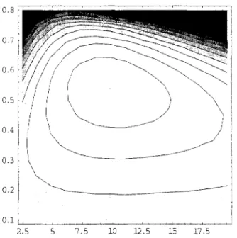
we alreadyknow that for k given by (11) and T given by (22) the value of the firm in efficient unitcs, W(s, k(s)), is positive and that the valuc added between two switches in present value is positive. Consequently (34) has and interior maximum. For a continuum function defined in a compact dominium, if the maximum is interior it is characterized by the FOC. If the solution for the FOC is uni que it correspond to the global maximum. Simple computation shows that (11) and (22) are the FOC for (34). Figure 2 presents the 3D graph and Figure 3 the contour plot for the firm's value function in efficient units for the model's calibration for the US economy (Section 6).
So far we have not yet chosen that the market value of a firms, the value given by (34) net of wages and net of the market cost of the initial capital, is zero. This condition
is required to characterized the equilibrium (otherwise an unbound number of firms will be open up). To accomplish this we need a price theory of used capital. This is done in the next Section.
3.4
Comparative Statics on T
From (22) and (27) it follows that
20Note that du
dp
for any O S T < 00.
oHI
ap
u*-
~~
lu*
1-0"
dT(~)I-(T
(I-r~;)
(T---~----~---~
t ~ r+o-g (
:::H)
(T-Ip+óU9 I-u 9 _ O"a(T(E.)I-(T~ I-u 9
P r-g B 9 r+ó
p
§ O whether O" § 1
24
because
oH I 9
+ [;
Q.1
-
u~
CT( P )l-CT Ur+:-g
(1 _
U~,';8
) CT-l- u*
=
- - U 9 - - - - CTa - > O.ou
9 T - 9 B 9 T+ [;
That is the main resulto The impact of machines' relative price on the optimal windO\v depends on the elasticity of substitution among capital and labor. In particular, if CT > 1
the effect is on the opposite direction: the higher the relative price the shorter the machines' life span! The intuition of the result is the following. An increase in capital's relative price induces a reduction in the quantity of machines employed in production. \iVhether the elasticity of substitution is high or low, capital and labor, in effective unites, are complements or substitutes. In the first case the reduction in the quantitative margin implies a reduction in labor's services, and in the former situation an increase in labor's services. The firm increases or reduces the life span of machines in order to employ less or more labor services respectively.
If the elasticity of substitution is one these two factor balances perfectly. Another way of thinking is the following. The elasticity of substitution determines if quality and quantity are complements or substitutes. If the elasticity is lower than one they are complements. and, consequently, an increase in the relative prices reduces both, the quantity and the quality of capital.
Another implication of the model is that the distributive factor of the CES production function alters the optimum life span of machines. Calculating
oH
=
CT-l(E.)l-CT 1 - 'u-9 O(
r+6 ) CT
oa
CTa B T+ [;
>,
which implies that
oH
du
= _
oa I u*<
OoH .
da ou
lu'
Cobb-Douglas case: although there is not anymore any impact or machines' price on the window, it is still true that the higher the capital's share or income the longer is the lire span or machines. Consequently, ror that plants whose share on income or machines is very large -metallurgy, ror example - the lire span or the plant is very long; ror that plants \vhose share on income or machines is low - ror example, researcher employing personal computer in a office - the lire span or the computer is low. Saying differently, even ir the technological change in metallurgy is as fast as the one in computers, the life span or a metallurgical plant is longer, only because it is capital intensive comparing with an office with computers.
It seems to me that this last result can be stated in a very general way. It is possible to imagine that the production or anything is an aggregation or many tasks. In order to perform a task, capital and labor, both specific to the particular task, is required. Than we can think that the CES aggregator
(36)
describes the production or one task. Consequently, the production or the product can be represented as a complicated aggregation or many different black-boxes-tasks like (36). For example, to produce cars it is required office work and plant work (white collar and blue coUar works). For each one or these two different tasks there are a specific CES aggregator. The automobile industry updates its machines in the plant, but also its personal computer into the office. Office-like task is labor intense, low Q, and, consequently, the time span
of personal computer is lower, even ir the exogenous technological change is not different among tasks.
4
Second-Hand Market for Plants
The basic economic productive unit in the economy is a vintage-s planto A vintage-s plant is a technology, A(s), plus a quantity or capital, K( s), which has been bought anew in time s. In this paper embodiment has two distinct features. First, in order to have a better technology the firm has to buy a new capital unit. Second, there is a perfectly complemantarity among capital of different vintages. Once a new machine is bought, the old one get useless. Consequently, the cost or using a old machine is not only the lower productivity capacity of it; it is also the labor opportunity cost or not using a better one.
This last feature, as we have seen, produces capital scrapping. Another implication of it is that the market prices of a vintage-s plant declines at higher rate than machines physical and technical depreciation, which is given by c(g+Ó)(t-s). As we will see next Section, the model delivers two measure for aggregate capital stock: in efficient units and at market prices. For an economy whose relative price of capital is low, which means that capital renovation and scrapping is high, these two way of account the capital stock will produce quite different estimates.
In this Section we derive the price profile for a shadow second-hand market for capital. It has the following organization. In the first Subsection we derive the price profile for used capital. In the second Subsection we study the rental price of capital implied for this price profile and derive the wage rate of the economy and the functional income distribution of the firm's value-added (that is, how the value-added in a firm is appropriated by the capital and the labor). In the third Subsection we show that the market value of a vintage-s plant, that is the present value of a vintage-s plant net of the market value of its capital and of wages, lS zero.
4.1
Price Profile
For the sake of comparison, let's study the price profile under Jorgenson (1974) framework.21
He assumes that the production function of a firm created in time s can be represented by
F (L(t),
li
e-(g+ó)(t-t') I(t')dt') , (37)where I(t') is the investment done by the firm in time tI. In that case e-(g+ó)(t-t') units of vintage-t' capital is a perfect substitute for one unit of new capital. Let q( t - s) be the price of a t - s age machine in (37) which is going to be scrapped after T periods of use. In present value, we get
q(t - s)
rT-(t-s) -(r+b)ud
e-(g+ó)(t-s) Jo e u
rT e-(r+b)udu Jo
e-(g+b)(t-s) h(r
+
6, T - (t - s))h(r
+
D, T) .vVhen there is no scrapping it follows
lim q(t - s)
=
e-(gH)(t-s).T-+oo
In addition, due to this perfect substitutability among different vintages assumed in the production function (37), there is no economic rationality to scrap any machine from pro-duction.
In order to derive the price profile of used capital, which in our framework is also the price profile for used plants, we imagine the existence of a shadow second-hand market, and ask for the price profile which supports a zero trade result in this market. That will be the equilibrium price profile for the economy and the market evaluations of an old plant. In
addition, under these price, the entrepreneur is willing to by a new machine after scrapping the old. Let call w(t) the cash fiow by unit of time of the following action of an agent: to buy a vintage-s firm22 in time t, run it till time t
+
!::lt, and then resell it.23 We havew(t)!::lt
i
H 6 t
--'!..-e-ó(t-s) K(s) t e-(rH)(t'-t) B
[(1 -
a)(k*)-";;-l+
a] ,,-I dt' - p(s, t)K(s)+e-r6tp(s, t
+
!::lt)K(s) ,where p( s, t) is the market price in t of a unit of capital of a vintage-s firmo Due to the optimum solution in the primary market, we know that
K(s)
=
e-g(t-s) K(t),and, consequently, we get
j
t+6t _,,_e-ó(t-s) t e-(rH)(t
l
-t)B[(l_a)(k*)-o-;;-l +a]"-l dt'_p(s,t)
+e-T6tp(s, t
+
!::lt).Due to non-arbitrage condition, ;i~~!::lt should not be a function on s.
22 A vintage-s firm is a firm which currently is running a vintage-s planto In order to run the vintage-s capital the economic agent has to have one unit of entrepreneurial capability. That is the reason that in the thought experiment considered in the text the agent buys a vintage-s firm and not a vintage-s planto
23Later, we will show that this cash-fimv is exactly the wage rate.
Taken a Taylor decomposition up to first-order terms we get
where C
==
~~~~. After discarding second-order terms and guessing that the profile depends on the age of the firm, we are left with(38)
whose solution is
{ [
"-1]
,,~1 e-(r+6)T e-(r-g)T } p(T)=
erT B (1 - o:)(k*)--"+
o: - C+
D ,r+D r-g
where D is an integration constant. We have an initial condition, p(O)
=
p, and terminal condition, p(T)=
O, in order to determine C and D.In order to understand the economic intuition behind (38) let's rewrite this differential equation as
or
(39)
whose interpretation is as follows: the economic depreciation rate of capital, ~g], plus the
[
,,-1
]"~1K(s)Be-6T (l-a)(k*)-a- +a -W(S+T)
profit rate of using it, K(S)p(T) , should be equal to the
opportu-nity cost of the investment, r. Reminding that w(s
+
T) is the wage rate it follows thatK(s)Be-6T
[(1-
a)(k*)-";;.-l+
a]a~l
- w(s+
T) is the rental price of K(s) units of capital.In other words, the price of a vintage-s machine is the present value of the future rental price
of vintage-s machine, discounted at the rate r.24,25 On the other hand, this analysis clarifies
248010\\' (1960), pg. 99-100, derived this condition for his vintage capital model. In his environment the
relative price is equa1 to the re1ative physica1 efficiency, e-(g+6)(t-s).
when the machine is scrapped: as time goes by the opportunity cost of labor, w(s
+
T), is increasing at a rate g; the value added by the vintage-s capital,is decreasing at rate 6. At the optimum time the economic surplus of running the vintage-s capital,
( ) 87 [( ) ( *) ,,-I ] ,,~I
KsEe- 1-O'k--,,-+O' -W(S+T),
lS zero. Replacement time has arrived.26
Solving and reminding that from (9)-(12) we know that [(1 _
O')(k*)-"~I
+
0']
,,~I
=
SlO", we getp(t - s) {
-(T+8)(t-s) _ -(T+ó)T eT(t-s) ESlO" e e
r+6 e-(T-g)(t-s) _ e-(T-g)T } .
r-g
r - 9 [ 1 - e-(T+ó)T
1
--~'---:-= ESlO" - P
1 - e-(T-g)T r
+
6From (12) we know that p
=
O'Eh(r+
(5, T)Sl and, hencep(t - s) pe -8(t-s)
0'""
-1 (JCT-1- - - -
1 { 1 - e-(T+Ó)(T-(t-s)) h(r+
6, T) r+
6_e(g+ó)(t-s) 1 - e-(T-g)(T-(t-s)) (1 _ O'Sl1-0") h(r
+
6, T) } .r - 9 h(r - g, T)
The FOC (21) can be rewritten as
e-(g+Ó)Th(r - g, T) - h(r
+
6, T)+
O'h(r+
6, T) (O'Eh(rP+
6, T)) l-O"=
Oand we check it below, that the entrepreneur profit is zero.
26See Arrow's (1962) analysis, pg. 162. In a previous version of this paper the firm was operated by the labor; we considered an owner-labor firmo Consequently, the surplus was appropriated by the worker. Differently, in Arrow's model and in that version there is a labor market, and, hence, the economic surplus is appropriated by the share-holders of the firmo The fact that the economics does not depend on who appropriates the surplus is a consequence of Cose theorem.
lf
I
0.81
~
r
~0.6f
6<
-tJ'
0:0.4
0.2
0,
°
5JD
J5GpLtal ~
Figure 4: Price profile for r
=
4.5%, 9=
1,36%, D=
1 % and T=
25.7 yearsand, consequently, it follows that
S)(T)
==
h(r - g, T) e-(gH)T=
1 _ a01-0-. h(r+
D, T)Substituting this last equation into the expression for the pricc profile, we get
( _ ) _ _ íi(t_s)h(r+D,T-(t-s))l-S)(T-(t-s))
p t s - pe h(r'
+
D, T) 1 - S)(T) .( 40)
(41 )
The Figure 4 shows the price profile for three different assumptions on the technology. First, the model's profile p( t - s), second the profile with perfect substitutability among different vintages and scrapping, q(t-s), and third the profile ClLIM(t-S) without scrapping. The profile q( t - s) resembles a straight line, and consequently reproduces quite well the profile of a capital whose efficiency evolves according to the One-Hoss-Shay process when the discount rate is zero.27 The empirical evidence28 supports a convex profile which is well
adjusted by a exponential decay rate. It seems that the profile p( t - s) represents well the
27For a positive discount rate the One-Hoss-Shay process imply a concave price profile.
empirical estimation of the price curve for many capital goods. When we calibrate the mo deI to represent a cross-section of economies, the model deliver the result that the price profile in economies where the relative price of capital is lmver is stepper, which is in accordance with the empirical evidence.2Cl In the limit case, for a very distorted economy, the life span
of machines is so long that the price profile keep track of physical depreciation.
4.2 Firm's Functional Income Distribution
In the next Section we calculate the model's macroeconomic aggregates in order to match,
in the calibration Section, with the observation of them. In particular, one of the observable
that we consider is the capital-share of income. Here we derive the rental price for vintage-s capital. This price wiU allows us to get the total capital income, and, hence, the capital-share of income.
The non-arbitrage condition (39) can be written as
where
_ {Be-ÓT
[(1 _
a)(k*)_a-;l+
a] a=-l _ w(s+
T) e9T} K(s+
T) -R(T),R(T)
==
Be-ÓT[(1-
a)(k*)_U-;l+
a] a=-l -~~::
:)) e9Tis the rental price of an unit of T-years-old capital. We guess that R(T)
=
0.30 Consequently, we getóT [ * 0--1 ] a=-l
W (s
+
T)=
K (s+
T - T) B e - (1 - a) (k ) -- a+
a .( 42)
( 43)
The wage rate is the value added in the marginal planto To check if (43) is correct, that
29-VVages are lower in poorer economies, and, consequently, the opportunit)' cost of running a older vintage firm is lower. This is not true onl)' for the CD case: in that case the pay-roll by unit of capital does not depend on the relative price of capital.
30We follow Arrow (1962) here. See his analysis pg. 160.
means, to verify if the guess is right, let solve the differential equation for the price. \iVe get
[
<7-1] "::'1
{
e-(r+ó)r - e-(r+ó)TB (1 - o)(k*)--"
+
o errr+b
-(r-g)r _ -(r-g)T} _e-(g+ó)Te e .
r-g (44)
Reminding that
[(1-
o)(k*)_"~1
+
o]
<7=-1=
na
we get that p(O)=
p.Consequently, we know that
R(t - s) = B
[(1-
o)(k*t<7~1
+
o]
<7=-1 e-ó(t-s)(1-
e-(g+ó)(T-(t-s))). (45)='J ote that it is a immediately consequence of (42) that the action of buying K (s) units of capital in time s rent them and at the same time to work in another plant for w(t) produces the same cash-flow of being the labor-owner of a firm, formally
l
Te-rr (R(T)K(s)
+
w(s+
T)) dT(T
<7lo
e-(r+ó)r A(s
)e1>(h) B[1 -
0+
o(k*)"~1]
~
dTpK(s)
+]f,
(46)where]f as defined in
(18).
The identification between the economy with rental markets or the worker-labor economy is complete. We getand
T
1
e-rr w(s+
T)dT = ]f.4.3 The Market Value af a Firm
price of a 'new' firmo We know from (34) that
u a- I
~
B[I -
a+
ak~]
aS -
gpkI -
ua+b [ , n";;-1]
<T~1
I I_ u - l
+
b B l-a+ak(.'3)a- _ u _ a+
a-I
is the value, in efficient units and gross of wages, of a firm whose initial capital stock is k(.'3).
In equilibrium k
=
k(.'3)=
k*. For the market valuél net of wages we getI
a-I fI- ua+
b
1+bI-ua-1]B[1
k"-l]"~l
k--o - - u - - -a+a~" -gp
a+b a-I
I_u a-1
a-I
because the present value of wages in efficient units is
I
{T
- r T ( )A(O)eg(S+T)
lo
e W.'3+
T dT{T
"
lo
e-(r-g)T e-(g+ó)T B[I -
a+
ak";;-1]
0'-1 dTul+b I - ua- 1 [
"-1]
0'~1- - B I - a
+
ak-" .9 a - I
But, note that
where the last equality come from (9). But this last equation is the FOC for the optimum time between consecutive switches, equation (22). Hence, the market price of a new firm is zero. Note that this last result reestablishes (46).
Next, let check if the market price of any firm, when it capital is evaluated at the price
31The firm's market value is its value net of the market price of the initial capital.


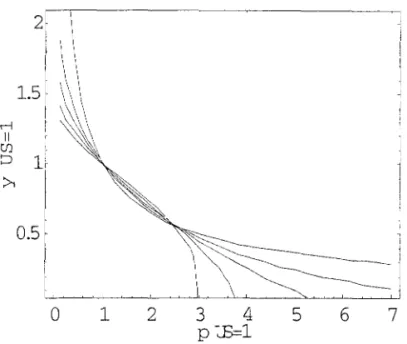

![Figure 7: Optimum time between switches and relative price of capital for (]" = 1,0.6,0.4,0.2, and O](https://thumb-eu.123doks.com/thumbv2/123dok_br/15623247.108130/55.931.255.659.138.480/figure-optimum-time-switches-relative-price-capital-o.webp)