Power and Performance Management in
Nonlinear Virtualized Computing Systems via
Predictive Control
Chengjian Wen1, Yifen Mu2*
1Department of Computer Science and Engineering, Beihang University, Beijing, China,2Key Laboratory of Systems and Control, Institute of Systems Sciences, Academy of Mathematics and Systems Science, Chinese Academy of Sciences, Beijing, China
Abstract
The problem of power and performance management captures growing research interest in both academic and industrial field. Virtulization, as an advanced technology to conserve energy, has become basic architecture for most data centers. Accordingly, more sophisti-cated and finer control are desired in virtualized computing systems, where multiple types of control actions exist as well as time delay effect, which make it complicated to formulate and solve the problem. Furthermore, because of improvement on chips and reduction of idle power, power consumption in modern machines shows significant nonlinearity, mak-ing linear power models(which is commonly adopted in previous work) no longer suitable. To deal with this, we build a discrete system state model, in which all control actions and time delay effect are included by state transition and performance and power can be defined on each state. Then, we design the predictive controller, via which the quadratic cost function integrating performance and power can be dynamically optimized. Experi-ment results show the effectiveness of the controller. By choosing a moderate weight, a good balance can be achieved between performance and power: 99.76% requirements can be dealt with and power consumption can be saved by 33% comparing to the case with open loop controller.
1 Introduction
In large scale computing systems, like data centers, huge power has been consumed and the consumption is increasing greatly each year([1]). This gives rise to heavy pressure on environ-ment and resource. Thus performance and power manageenviron-ment has become more and more important and captured growing research attention in both industrial and academic fields.
As an advanced technology, virtualization can provide a promising approach to save power ([2]) and has become a basic architecture in most data centers today. In the virtualized systems, the services are enclosed in the virtual machines (VM). Many VMs can be hosted on one physi-cal machine (PM) and the VMs can be created or destroyed or migrated between different PMs OPEN ACCESS
Citation:Wen C, Mu Y (2015) Power and Performance Management in Nonlinear Virtualized Computing Systems via Predictive Control. PLoS ONE 10(7): e0134017. doi:10.1371/journal. pone.0134017
Editor:Yongtang Shi, Nankai University, CHINA
Received:March 17, 2015
Accepted:July 3, 2015
Published:July 30, 2015
Copyright:© 2015 Wen, Mu. This is an open access article distributed under the terms of theCreative Commons Attribution License, which permits unrestricted use, distribution, and reproduction in any medium, provided the original author and source are credited.
Data Availability Statement:All relevant data are within the paper and its Supporting Information files.
Funding:The work was supported by National Natural Science Foundation of China under Grant 61304159 and 61374168. The funders had no role in study design, data collection and analysis, decision to publish, or preparation of the manuscript.
at little cost. Then, by consolidating many VMs to few PMs, the PMs with low workload, utili-zation or frequency can be shut down and power consumption can be reduced. Hence, in the virtualized computing systems, more control actions is feasible, including turning on/off the PMs, turning on/off the VMs, migrating the VMs between PMs, regulating the frequency of processor etc.. Additionally, control actions often have time delay. For example, turning on/off the PM needs several minutes and thus will influence performance and power consumption greatly. These factors make it complicated to design sophisticated and fine control to manage performance and power consumption.
Because of the significance and difficulty, researchers have been trying to solve the problem from different aspects. Usually, the first step is to build a model of energy consumption(called power model below for simplicity). In the literature, linear power model is often adopted. How-ever, modern machines show significantly nonlinear features, which can be caught from data (see Section 2). Other modelling include fuzzy model etc., see e.g. [3,4]. A review for power metering can be seen in [5]. With power model, the problem can be formulated in several ways. For example, we can maximize performance under power budget(e.g. [6]) or minimize power consumption when tracking performance or load balance between VMs (e.g. [7] ), or optimize a newly defined objective, which integrates performance, power and the balance between different machines(e.g. [3][8]).
Based on the formulations, different kinds of solutions have been proposed, see [9] for a review of energy-efficient algorithms. Next we describe several specific ways. In [3][10], the authors use reinforcement learning, and in [3] the reinforcement learning method is used together with fuzzy rule bases to achieve a defined objective, which shows robust performance improvement. In [11], the authors take advantage of the min-max and shares features inherent in virtualization technologies to allocate resources to a VM based on available resources, power costs, and application utilities. In [12], a temperature-aware workload placement is proposed in data centers. In [13], game theory is applied to formulate the problem and optimize power and performance at each level of the hierarchy while maintaining scalability.
Since it can provide a unified framework as well as rigorous controller design and can deal with dynamic and uncertain environment, control theory has been applied more and more to solve the problem. For example, in [7], the self-tuning regulator(which is an adaptive control-ler) is utilized to track performance and then optimize the energy assumption based on linear power model; in [8] the authors designs optimal controller by integrating the SLA function, and introduces a two-level control with one level being faster and the other being slower; in [14] Kalman filter is introduced to track the CPU utilizations and update the allocations of CPU resources to VMs accordingly; in [15] PID controller is proposed to manage power con-sumption and CPU utilization; in [16] MPC controller is designed; in [6] both PID controller and MPC are adopted at the same time; in [17] the authors compare effects of different control-lers and find that predictive controller performs better and has some self-learning behavior. Other recent related papers are referred to [18–22].
function (which integrates both performance and power) dynamically by searching on the fea-sible state space. During the control process, the time-varying workload is predicted using an AR model. By choosing a moderate prediction horizon, the search approach becomes feasible. Experiment results validate effectiveness of the controller: by choosing a moderate weight, per-formance requirement can be satisfied for more than 99% times; meanwhile, the power con-sumption can be saved by 33% compared to the system without predictive controller. Part of this paper is presented in [23].
The paper is organized as follows. After a brief review on power models, Section 2 shows novel features on energy consumption in modern machines, which make linear power model not suitable any more. Section 3 formulates the problem by building a discrete state model. Sec-tion 4 describes the design of predictive controller. SecSec-tion 5 validates the effectiveness of the controller by experiments. And finally, Section 6 concludes the paper with some remarks.
2 Novel Features on Power Consumption
2.1 Linear Power Models in the Literature
In order to save power, a suitable power model, which catches the relationship between energy consumption per time unit (power,kilo hour)) and physical parameters when running the machine, needs to be built. In the literature, linear power model is commonly adopted for sim-plicity and convenience, in which power consumption is modeled as a linear function with respect to certain system parameters, like CPU utilization, CPU frequency or number of VMs. Below we give some typical examples.
In [6], the VM’s powerPVMis assumed to bePVM=cfrequcpu, wherePVMdenotes VM’s power,ucpuis CPU utilization of the VM, andcfreqis a model parameter which is dependent on processor frequency.
In [8], the power (kilohour) is assumed to bePower=Pidle+αUcpu, wherePidledenotes the power consumption at idle state,Ucpudenotes CPU utilization andαis a parameter which is dependent on the specific machine and application.
In [24], the speed(or frequency) of the servers(GHz) is assumed to bes=sb+α(P−b),
wheresb(Hertz) denotes the speed of a fully utilized server running atbWatts,P(Watts) denotes the power allocated to the server, while the coefficientα(units ofGHz per Watt) is the
slope of the power-to-frequency curve, which can be obtained by experiment.
In [25], the processor power is modeled as an approximately linear function with respect to the DVFS level within the limited DVFS adaptation range available in real multi-core proces-sors, i.e.,cp(k) =a(f(k+ 1)−f(k)) +cp(k−1), in whichcp(k) denotes power consumption of
the entire chip in thek-th control period,f(k) denotes total aggregated frequency of all cores on the chip in thekth control period andadenotes a generalized parameter that may vary for dif-ferent chips and applications.
2.2 Nonlinear Features of New Machines
In recent years, server technology has developed swiftly, making processors more and more advanced. Along with the progress, linear power model encounters new problems, making it unable to reflect novel features of new machines, as stated below.
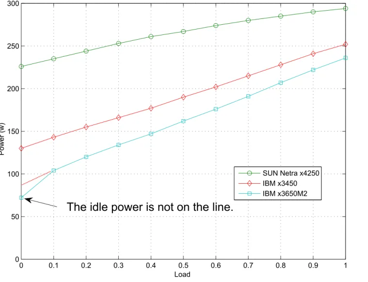
First, a significant progress is the considerable reduction of idle power. Meanwhile, other parameters, such as power at big load, do not change with it. This makes linear power model no longer accurate, as shown inFig 1.
InFig 1, power curves for the servers Sun Netra x4250 and IBM x3450 are basically in accor-dance with a line. However, for the server IBM x3650M2, the idle power is reduced signifi-cantly (from 86 to 75 in fact), which is far below the line while other points still fit with it. Apparently, linear power model is no longer suitable now and thus management based on lin-ear model is no longer optimal.
On the other hand, power saving is far from being the sole objective or even a prior objec-tive. A good performance-power ratio(performance obtained per unit of power) makes more sense, since in practice it is more important to complete a job in the given time or satisfying other requirements.
From this point of view, in a linear power model, the performance-power ratio peaks at 100% load: assume
Power¼PidleþaLoad;
then the performance-power ratio
Perf Power¼:
Load Power¼
1
aþ Pidle
Load
is a strictly increasing function with respect toLoadand peaks whenLoad= 100%.
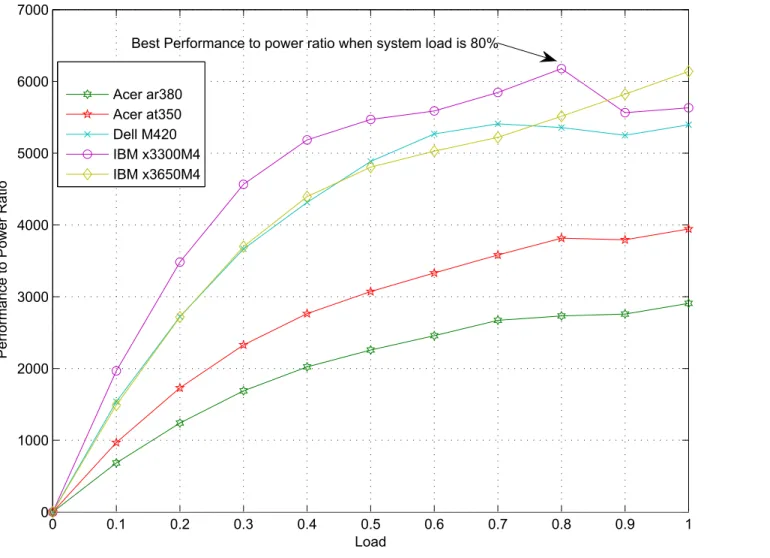
However, the real case is different for new servers, as shown inFig 2below.Fig 2draws the curve of performance-power ratio(defined as the requirements number that can be dealt with using one unit of power) with respect to load for the server IBM x3300M4 (data come from [26]).
FromFig 2, we can see that the biggest performance-power ratio occurs when the load is nearly 80% for some servers. Apparently, linear power model is not suitable any more and if we still use linear power model to simulate a modern server, we will miss the best choice. To deal with this, we will build a discrete-state-based power model in next section, which can include these nonlinear features.
3 Discrete State Model
In a virtualized computing system, there are some physical machines(PMs), denoted byPMi,
i= 1,2, ...,n, which are homogeneous or heterogeneous. Virtual machines(VMs) are hosted on each PM and can be immigrated between different PMs. In this paper, we assume that at most one VM can be hosted on one processor of a PM.
Generally, the state of a PM describes whether the PM is turned on or off, the running fre-quency of its processors, and the VM number hosted on it. Thus, we define the state ofPMias
Si ¼ ½on;vms;freq;
in which the variableonis taken asonoroff, corresponding toPMibeing turned on or turned off,vmsstands for the number of VMs running onPMi, andfreqrepresents the current fre-quencies of the running processors(sofreqhere is not a scalar).
In most situations, jobs allocated to one PM has the same type. Then, all influential factors are included in the state vector of a PM to complete the job. When different jobs are allocated to a PM, more factors, such as the architecture among the cores, must be considered, which is beyond the focus of this paper.
The time varying strength of a job is calledworkloadand denoted byλ(k) at timek. Suppose
at timek, the state isSi(k), then the performance ofPMi, denoted byperfi(k), is defined to be themaximal workloadwhich can be dealt with byPMi. Obviously, if the allocated computing resource is not sufficient, it can happen thatperfi(k)<λ(k). Here we assume that a requirement
will be abandoned if it cannot be dealt with immediately, i.e., no aggregation effect exists here. On the other hand, at timek, the power consumption ofPMi, denoted bypoweri(k), also is mainly determined bySi(k). In the experiment,poweri(k) can be measured at each time.
Apparently, there is a tradeoff between high performance and low power consumption. Thus in practice, we usually aim to get a good balance between them. To this end, we will build a discrete state model of the system and then design predictive controller.
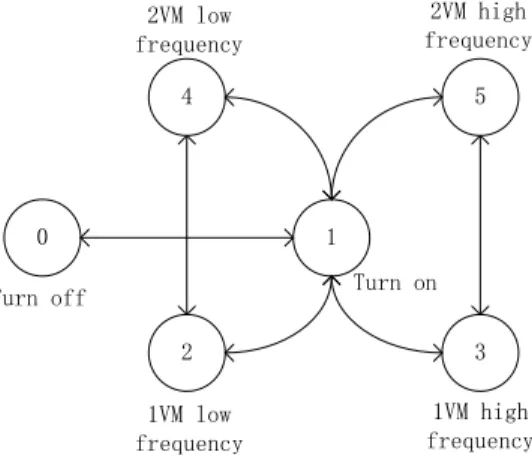
To simplify but without loss of generality, we describe the discrete model as we do in experi-ment. Let ForPMi,Si= [on,vms,freq] to be discrete and taken out of the following 6 typical values:
s0¼ ½off;0;null;s1¼ ½on;0;null;
s2¼ ½on;1;1VM on low frequency;s3 ¼ ½on;1;1VM on high frequency;
s4¼ ½on;2;2VMs both on low frequency;s5¼ ½on;2;2VMs both on high frequency
which are abbreviated asTurn off,Turn on, 1VM low frequency, 1VM high frequency, 2VM low frequency, 2VM high frequencyrespectively. Then, by regulating resource, one state can be transformed to another, as shown inFig 3, in which each directed line represents a transition between the states with positive time delay. Transition without time delay, such as the transi-tion betweens2ands3, betweens4ands5, are omitted in thefigure.
Now, assume that a jobJis hosted on some PMs. Then, the performance and power at time
kis defined on the state as
perfiJJ
iðkÞ ¼ functionðSiðkÞÞ 2 ff
JðsqÞ;q¼0;1; :::;5g; ð1Þ
poweriJJ
iðkÞ ¼ functionðSiðkÞÞ 2 fg
JðsqÞ;q¼0;1; :::;5g: ð2Þ
In practice, the value ofperfJ
For a system withnPMs, define the performance and power at timekas
perfðkÞ ¼X n
i¼1
perfiðkÞ; ð3Þ
powerðkÞ ¼ X n
i¼1
poweriðkÞ; ð4Þ
which are reasonable in view of the meanings ofperfi(k) andpoweri(k). There are several advantages of the discrete state model
1. By defining discrete states and transition between them, turning on/off a PM can be treated as a control action. To be specific,s0tos1stands for turning on the machine and the reverse stands for turning it off.
2. The idle state is also included in the model by states1, and thus it can be taken into account. Accordingly, the performance-power ratio is hidden in the model naturally and can be reflected in the cost function. Thus the discrete state model overcomes the drawbacks of lin-ear power model and is suitable for new servers.
3. Time delay effect, which exists during turning on/off a PM, now is taken into consideration. Time delay effect were often neglected in the literature, partly because it is hard to add into the model, partly because the PMs are always turned on in the past. Here, by modelling the system state discretely, time delay can be studied in a straight way.
In fact, the state transition graph builds a Markovian chain between states. This property, together with time delay effect, leads us to design predictive controller to regulate resources.
Finally, we note that this model is a coarse approximation to the real nonlinear relationship between performance, power and the system resource allocation. Putting it in a broader back-ground, the method is commonly used to deal with a significantly nonlinear function. In the future, it is necessary and possible to make fine solution in which the frequency of each proces-sor, the share of each virtual CPU, the memory and computing load will be added into the state.
4 Model based Predictive Controller
4.1 Controller Design
As we reviewed in Section 1, performance and power management problem can be handled in different ways: we can minimize power consumption under performance requirement, or we can maximize the performance within energy budget. Here we will define a quadratic cost function which combines performance and power together. By optimizing the cost function, we try to get a good balance between performance and power. To take time delay effect into consideration, the cost function must cover a time interval, which acquires the controller to predict the state for several time steps. The model predictive controller can just fit our scenario, see [24][25] for more introduction on the theory and applications of MPC.
Define the cost function at timekas below:
costðkÞ ¼ costðSðkÞ;uðk þ1Þ; :::;uðkþ PÞÞ
≜X
P
j¼1
kperfðk þjjkÞ l^ðkþjÞ k2
Qj þ
XM
j¼1
kpowerðkþ jjkÞ k2
Rj
≜X
P
j¼1
kperfð^S þ ðk þjÞjSðkÞÞ ^lðkþjÞ k2
Qj þ
XM
j¼1
kpowerð^S þ ðk þjÞjSðkÞÞ k2
Rj ð5Þ
wherej= 1, ...P,P>0 is prediction horizon, 0<MPis control horizon,u(k+j) is a feasible
control action at timek+j;^lðkþjÞis predicted workload at timek+j;^SðkþjÞis predicted state at timek+jaccording toFig 3if the control actions are take asu(k+1),...,u(k+j) sequen-tially from the stateS(k);perf(k+jjk) andpower(k+jjk) are predicted performance and power at timek+j;QjandRjare the weights(matrices ifperf(k+jjk) andpower(k+jjk) are vectors) between performance and power. Note that here we assume that there is only one PM and omit the subscriptiinSi(k),perfi(k),poweri(k).
InEq (5), the first part represents the quality of performance.^lðkþjÞ, the prediction of workload, is the required performance at timek+j. Because of time delay and uncertainty, it is possible that current control cannot create the desired effect immediately. Therefore, the differ-ence perfðkþjjkÞ ^lðkþjÞcan be treated as performance tracking error. And the quadratic termkperfðkþjjkÞ ^lðkþjÞk2
Qjis the error with weightQj.kpowerðkþjjkÞk
2
Rjis the
power value with its weightRj. Herepower(k+jjk) contains the switching cost caused by time delay. For example, the idle power is actually included inEq (5). The largerQjand smallerRj mean that the controller cares performance more, and vice versa. Obviously, appropriate choice ofQjandRjis significant for control, otherwise it cannot lead to a good balance between performance and power. This point will be discussed in Section 5 with more details.
The predictive controller aims to minimize the cost function at each time while state transi-tion graph defines constraints for control actransi-tionu(k+j):
min
fuðkþ1Þ;::;uðkþPÞgcostðkÞ;
subject to thatuðkþjÞ;j ¼ 1; :::;P;coincidesFig:3
ð6Þ
and it works as below. At each timek, the system stateS(k) now is known. Then by choosing control action sequenceu(k+ 1),...,u(k+P), a predictive controller can predict the virtual state path^Sðkþ1Þ; :::;^SðkþPÞin the futurePsteps according to the state model, i.e.Fig 3. Differ-ent control sequenceu(k+ 1),...,u(k+P) will lead to different state path^Sðkþ1Þ; :::;^SðkþPÞ,
defined above, the optimal state path can be found and thus the optimal control sequence can be determined. Then, the optimal control actionu(k+ 1),...,u(k+M),MP, in the futureM
steps can be determined, which will be adopted byPMat timek.
When there are more jobs and more machines, performance and power inEq (5)can be defined as a vector. ThenQjandRjare weight matrices and the element implies the weight between each job and each machine, which makes the calculation ofcost(k) more complicated. However, the predictive controller can be designed in a similar way.
4.2 Prediction for Workload
From description above, prediction of future workload^lðkþjÞis needed for the controller to optimize the cost function. Here we assume that workload cannot wait and accumulate, thus its prediction is independent of controller. There are certain statistical models in the literature, in which the typical ones are ANOVA and AR model, or models combined with them. We refer to [17] for more details.
Briefly speaking, ANOVA model is suitable to analyze data for long time which have repeat-able pattern, while AR model is suitrepeat-able for prediction of data for shorter time. Since we only need the instant prediction and do not focus on data’s pattern, we will apply the AR(Auto-Regression) model to predict workload in this paper.
For a sequence {x(k)}, an AR model with orderr, simplified as AR(r) model, is to utilize lin-ear combination of history data to fit the sequence and predict future values, i.e., to assume that
^
xðkÞ ¼
X
ri¼1
aixðk iÞ þek
whereekis noise and parametersaican be estimated off line or online.
ByEq (5), at each timek, we need to get the prediction^lðkþ1Þ; :::;^lðkþPÞ. Taker= 2 in the model as an example. Then we have
^ lðkÞ ¼a
1lðk 1Þ þa2lðk 2Þ:
The parametersa1,a2can be estimated by datafitting offline from history data. Then, at time
k+ 1, suppose we haveλ(1), ...λ(k), predictions for the futurePsteps are obtained by
^
lðkþ1Þ ¼a1lðkÞ þa2lðk 1Þ; ^
lðkþ2Þ ¼a
1^lðkþ1Þ þa2lðkÞ; ::::::
^
lðkþPÞ ¼a
1l^ðkþP 1Þ þa2l^ðkþP 2Þ
ð7Þ
in the order.
4.3 Optimization
At timek, suppose that we have predicted the future workload, we are at the place to choose control action sequenceu(k+1),...,u(k+P) to solve theEq (6), i.e., to optimizecost(k). Still the workload is assumed to be abandoned if it is not dealt with at current time. Note that the opti-mization can not be finished directly by a Matlab function, as [18] did.
taken from 6 different values, so the state space forPtimes has a volume of 6P, which will increase exponentially with state number and thus will be very huge when there are many states of a PM or CPU.
However, in the scenario of this paper, the state transition must satisfy physical constraints, which causes thatFig 3is not a complete digraph andu(k+ 1) can only be transited to certain states. This will shrink the state space greatly. On the other hand, considering the performance requirement in practice, the control actions which are far from being able to satisfy perfor-mance requirement, will also be abandoned first.
In this paper, we will search on the state space in the futurePtimes. Then performance and power and thus the cost functioncost(k) for each state path in the prediction horizon can be calculated according to the model. By choosing the path with minimal cost function, we can determine the control actions for the futureMtimes.
Remark 4.1:For optimizationEq (6), another feasible sophisticated approach is to use dynamic programming. To do this, we need to draw the state transition graph for futureP
steps originating from current state, which is actually a tree. When the state space is huge and
Pis big, dynamic programming might be computationally efficient.
Remark 4.2:For large scale computing systems covering a large number of processors, e.g., more than 1000, the state space will amplify sharply which will result in great challenge on search algorithms. To deal with this, the usual method is to compute off line based on history data. On the other hand, there are often several batches of homogeneous machines in real sys-tems, which can also simplify the problem highly by coarse grained modelling. Surely this brings about another tradeoff between coarse grained and finer grained modelling, which actu-ally is a tradeoff between high-cost-optimal-outcome and low-cost-suboptimal-outcome.
5 Experiment Validation
In this section, experiments will be implemented to check the effectiveness of the predictive controller based on the discrete state model.
5.1 Test Bed
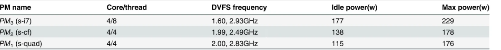
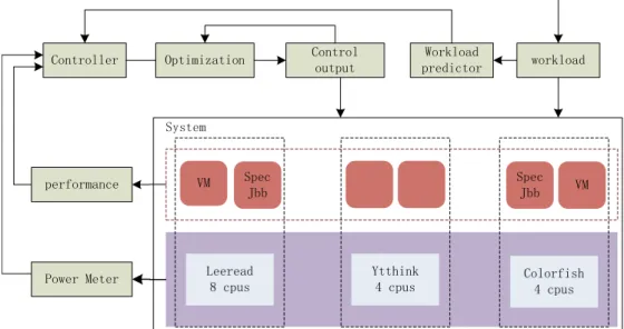
We will taken= 3,m= 2, i.e., the system is composed of 3 physical machinesPM1,PM2,PM3, and at most 2 virtual machines can be hosted on each physical machine. Configuration of the PMs are listed inTable 1.
The processors ofPM1,PM2,PM3are Core i7, Xeon 5320, Core 2 Quad respectively, the OS is Fedora 16, and the virtualization software is KVM. Note that these PMs or processors are chosen to be different, which can happen usually in practice. The heterogeneity on PMs or pro-cessors can be easily handled in the experiment by choosing appropriate parameters in perfor-mance and power models; we will see that they will not influence the effectiveness of our controller, which implies extendibility of the method.
The parameters pertinent to performance and power during control process are measured from chosen servers and listed inTable 2below, in which it is set 1T= 5min, and perf, freq are abbreviations for performance, frequency.
Table 1. Configuration of physical machines.
PM name Core/thread DVFS frequency Idle power(w) Max power(w)
PM3(s-i7) 4/8 1.60, 2.93GHz 177 229
PM2(s-cf) 4/4 1.99, 2.49GHz 138 178
PM1(s-quad) 4/4 2.00, 2.83GHz 115 176
Then the flow chart with predictive controller in the virtualized computer system is drawn inFig 4.
The data of workload in our experiment can be seen inS1 File.
5.2 Choice of Control Parameters
By the definition ofcost(k) inEq (5), four parameters will influence its value: the integersP,M
and the weightsQ,R. Hence, they will influence the solution of optimizationEq (6)and thus the effect of controller. Additionally,P,Minfluence complexity of the problem more heavily whileQ,Rwill influence the choice of control actions more significantly.
Now, we decide the prediction and control horizonPandMfirst. As we have stated above, long prediction horizon will lead to exponentially increasing search space for predicted state, which is not bearable for large scale servers. SoPcannot be very large. On the other hand,P
must be chosen according to the characteristics of workload so that prediction accuracy can be assured. With deeper prediction steps, prediction of workload will become less accurate. Based on these points, we takeP= 3 in the experiment.Mis taken as 1 as in the literature to avoid the conflict between control actions at timekandk+ 1.
Then, we decide the weightsQjandRj. First, we setQj= 1,j= 1,2, ...,P, by which we mean that the cost resulting from performance tracking at each time are the same.
As to the power saving weightR(denoted byRsinceM= 1), it is important to choose a mod-erate value for it: differentRleads to different cost function and thus different optimal control
Table 2. Parameters of control actions about performance and power.
Possible control action Time delay Power Perf delay
turning off a PM 1T max power 0
turning on a PM 2T max power 0
changing freq by DVFS 0 determined by current freq determined by new freq
turning on a VM 1T power after VM turning on 0
turning off a VM 0 power before VM turning down 0
VM immigration 0 determined by new PM determined by new PM
doi:10.1371/journal.pone.0134017.t002
action, and then different performance quality and power consumption. Moreover, it can be imagined that a moderate value ofRis dependent of jobs’types. In the experiment, we will choose differentRfor an identical workload sequence, and compare the results under eachR.
5.3 Experiment Results
To test the effectiveness of predictive controller, we will compare performance and power of the system under control with the case without controller(or equally, with open loop control-ler). For the system with predictive controller, we will compare experiment results under differ-ent choice ofR.
When the system is managed without controller, all physical machines will be always turned on so as to guarantee the performance requirement, thus turning on/off a PM is not an option of control actions in this case. This is just the practice for many data centers today.
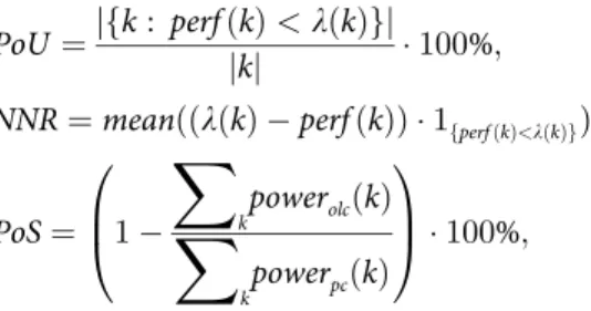
We define several criteria as below:
PoU¼jfk: perfðkÞ<lðkÞgj
jkj 100%;
NNR¼meanððlðkÞ perfðkÞÞ 1
fperfðkÞ<lðkÞgÞ;
PoS¼ 1
X
kpowerolcðkÞ
X
kpowerpcðkÞ 0
B @
1
C
A100%;
ð8Þ
wheremean(x(k)) is average of sequencex(k),powerolc(k) is the measured power without con-troller, andpowerpc(k) is the measured power with predictive controller. It is easy to see that
PoUstands for thepercentof timesunderperformance requirement(i.e., the performance is not satisfied),NNRstands for thenumberofnon-handled-request, andPoSstands for the per-centof powersavingcompared with the open-loop-controller case.
5.3.1 Basic Results. Table 3below roughly shows the experiments results with differentR: FromTable 3, we can see that the predictive controller can save power considerably com-pared to the system with open-loop controller while the performance tracking result is very dif-ferent under difdif-ferentR. To be specific,
(1). WhenR= 5,PoUis very small, being 0.23%, meaning that the performance requirement can be satisfied for almost all the times. Averagely, 1000 requests cannot be handled at each time. However, in this case, the power can be saved only by 21%, which is not bad but can be improved still.
(2). WhenR= 50,PoUis also very small, being 0.24%, which is almost the same withR= 5 case. And now there are 3478 requests which will be abandoned at each time. On the other hand, power consumption can be saved by 33%, which is great progress toR= 5 case.
(3). WhenR= 100,PoUnow increases pretty highly, being 38%, implying that for more than one-third time, the performance requirement cannot be satisfied, which is very bad. And
Table 3. Performance and power criteria under differentR.
R PoU NNR PoS
5 0.23% 1000 21%
50 0.24% 3478 33%
100 38.00% 7911 35%
200 50.20% 11854 38%
500 74.48% 35582 51%
now the amount of requests that cannot be handled at each time is high, being 7911. At the same time, power is saved by only 35%, which is very near that ofR= 50 case.
(4). WhenR= 200,PoUnow becomes 50.2%, implying that performance cannot be satisfied for more than half of the time, while power is saved by 38%, which is still near that ofR= 50 case.
(5). WhenR= 500,PoUnow becomes 74.48%, implying a terrible performance. Power con-sumption is saved by 51%, which is a great progress to smallerR. Obviously, we cannot choose such a decision since performance is prior to power.
With respect to increasingR, results inTable 3coincide with the physical meaning ofR: withRincreasing, power saving holds a bigger weight in the cost function, and thus power sav-ing can become better, while performance becomes worse. We can find thatR= 50 is a suitable weight, which can achieve a good balance between performance tracking (99.76% requirement can be deal with) and power saving (energy consumption can be saved by 33%).
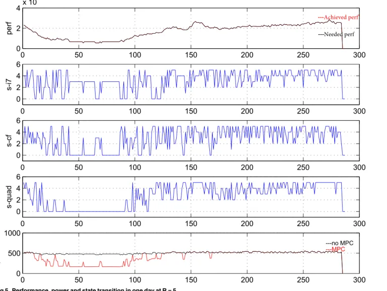
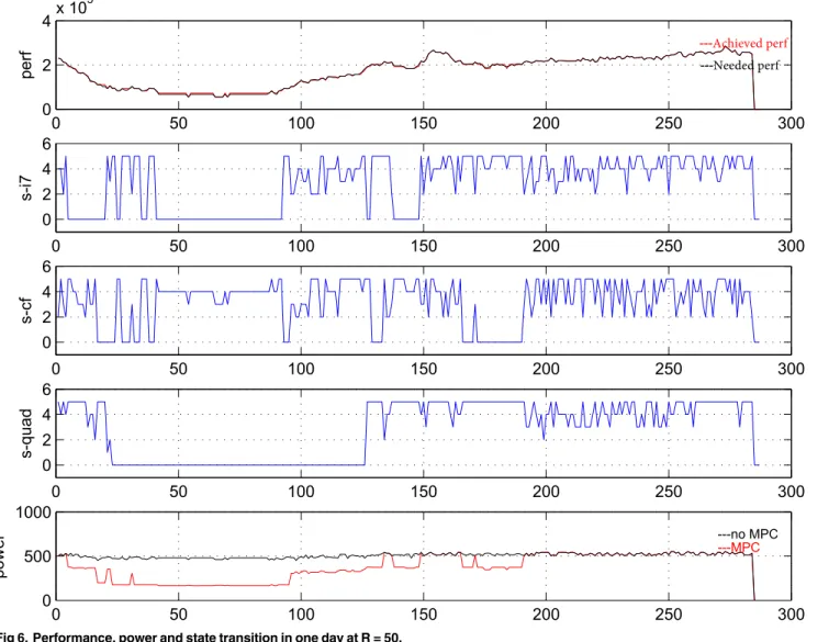
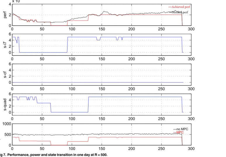
5.3.2 Control Process in Details. Next, we will present the detailed process of the predic-tive controller. To this end, curves of the state, performance and power for three PMs are shown in each ofFig 5,Fig 6,Fig 7as below, which contains five pictures in them. The data is
measured for 24 hours every 5 minutes and the weightRis taken as 5, 50, 500 respectively in three figures.
InFig 5,Fig 6,Fig 7, the horizontal axis denotes time; the vertical axis of the first picture denotes number of requirements that are coming and handled; the vertical axes of the second, third and fourth pictures denote the frequencies of three PMs; the vertical axis of the fifth pic-ture denotes total power of the system. In the first picpic-ture, black curve denotes the coming requirement while red curve denotes the handle requirement at each time. In the fifth curve, black curve denotes the power without controller while red curve denotes the power with pre-dictive controller.
From the curves, control actions can be distinguished from the change of frequencies and power clearly. When the frequency is zero and the power is smaller than the sum of idle pow-ers, we can see that PM under observation is indeed shut down. And we can also see that under open loop control, the power is always maximal.
FromFig 5,Fig 6,Fig 7, whenR= 5, the action of turning on/off the PM is used rarely, and the performance can be satisfied well while power saving is not very good. WhenR= 500, one PM is always being turned off, the power saving is good, while the performance tracking is bad.
R= 50 is a moderate choice, which can lead to a good balance between performance and power. Meanwhile, atR= 50, VMs can be migrated between PMs, and power cycling is an effective control action.
To sum up, the choice ofRis very crucial for control. IfRcan be taken moderately, such as
R= 50, then a good balance between performance and power can be achieved: on one hand, the performance can be satisfied well; on the other hand, the power consumption can be saved considerably. In practice,Rcan be obtained by learning from experience, which depends on the specific system and jobs.
6 Conclusions and Future Work
In this paper, the power saving problem in the nonlinear virtualized computing system is stud-ied. First, we present some novel nonlinear characteristics of newer servers which are found from data. Such nonlinear features make linear power model not suitable again for fine control. Then, we build a discrete system state model, in which all control actions such as turning on/ off a PM (or a VM) can be included and time delay effect can be reflected too. Then, by defin-ing a quadratic cost function which involves both performance and power, the predictive con-troller based on the discrete state model can be designed in a natural way. Thus the cost function can be optimized by regulating computing resources dynamically. Experimental
results show that with an appropriate weight of performance and power in the cost function, the predictive controller can achieve efficient performance and power management: almost 99.76% requirements can be dealt with and 33% power consumption can be saved compared with the case without controller.
In practice, the architecture of processors is also important and needs to be taken into account. Additionally, as we have noted before, the proposed discrete state model in this paper is still very rough. In order to get better effect, more sophisticated models need to be built so that more details can be included such as the share of VCPU, the frequency values of proces-sors and so on. These will be left in the future work.
Finally, new technologies have been booming in control theory, such as the theory on multi-agent systems, in which massive agents with individual dynamics are contained and the consensus or special formations are often control objectives([26][27]). It can be surprisingly correlated with distributed computation, see [28][29]. Will such theory provide some inspira-tions to problems under study in the current paper? We do not know now while it might be interesting if new relations can be built.
Supporting Information
S1 File.(XLS)
Author Contributions
Conceived and designed the experiments: CW. Performed the experiments: CW. Analyzed the data: YM. Contributed reagents/materials/analysis tools: YM. Wrote the paper: YM.
References
1. Koomey J.Growth in data center electricity use 2005 to 2010. 2011, Oakland, CA: Analytics Press. August 1. Aavailable:http://www.analyticspress.com/datacenters.html.
2. Wen CJ, He J, Zhang J, Long X. PCFS: Power Credit Based Fair Scheduler Under DVFS for Muliticore Virtualization Platform. Proceedingoint of view, in a linear power model, the ps of the 2010 IEEE/ACM Int’l Conference on Green Computing and Communications & Int’l Conference on Cyber, Physical and Social Computing. 2010: 163–170.
3. Vengerov D. A reinforcement learning approach to dynamic resource allocation. Journal Engineering Applications of Artificial Intelligence. 2007, 20(3): 383–390. doi:10.1016/j.engappai.2006.06.019
4. Xu J, Zhao M, Fortes J, Carpenter R, Yousif M. On the use of fuzzy modeling in virtualized data center management. Proceedings of the IEEE Int’l Confonrefence on Autonomic Computing 2007. 2007: 25ï ¿½C35. 10.1109/ICAC.2007.28.
5. Krishman B, Amur H, Gavrilovska A, Schwan K. VM power metering: feasibility and challenges. ACM SIGMETRICS Performance Evaluation Review archive. 2010, 38(3): 56–60. doi:10.1145/1925019. 1925031
6. Lim H, Kansal A, Liu J. Power Budgeting for Virtualized Data Centers. Proceedings of the 2011 USE-NIX conference on USEUSE-NIX annual technical conference. 2011: 5–15.
7. Wen CJ, Long X, Mu YF. Adaptive Controller for Dynamic Power and Performance Management in the Virtualized Computing Systems. PLoS ONE. 8(2): e57551. 10.1371/journal.pone.0057551. doi:10. 1371/journal.pone.0057551PMID:23451241
8. Kusic D, Kephart JO, Hanson JE, Kandasamy N, Jiang GF. Power and Performance Management of Virtualized Computing Environments Via Lookahead Control. Journal Cluster Computing. 2009, 12(1): 1–15. doi:10.1007/s10586-008-0070-y
9. Albers S. Energy-efficient algorithms. Communications of the ACM. 2010: 53(5): 86–96. doi:10.1145/ 1735223.1735245
11. Cardosa M, Korupolu MR, Singh A. Shares and utilities based power consolidation in virtualized server environments. Proceedings of the 11th IFIP/IEEE International Symposium on Integrated Network Management. 2009: 327–334. doi:10.1109/INM.2009.5188832
12. Moore JD, Chase J, Ranganathan P, Sharma R. Making scheduling‘cool’: temperature-aware work-load placement in data centers. Proceedings of the Annual Conference on USENIX Annual Technical Conference 2005. 2005: 5–5.
13. Khargharia B, Hariri S,Yousif MS. Autonomic power and performance management for computing sys-tems. Cluster Computing. 2008, 11(2): 167–181. doi:10.1007/s10586-007-0043-6
14. Kalyvianaki E, Charalambous T, Hand S. Self-adaptive and self-configured cpu resource provisioning for virtualized servers using kalman filters. Proceedings of the 6th International Conference on Auto-nomic Computing, ACM. 2009: 117–126.
15. Kjaer MA, Kihl M, Robertsson A. Resource allocation and disturbance rejection in web servers using SLAs and virtualized servers. IEEE Trans. Network and Service Management. 2009, 6(4): 226C239. doi:10.1109/TNSM.2009.04.090403
16. Xu CZ, Liu BJ, Wei JB. Model predictive feedback control for QoS assurance in webservers. Computer. 2008, 41(3): 66C72. doi:10.1109/MC.2008.93
17. Xu W, Zhu Xy, Singhal S, Wang Zk. Predictive Control for Dynamic Resource Allocation in Enterprise Data Centers. The 10th IEEE/IFIP Network Operations and Management Symposium, Vancouver, Canada. 2006: 115–126.
18. Wang YF, Wang XR, Chen M, Zhu XY. Power-Efficient Response Time Guarantees for Virtualized Enterprise Servers. Proceedings of the 2008 Real-Time Systems Symposium. 2008: 303–312. doi:10. 1109/RTSS.2008.20
19. Ardagna D, Trubian M, Zhang L. SLA based resource allocation policies in autonomic environments. Journal of Parallel and Distributed Computing. 2007, 67(3): 259–270. doi:10.1016/j.jpdc.2006.10.006
20. Raghavendra R, Ranganathan P, Talwar V, Wang ZK, Zhu XY. No power struggles: Coordinated multi-level power management for the data center. ACM SIGARCH Computer Architecture News. 2008, 36 (1): 48–59. doi:10.1145/1353534.1346289
21. Govindan S, Choi J, Urgaonkar B, Sivasubramaniam A, Baldni A. Statistical profiling-based techniques for effective power provisioning in data centers. Proceedings of the 4th ACM European Conference on Computer Systems. 2009: 317–330.
22. Kusic D,Kandasamy N, Jiang GF. Combined power and performance management of virtualized com-puting environments serving session-based workloads. IEEE Transactions on Network and Service Management. 2011, 8(3): 245–258. doi:10.1109/TNSM.2011.0726.100045
23. Wen CJ, Long X, Mu YF. Power and performance management via model predictive control for virtua-lized cluster computing. Proceedings of the 32nd Chinese Control Conference. 2013: 2591–2596.
24. Gandhi A, Harchol-Balter M, Das R, Lefurgy C. Optimal power allocation in server farms. Proceedings of the 11th International Joint Conference on Measurement and Modeling of Computer Systems, ACM. 2009: 157–168.
25. Ma K, Li X, Chen M, Wang XR. Scalable power control for many-core architectures running multi-threaded applications. ACM SIGARCH Computer Architecture News. 2011, 39(3): 449–460. doi:10. 1145/2024723.2000117
26. Standard Performance Evaluation Corporation. The SPEC Powerssj2008 benchmark. available:http:// www.spec.org/power_ssj2008/results/res2010q4/power_ssj2008-20100921-00294.html
27. Richalet J. Industrial applications of model based predictive control. Automatica. 1993, 29(5): 1251–
1274. doi:10.1016/0005-1098(93)90049-Y
28. Qin SJ, Badgwell TA. A survey of industrial model predictive control technology. Control Engineering Practice. 2003, 11: 733C764. doi:10.1016/S0967-0661(02)00186-7
29. Wang L, Chen ZQ, Liu ZX, Yuan ZZ. Finite time agreement protocol design of multi-agent systems with communication delays. Asian Journal of Control. 2009, 11(3):281–286. doi:10.1002/asjc.104
30. Wang L, Sun SW, Xia CY. Finite-time stability of multi-agent system in disturbed environment. Nonlin-ear Dynamics. 2012, 67(3): 2009–2016. doi:10.1007/s11071-011-0125-0
31. Tsitsiklis JN, Bertsekas DP, Athans M. Distributed asynchronous deterministic and stocahstic gradient optimization algorithms. IEEE Transactions on Automatic Control. 1986, 31(9): 803C812. doi:10.1109/ TAC.1986.1104412