ISSN 0101-8205 / ISSN 1807-0302 (Online) www.scielo.br/cam
Bézier control points method to solve constrained
quadratic optimal control of time varying linear systems
F. GHOMANJANI, M.H. FARAHI and M. GACHPAZAN Department of Applied Mathematics, Faculty of Mathematical Sciences
Ferdowsi University of Mashhad, Mashhad, Iran E-mail: [email protected]
Abstract. A computational method based on Bézier control points is presented to solve optimal control problems governed by time varying linear dynamical systems subject to terminal state equality constraints and state inequality constraints. The method approximates each of the system state variables and each of the control variables by a Bézier curve of unknown control points. The new approximated problems converted to a quadratic programming problem which can be solved more easily than the original problem. Some examples are given to verify the efficiency and reliability of the proposed method.
Mathematical subject classification: 49N10.
Key words:Bézier control points, constrained optimal control, linear time varying dynamical systems.
1 Introduction
In the numerical solution of differential equations, polynomial or piecewise polynomial functions are often used to represent the approximate solution [1]. Legendre and Chebyshev polynomials are used for solving optimal control prob-lems (see [2], [3], [4] and [5]). Razzaghi and Yousefi [6] defined functions which they called Legendre wavelets for solving constrained optimal control problem. In particular, B-splines and Bezier curves have become popular tools for solving dynamical systems [7]. For both Bezier and B-spline representations, the curve
or surface shape is outlined by a “control polygon” that is formed by connecting the control points. Since the control point structure captures important geometric features of the Bezier or B-spline shape, it is tempting to perform computations just based on the control points. This paper intends to investigate the use of the control points of Bezier representations for solving optimal control problems with inequality constrained. Since the use of B-splines is to cause the continuity of control curves, we propose to represent the approximate solution in Bezier curves for time varying optimal control problem with inequality constraints. The choice of the Bezier form rather than the B-spline form is due to the fact that the Bezier form is easier to symbolically carry out the operations of multiplication, composition and degree elevation than the B-spline form. We choose the sum of squares of the Bezier control points of the residual to be the measure quantity. Minimizing this quantity gives the approximate solution. Obviously, if the quan-tity is zero, then the residual function is also zero, which implies the solution is the exact solution. We call this approach the control-point-based method.
Consider the following time varying optimal control problem with pathwise state inequality constraints,
min Cost= 1
2x(tf)
TH
(tf)x(tf)+
Z tf t0
xTPx+uTQu+Kx+Rudt
s.t. ˙
x(t)= A(t)x(t)+B(t)u(t)+F(t), x(t0)=x0,
li(x(tf))=0, i∈ E = {1,2, . . . ,N1},
gh(x(tf))≤0, h∈ I = {1,2, . . . ,N2},
q(t,x(t))≤0, t ∈ [t0,tf], (1)
where
H(t)= [hi j(t)]p×p, P(t)= [pi j(t)]p×p, Q(t)= [qi j(t)]m×m, A(t)= [ai j(t)]p×p and B(t)= [bi j(t)]p×m
are matrices functions andK(t)=(k1(t) . . . kp(t)),R(t)=(r1(t) . . . rm(t)), F(t) = (f1(t) . . . fp(t))T are vectors functions, where the entries of
mentioned matrices are not polynomials in[t0,tf], Taylor series is used for
ap-proximation. x(t) = (x1(t) x2(t) . . . xp(t))T ∈ Rp is p×1 trajectory state
vector,u(t)∈U= {(u1(t)u2(t) . . . um(t))T :bi−(t)≤ui ≤ bi+(t), 1≤ i ≤
m} ⊆ Rm ism×1 control vector. The fixed finite terminal time tf is given,
andx0 is the vector of initial conditions. In addition,li : Rp → R fori ∈ E, gh : Rp → Rforh ∈ I,q : [t0,tf] ×Rp → R, andb−i (t),b
i
+(t), 1 ≤i ≤ m are given bounded functions.
The constrained optimal control of a linear system with a quadratic perfor-mance index has been of considerable concern and is well covered in many pa-pers (see [6] and [8]). One of the methods to solve constrained optimal control problem(1), based on parameterizing the state/control variables, which convert
the problem to a finite dimensional optimization problem, i.e. a mathematical programming problem (see [9], [10], [11]-[16]).
Analytical techniques developed in [5] are of benefit also in studying the convergence properties of related algorithms for solving optimal control prob-lems, involving Chebyshev type functional constraints where, owing to the use of a variable step-size in integration or high order integration procedures, it is either not possible or inconvenient to base the analysis on an a priori dis-cretization of the dynamic. The method used slack variables to convert the inequality constraints into equality constraints. This approach has an obvi-ous disadvantage when applied to constrained optimal control of time vary-ing linear problems because it converts the linear constraints into a nonlinear one (see [17]).
In this paper, we show a novel strategy by using the Bézier curves to find the approximate solution for(1). In this method, we divided the time interval,
intoksubintervals and approximate the trajectory and control functions in each
subinterval by Bézier curves. We have chosen the Bézier curves as piecewise
polynomials of degreen, and determine Bézier curves on any subinterval by
n+1 control points. By involving a least square optimization problem, one can
find the control points, where the Bézier curves that approximate the action of control and trajectory, can be found as well (see [7] and [18]).
2 Least square method
Letkbe a chosen positive integer and{t0 <t1 <∙ ∙ ∙<tk =tf}be an
equidis-tance partition of[t0,tf]with lengthτ andSj = [tj−1,tj]for j = 1,2, . . . ,k.
We define the following suboptimal control problems
min Costj =Cj k +
Z tj tj−1
xTj Pxj+uTjQuj+Kxj+Ruj
dt
s.t. ˙
xj(t)=A(t)xj(t)+B(t)uj(t)+F(t), x1(t0)=x0, t ∈ Sj, li(xk(tf))=0, i ∈ E,
gh(xk(tf))≤0, h∈ I,
q(t,xj(t))≤0, t∈ Sj,j =1,2, . . . ,k, (2)
where Cj k = 12δj kxTk(tf)H(tf)xk(tf), and δj k is the Kronecker delta which
has the value of unity when j =k and otherwise is zero.
xj(t)= x1j(t)x2j(t) . . . xpj(t)
T
and uj(t)= u1j(t)u2j(t) . . . umj(t)
T
are respectively vectors ofx(t)andu(t)when are considered inSj = [tj−1,tj].
Our strategy is using Bezier curves to approximate the solutions xj(t) and
uj(t)byvj(t) andwj(t)respectively, wherevj(t)andwj(t)are given below.
Individual Bezier curves that are defined over the subintervals are joined together to form the Bezier spline curves. For j =1,2, . . . ,k, define the Bezier
poly-nomials of degree n that approximate the actions of xj(t) anduj(t) over the
intervalSj = [tj−1,tj]as follows:
vj(t)= n
X
r=0 arjBr,n
t−tj−1 τ
,
wj(t)= n
X
r=0 brjBr,n
t−tj−1 τ
,
(3)
where
Br,n
t−tj−1 τ
=
n r
1
τn(tj −t) n−r
is the Bernstein polynomial of degreen over the interval[tj−1,tj], a j
r andb
j r
are respectively p andm ordered vectors from the control points. By
substi-tuting (3) in (2), one may define residual R1,j(t)and R2,j(t)fort ∈ [tj−1,tj]
as:
R1,j(t)= ˙vj(t)−A(t)vj(t)−B(t)wj(t)−F(t),
R2,j(t)=vTj(t)P(t)vj(t)+wTj(t)Q(t)wj(t)+K(t)vj(t)+R(t)wj(t).
(4)
Beside the boundary conditions onv(t), in nodes, there are also continuity
con-straints imposed on each successive pair of Bezier curves. Since the differential equation is of the first order, the continuity of x (or v) and its first derivative
gives
v(s)j (tj)=v(s)j+1(tj), s =0,1, j =1,2, . . . ,k−1.
wherev(s)j (tj)is thes-th derivative ofvj(t)with respect totatt=tj.
Thus the vector of control pointsarj (forr =0,1,n−1 andn) must satisfy
anj tj −tj−1n =a0j+1 tj+1−tj
n , anj −anj−1 tj −tj−1n−1= a1j+1−a
j+1 0
tj+1−tj
n−1 .
(5)
One may recall that arj is an p ordered vector. This approach is called the
subdivision scheme (or τ-refinement in the finite element literature), in the
Section 3, we prove the convergence in the approximation with Bezier curves whenntends to infinity.
Note 1: If we consider theC1continuity ofw, the following constraints will
be added to constraints (5),
bnj tj −tj−1n=b0j+1 tj+1−tj
n , bnj −bnj−1
tj −tj−1n−1= b1j+1−b
j+1 0
tj+1−tj
n−1 ,
(6)
where the so-calledbrj is anmordered vector.
Now, we define residual function inSj as follows
Rj =(Cj k)2+
Z tj tj−1
wherek.kis the Euclidean norm (Recall that R1,j(t)is a pvector wheret∈ Sj)
andMis a sufficiently large penalty parameter. Our aim is to solve the following
problem overS=Sk
j=1Sj,
min
k
X
j=1
Rj
s.t.
li(vk(tk))=0, i ∈ E, gh(vk(tk))≤0, h ∈ I,
q(t,vj(t))≤0, t ∈Sj, j =1,2, . . . ,k,
v(s)j (tj)=v (s)
j+1(tj), s =0,1, j=1,2, . . . ,k−1. (7)
The mathematical programming problem (7) can be solved by many subroutines, we used Maple 12 to solve this optimization problem.
Note 2: If in time varying optimal control problem (1),x(tf)be unknown, then
we setCkk =0.
Note 3: To find good polynomial approximation, one needs to increase the
degree of polynomial, in this article, we used sectional approximation, to find accurate results by low degree polynomials.
3 Convergence analysis
In this section, we analyze the convergence of the control-point-based method when applied to the following time varying optimal control problem:
min I = 1
2x(1)H(1)x(1)+
Z 1 0
(x(t)P(t)x(t)+u(t)Q(t)u(t) + K(t)x(t)+R(t)u(t))dt
s.t.
where the statex(t) ∈ R,u(t) ∈ R,a,b ∈ R, H(t), P(t), Q(t), K(t), R(t),
A(t),B(t)andF(t)are polynomials in[0,1].
Without loss of generality, we consider the interval [0,1]instead of [t0,tf],
since one can change the variabletwith the new variablezbyt=(tf−t0)z+t0
wherez ∈ [0,1].
Lemma 3.1. For a polynomial in Bezier form
x(t)=
n1
X
i=0
ai,n1Bi,n1(t),
we have
Pn1
i=0ai,n2 1
n1+1 ≥
Pn1+1
i=0 ai,n2 1+1
n1+2
≥. . .≥
Pn1+m1
i=0 a2i,n1+m1
n1+m1+1 ,
where ai,n1+m1 is the Bezier coefficients of x(t) after it is degree-elevated to
degree n1+m1.
Proof. See [1].
The convergence of the approximate solution could be done in two ways.
1. Degree raising case of the Bezier polynomial approximation. 2. Subdivision case of the time interval.
In the following we prove the convergence in each case.
3.1 Degree raising case
Theorem 3.2. If time varying optimal control problem (8) has a unique, C1 continuous trajectory solution x, Cˉ 0 continuous control solution u, then theˉ approximate solution obtained by the control-point-based method converges to the exact solution as the degree of the approximate solution tends to infinity.
Proof. Given an arbitrary small positive number ǫ > 0, by the Weierstrass
Theorem (see[19]) one can easily find polynomials Q1,N1(t)of degree N1and
Q2,N2(t)of degreeN2such that
kd
iQ
1,N1(t)
dti −
dixˉ(t) dti k∞≤
ǫ
16,i =0, 1, and kQ2,N2(t)− ˉu(t)k∞≤
ǫ
wherek.k∞stands for theL∞-norm over[0,1]. Especially, we have
ka−Q1,N1(0)k∞≤
ǫ
16,
kb−Q1,N1(1)k∞≤
ǫ
16,
ka1−Q2,N2(0)k∞≤
ǫ
16. (9)
In general, Q1,N1(t)and Q2,N2(t)do not satisfy the boundary conditions. Af-ter a small perturbation with linear and constant polynomials αt +β and γ,
respectively for Q1,N1(t)and Q2,N2(t), we can obtain polynomials P1,N1(t) =
Q1,N1(t)+(αt+β)andP2,N2(t)=Q2,N2(t)+γ such thatP1,N1(t)satisfy the boundary conditions P1,N1(0) = a, P1,N1(1) = b, and P2,N2(0) = a1. Thus
Q1,N1(0)+β =a, andQ1,N1(1)+α+β =b. By using (9), one have
ka−Q1,N1(0)k∞= kβk∞≤
ǫ
16,
kb−Q1,N1(1)k∞= kα+βk∞≤
ǫ
16. Since
kαk∞− kβk∞≤ kα+βk∞≤
ǫ
16, so
kαk∞≤
ǫ
16+ kβk∞≤
ǫ 16 + ǫ 16 = ǫ 8. By the time,a1= P2,N2(0)= Q2,N2(0)+γ, so
ka1−Q2,N2(0)k∞= kγk∞≤
ǫ
16. Now, we have
kP1,N1(t)− ˉx(t)k∞ = kQ1,N1(t)+αt+β− ˉx(t)k∞
≤ kQ1,N1(t)− ˉx(t)k∞+ kα+βk∞≤
ǫ 8 < ǫ 3,
d P1,N1(t)
dt −
dxˉ(t)
dt ∞ =
d Q1,N1(t)
dt +α−
dxˉ(t)
dt ∞ ≤
d Q1,N1(t)
dt −
dxˉ(t)
dt ∞
+ kαk∞≤ 3ǫ
16 <
ǫ
kP2,N2(t)− ˉu(t)k∞ = kQ2,N2(t)+γ − ˉu(t)k∞
≤ kQ2,N2(t)− ˉu(t)k∞+ kγk∞≤
ǫ
8 <
ǫ
3. Now, let define
L PN(t)=L P1,N1(t),P2,N2(t),P˙1,N1(t)
= d P1,N1(t)
dt −A(t)P1,N1(t)−B(t)P2,N2(t)=F(t),
for everyt ∈ [0,1]. Thus forN ≥ max{N1,N2}, one may find an upper bound
for the following residual:
kL PN(t)−F(t)k∞ = kL(P1,N1(t),P2,N2(t),P˙1,N1(t))−F(t)k∞
≤
d P1,N1(t)
dt −
dxˉ(t)
dt
∞
+kA(t)k∞kP1,N1(t)− ˉx(t)k∞
+ kB(t)k∞kP2,N2(t)− ˉu(t)k∞
≤ C1 ǫ
3+
ǫ
3+
ǫ
3
=C1ǫ
whereC1=1+ kA(t)k∞+ kB(t)k∞is a constant.
Since the residualR(PN):=L PN(t)−F(t)is a polynomial, we can represent
it by a Bezier form. Thus we have
R(PN):= m1
X
i=0
di,m1Bi,m1(t).
Then from Lemma 1 in [1], there exists an integer M(≥ N) such that when
m1> M, we have
1
m1+1
m1
X
i=0
di,m2 1− Z 1
0
(R(PN))2dt
< ǫ,
which gives
1
m1+1
m1
X
i=0
di,m2 1 < ǫ+ Z 1
0
Supposex(t)andu(t)are approximated solution of (8) obtained by the
control-point-based method of degreem2(m2≥m1≥ M). Let
R(x(t),u(t),x˙(t)) = L(x(t),u(t),x˙(t))−F(t) =
m2
X
i=0
ci,m2Bi,m2(t), m2≥m1≥ M, t ∈ [0,1]. Define the following norm for difference approximated solution(x(t),u(t))and
exact solution(xˉ(t),uˉ(t)):
k(x(t),u(t))−(xˉ(t),uˉ(t))k := Z 1
0 1 X
j=0
djx(t) dtj −
djxˉ(t) dtj
2
dt
+ Z 1
0
|u(0)− ˉu(0)|dt.
(11)
It is easy to show that:
k(x(t),u(t))−(xˉ(t),uˉ(t))k ≤C |x(0)− ˉx(0)| + |x(1)− ˉx(1)|
+ |u(0)− ˉu(0)| + kR(x(t),u(t),x˙(t))k22 =C
Z 1 0
m2
X
i=0
(ci,m2Bi,m2(t))
2dt
≤ C
m2+1
m2
X
i=0
c2i,m2
(12)
Last inequality in (12) is obtained from Lemma 1 in [1] in whichCis a constant
positive number. Now from Lemma 1 in [1], one can easily show that:
k(x(t),u(t))−(xˉ(t),uˉ(t))k ≤ C m2+1
m2
X
i=0
c2i,m2 ≤ C m2+1
m2
X
i=0
di,m2 2
≤ C
m1+1
m1
X
i=0
di,m2 1 ≤C(ǫ+C12ǫ2)
= ǫ1, m1≥ M,
(13)
Thus, from (13) we have:
kx(t)− ˉx(t)k ≤ǫ1, ku(t)− ˉu(t)k ≤ǫ1.
Since the infinite norm and the norm defined in (11) are equivalent, there is a
ρ1>0 where
kx(t)− ˉx(t)k∞≤ρ1ǫ1,
ku(t)− ˉu(t)k∞≤ρ1ǫ1.
Now, we show that the approximated cost function tends to exact cost function as the degree of Bezier approximation increases. Define
Iexact =
1
2xˉ(1)H(1)xˉ(1)+
Z 1 0
(xˉ(t)P(t)xˉ(t)+ ˉu(t)Q(t)uˉ(t) +K(t)xˉ(t)+R(t)uˉ(t))dt,
Iappr ox =
1
2x(1)H(1)x(1)+
Z 1 0
(x(t)P(t)x(t)+u(t)Q(t)u(t) +K(t)x(t)+R(t)u(t))dt,
fort ∈ [0,1]. Now, there are four positive integersMi ≥0,i =1, . . . ,6, such
that
kP(t)k∞≤ M1, kQ(t)k∞≤ M2, kK(t)k∞≤ M3, kR(t)k∞≤ M4, k ˉx(t)k∞≤ M5 and k ˉu(t)k∞≤ M6.
Since
kx(t)k∞− k ˉx(t)k∞≤ k ˉx(t)−x(t)k∞≤ρ1ǫ1, ku(t)k∞− k ˉu(t)k∞≤ k ˉu(t)−u(t)k∞≤ρ1ǫ1,
we have
so
k ˉx(t)+x(t)k∞≤ k ˉx(t)k∞+ kx(t)k∞≤2M5+ρ1ǫ1, k ˉu(t)+u(t)k∞≤ k ˉu(t)k∞+ ku(t)k∞≤2M6+ρ1ǫ1,
now, we have
kIexact −Iappr oxk∞= k
Z 1 0
ˉ
x(t)P(t)xˉ(t)+ ˉu(t)Q(t)uˉ(t)+K(t)xˉ(t)
+R(t)uˉ(t)−x(t)P(t)x(t)−u(t)Q(t)u(t)−K(t)x(t)−R(t)u(t)dtk∞
≤ Z 1
0
k ˉx(t)P(t)xˉ(t)−x(t)P(t)x(t)k∞dt
+ Z 1
0
k ˉu(t)Q(t)uˉ(t)−u(t)Q(t)u(t)k∞dt
+ Z 1
0
kK(t)xˉ(t)−K(t)x(t)k∞dt+
Z 1 0
kR(t)uˉ(t)−R(t)u(t)k∞dt
≤ Z 1
0
kP(t)k∞k ˉx2(t)−x2(t)k∞dt+
Z 1 0
kQ(t)k∞k ˉu2(t)−u2(t)k∞dt
≤ Z 1
0
kP(t)k∞k ˉx(t)−x(t)k∞k ˉx(t)+x(t)k∞dt
+ Z 1
0
kQ(t)k∞k ˉu(t)−u(t)k∞k ˉu(t)+u(t)k∞dt
+ Z 1
0
kK(t)k∞k ˉx(t)−x(t)k∞dt+
Z 1 0
kR(t)k∞k ˉu(t)−u(t)k∞dt
≤ M1ρ1ǫ1(ρ1ǫ1+2M5)+M2ρ1ǫ1(ρ1ǫ1+2M6)+M3ρ1ǫ1+M4ρ1ǫ1.
This completes the proof.
3.2 Subdivision case
Theorem 3.3. Let (x,u) be the approximate solution of the linear optimal control problem (8) obtained by the subdivision scheme of the control-point-based method. If (8)has a unique solution(xˉ,uˉ)where(xˉ,uˉ)is smooth enough so that the cubic spline T(xˉ,uˉ)interpolating to(xˉ,uˉ)converges to(xˉ,uˉ)in the order O(τq), (q > 2), whereτ is the maximal width of all subintervals, then
Proof. We first impose a uniform partitionQ
d =
S
i[ti,ti+1] on the interval [0,1]asti =i d whered = n1
1+1.
Let Id
ˉ
x(t),uˉ(t),dx(t)dtˉ
be the cubic spline overQ
d interpolating to (xˉ,uˉ).
Then for an arbitrary small positive numberǫ > 0, there exists aδ1 >0 such
that
Lxˉ(t),uˉ(t),dxˉ(t)
dt
−LId
ˉ
x(t),uˉ(t),dxˉ(t)
dt ∞ ≤ǫ
provided thatd < δ1. Let
R
Id
ˉ
x(t),uˉ(t),dxˉ(t)
dt =L Id ˉ
x(t),uˉ(t),dxˉ(t)
dt
−F(t)
be the residual. For each subinterval [ti,ti+1], R
Id
ˉ
x(t),uˉ(t),dx(t)dtˉ
is a polynomial. On each interval [ti,ti+1], we impose another uniform partition Q
i,τ =
S
j[ti,j,ti,j+1]asti,j =i d+jτ whereτ = d
m1, j =0, . . . ,m1. Express
RId
ˉ
x(t),uˉ(t),dx(t)dtˉ
in[ti,j−1,ti,j]as
RId
ˉ
x(t),uˉ(t),dxˉ(t)
dt
=
l
X
p1=0
ri,p1jBp1,l(t), t∈ [ti,j−1,ti,j].
By Lemma 3 in [1], there exists aδ2 >0 (δ2 ≤ δ1) such that whenτ < δ2, we
have m1 X
j=1
(ti,j−ti,j−1)
l
X
p1=0
(ri,jp1)2(l+1) Z ti+1
ti
R2Id
ˉ
x(t),uˉ(t),dxˉ(t)
dt ≤ ǫ d. Thus n1 X
i=1
m1
X
j=1
(ti,j −ti,j−1)
l
X
p1=0
(ri,jp1)2(l+1) Z 1
0
R2Id
ˉ
x(t),uˉ(t),dxˉ(t)
dt ≤ǫ, or n1 X
i=1
m1
X
j=1
(ti,j −ti,j−1)
l
X
p1=0
(ri,p1j)2 < (l+1) Z 1
0
R2(Id
ˉ
x(t),uˉ(t),dxˉ(t)
dt
Now combining the partitionsQ
d and all
Q
i,τ gives a denser partition with the
lengthτ for each subinterval. Suppose(x(t),u(t))is the approximate solution
by the control-point-based method with respect to this partition, and denote the residual over[ti,j−1,ti,j]by
Rx(t),u(t),d x(t)
dt
=Lx(t),u(t),d x(t)
dt
−F(t)=
l
X
p1=0
ci,p1jBp1,l(t).
Then there is a constantC such that
k(x(t),u(t))−(xˉ(t),uˉ(t))k ≤C R
x(t),u(t),d x(t)
dt
−(xˉ(t),uˉ(t),dxˉ(t)
dt ) 2 2 ≤ C
l+1
n
X
i=1
m
X
j=1
(ti,j −ti,j−1)
l
X
p1=0 (ci,p1j)2
(14)
last inequality in (14) is obtained from Lemma 1 in [1]. One can easily show that:
k(x(t),u(t))−(xˉ(t),uˉ(t))k ≤ C l+1
n1
X
i=1
m1
X
j=1
(ti,j−ti,j−1)
l
X
p1=0 (ci,jp1)2
≤ C
l+1
n1
X
i=1
m1
X
j=1
(ti,j−ti,j−1)
l
X
p1=0
(ri,jp1)2
≤ Cǫ2+ ǫ l+1
=ǫ2.
(15)
Thus, from (15) we have:
kx(t)− ˉx(t)k ≤ ǫ2, ku(t)− ˉu(t)k ≤ ǫ2.
Since the infinite norm and the norm defined in (11) are equivalent, there is a
ρ2>0 where
kx(t)− ˉx(t)k∞ ≤ ρ2ǫ2,
Now, we show that the approximated cost function tends to exact cost function as the degree of approximation increases. Define
Iexact =
1
2xˉ(1)H(1)xˉ(1)+
Z 1 0
(xˉ(t)P(t)xˉ(t)+ ˉu(t)Q(t)uˉ(t) +K(t)xˉ(t)+R(t)uˉ(t))dt,
Iappr ox =
1
2x(1)H(1)x(1)+
Z 1 0
(x(t)P(t)x(t)+u(t)Q(t)u(t) +K(t)x(t)+R(t)u(t))dt,
fort ∈ [ti,j−1,ti,j]. Now, there are four positive integersMi ≥0,i =1, . . . ,6,
such thatkP(t)k∞ ≤ M1,kQ(t)k∞ ≤ M2,kK(t)k∞ ≤ M3,kR(t)k∞ ≤ M4, k ˉx(t)k∞≤ M5, andk ˉu(t)k∞≤ M6. Since
kx(t)k∞− k ˉx(t)k∞≤ k ˉx(t)−x(t)k∞≤ρ2ǫ2, ku(t)k∞− k ˉu(t)k∞≤ k ˉu(t)−u(t)k∞≤ρ2ǫ2,
we have
kx(t)k∞≤ k ˉx(t)k∞+ρ2ǫ2≤ M5+ρ2ǫ2, ku(t)k∞≤ k ˉu(t)k∞+ρ2ǫ2≤ M6+ρ2ǫ2,
so
k ˉx(t)+x(t)k∞≤ k ˉx(t)k∞+ kx(t)k∞≤2M5+ρ2ǫ2, k ˉu(t)+u(t)k∞≤ k ˉu(t)k∞+ ku(t)k∞≤2M6+ρ2ǫ2,
now, we have
kIexact−Iappr oxk∞= k
n1
X
i=1
m1
X
j=1 Z ti,j
ti,j−1
ˉ
x(t)P(t)xˉ(t)+ ˉu(t)Q(t)uˉ(t)+K(t)xˉ(t)
+ R(t)uˉ(t)−x(t)P(t)x(t)−u(t)Q(t)u(t)−K(t)x(t)−R(t)u(t)dtk∞
≤
n1
X
i=1
m1
X
j=1 Z ti,j
ti,j−1
+
n1
X
i=1
m1
X
j=1 Z ti,j
ti,j−1
k ˉu(t)Q(t)uˉ(t)−u(t)Q(t)u(t)k∞dt
+
n1
X
i=1
m1
X
j=1 Z ti,j
ti,j−1
kK(t)xˉ(t)−K(t)x(t)k∞dt
+
n
X
i=1
m
X
j=1 Z ti,j
ti,j−1
kR(t)uˉ(t)−R(t)u(t)k∞dt
≤
n1
X
i=1
m1
X
j=1 Z ti,j
ti,j−1
kP(t)k∞k ˉx2(t)−x2(t)k∞dt
+
n1
X
i=1
m1
X
j=1 Z ti,j
ti,j−1
kQ(t)k∞k ˉu2(t)−u2(t)k∞dt
≤
n1
X
i=1
m1
X
j=1 Z ti,j
ti,j−1
kP(t)k∞k ˉx(t)−x(t)k∞k ˉx(t)+x(t)k∞dt
+
n1
X
i=1
m1
X
j=1 Z ti,j
ti,j−1
kQ(t)k∞k ˉu(t)−u(t)k∞k ˉu(t)+u(t)k∞dt
+
n1
X
i=1
m1
X
j=1 Z ti,j
ti,j−1
kK(t)k∞k ˉx(t)−x(t)k∞dt
+
n1
X
i=1
m1
X
j=1 Z ti,j
ti,j−1
kR(t)k∞k ˉu(t)−u(t)k∞dt
≤ n1(n1+1)
2
m1(m1+1)
2 τM1ρ2ǫ2(ρ2ǫ2+2M5)
+ n1(n1+1)
2
m1(m1+1)
2 τM2ρ2ǫ2(ρ2ǫ2+2M6)+M3ρ2ǫ2+M4ρ2ǫ2. Now, from Lemma 3 in [1], we conclude that the approximated solution con-verges to the exact solution in ordero(τq), (q >2).
4 Numerical examples
Example 4.1. Consider the following constrained optimal control problem
(see [5]):
minI =
Z 3 0
2x1(t)dt s.t. x˙1(t)=x2(t)
˙
x2(t)=u(t) −2≤u(t)≤2 x1(t)≥ −6
x1(0)=2, x2(0)=0
Letk =6 and,n=3, if one consider theC1continuity ofu(t), one can find the
following solution from (7)
u(t)=
−1.997033122−0.05933753750t+0.3204226750t2−0.4272302200t3 0≤t≤0.5,
−1.895851300−0.4017993675t+0.4760881250t2−0.1781683800t3 0.5≤t≤1,
−1.815689262−0.5715973000t+0.5751978700t2−0.1876422300t3 1≤t≤1.5,
−5.617179042+10.40916179t−8.997161210t2+2.439960460t3 1.5≤t≤2,
19.95368871−36.19728204t+18.43113180t2−2.818933558t3 2≤t≤2.5,
103.0503639−156.4637034t+74.75786477t2−11.42518654t3 2.5≤t≤3.
Then by involving the above control functionu(.), in the indicated differential
equation, one can find the trajectoriesx1(.)andx2(.)as follows:
x1(t)=
−.998516561t2−0.0098895895t3+.0267018895t4−.021361511t5+2 0≤t≤0.5,
−.947925649t2−.0669665625t3+.0396740105t4−.008908419t5−.02251014t+2.001950237 0.5≤t≤1,
−.90784463t2−.09526621483t3+.04793315525t4−.0093821114t5−.048441339t+2.008314617 1≤t≤1.5,
−2.808589511t2+1.734860295t3−.749763434t4+.1219980229t5+.741484077t+1.961919191 1.5≤t≤2,
9.976844345t2−6.032880343t3+1.53592765t4−.1409466778t5−9.293902341t+4.874893216 2≤t≤2.5,
51.525182t2−26.07728389t3+6.229822062t4−.5712593272t5−50.5251822t+20.1372572 2.5≤t≤3,
and,
x2(t)=
−1.997033122t−0.02966876850t2+.1068075580t3−.1068075550t4 0≤t≤0.5,
−1.895851298t−0.2008996875t2+.1586960420t3−0.04454209500t4−0.022510140 0.5≤t≤1,
−1.815689260t−0.2857986445t2+.1917326210t3−0.04691055700t4−0.048441339 1≤t≤1.5,
−5.617179022t+5.204580886t2−2.999053736t3+.6099901145t4+.741484077 1.5≤t≤2,
19.95368869t−18.09864103t2+6.143710602t3−.7047333890t4−9.293902341 2≤t≤2.5,
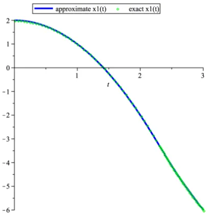
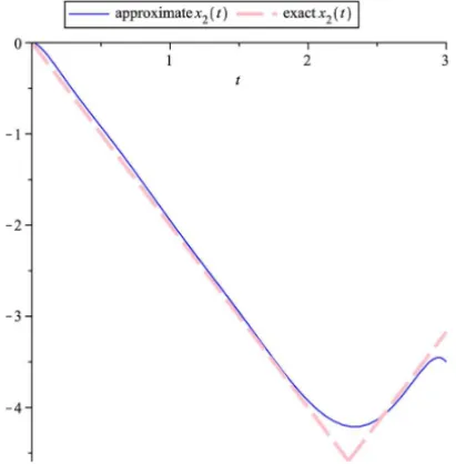
The graphs of approximated trajectoriesx1(t)andx2(t)are shown respectively
in Figure 1 and Figure 2, and the graph of approximated control is shown
Fig-ure 3. The approximated and exact objective function are respectively I =
−5.389857789,I∗= −5.528595476 (see [5]).
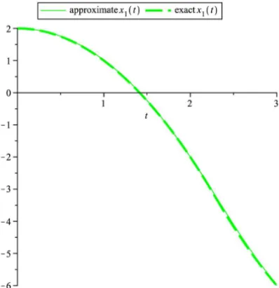
In this example, we used Bezier polynomials of degree 10 to approximate the trajectories x1(.)and x2(.) through the time interval J = [0,3], and without
using subintervals. The objective function is foundI = −5.360252730 and the
trajectoriesx1(t), andx2(t)fort ∈ J are shown in Figures 4, 5. For reduction
in complicated manipulations, the authors recommend to use low degree Bezier approximation polynomials and use subintervals approach.
Example 4.2. Consider the following optimal control problem ([17]):
min I =
Z 1 0
(x12(t)+x22(t)+0.005u2(t))dt s.t. x˙1(t)=x2(t)
˙
x2(t)= −x2(t)+u(t)
x2(t)≤q(t)=8(t−0.5)2−0.5
x1(0)=0, x2(0)= −1
Letk = 12,t0 = 0, tf = 1, tj = t0+ (tf−t0)j
12 =
j
12, (j = 1, . . . ,12), and
n=3. From (7), one can find the following solution
u(t)=
11.43511691−76.63782944t−44.52584083t2+0.0035860000t3 0≤t≤121,
7.861400876−35.62214319t−22.10043759t2+0.021243000t3 121 ≤t≤16,
8.180459190−37.33660935t−23.29089144t2−0.031848700t3 16≤t≤14,
−1.652748711−3.681790087t−.5992407498t2+0.049746000t3 14≤t≤13,
−6.522781102+8.110829441t+7.889653090t2−0.059637000t3 13≤t≤125,
−6.503100780+8.011432661t+7.992145038t2−0.00515290t3 125 ≤t≤12,
−6.497644189+7.992176154t+8.004580588t2+0.003349300t3 12≤t≤127,
−6.493920361+7.982943896t+8.007520923t2+0.00668000t3 127 ≤t≤23,
3.602879581+0.4707623628t−3.420687999t2−0.02529800t3 23≤t≤34,
11.39254692−3.778190612t−11.63683471t2+0.0188618000t3 34≤t≤56,
.9495509436−0.1355315210t−.9484970841t2−0.0070753900t3 56≤t≤1112,
Figure 1 – The graphs of approximated and exact trajectoriesx1(t)for Example 4.1.
Figure 3 – The graph of approximated control for Example 4.1.
Figure 5 – The graphs of approximated and exact trajectoriesx2(t)for Example 4.1.
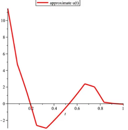
The graphs of approximated trajectories x1(t) and x2(t) are shown
respec-tively in Figure 6 and Figure 7, and the graph of approximated control is shown
Figure 8. The approximated and exact objective function respectively are I =
0.1728904530,I∗=0.17078488 (see [17]). The computation takes 5 seconds of CPU time when it is performed using Maple 12 on an AMD Athelon X4 PC with 2 GB of RAM. The QPSolve command solves (7), which involves computing the minimum of a quadratic objective function possibly subject to linear constraints. The QPSolve command uses an iterative active- set method implemented in a built-in library provided by the numerical algorithms group.
5 Conclusions
Figure 6 – The graph of approximated trajectoryx1(t)for Example 4.2.
Figure 8 – The graph of approximated control for Example 4.2.
Numerical examples show that the proposed method is reliable and efficient. The control polygon gives an intermediate approximation to the appearance of the solution.
Acknowledgment. The authors like to express their sincere gratitude to
refer-ees for their very contractive advises.
REFERENCES
[1] J. Zheng, T.W. Sederberg and R.W. Johnson,Least squares methods for solving differential equations using Bezier control points. Appl. Num. Math,48(2004), 237–252.
[2] M. Razaghi and G. Elnagar,A legendre technique for solving time-varying linear quadratic optimal control problems. J. Franklin Institute,330(1993), 453–463. [3] G.N. Elnagar and M. Razzaghi,A Collocation-type method for linear quadratic
[5] J. Vlassenbroeck,A Chebyshev polynomial method for optimal control with state constraints. Automatica,24(1988), 499–504.
[6] M. Razaghi and S. Yousefi, Legendre wavelets method for constrained optimal control problems. Mathematics Methods in the Applied Sciences,25(2002), 529– 539.
[7] M. Gachpazan, Solving of time varying quadratic optimal control problems by using Bézier control points. Computational & Applied Mathematics,30(2) (2011), 367–379.
[8] V. Yen and M. Nagurka,Optimal control of linearly constrained linear systems via state parameterization. Optimal Control. Appl. Methods,13(1992), 155–167. [9] G. Elnagar, M. Kazemi and M. Razzaghi,The pseudospectral Legendre method for discretizing optimal control problem. IEEE Trans. Automat. Control., 40 (1965), 1793–1796.
[10] P.A. Frick and D.J. Stech, Solution of optimal control problems on a parallel machine using the Epsilon method. Optimal Control. Appl,16(1995), 1–17. [11] C.P. Neuman and A. Sen,A suboptimal control algorithm for constrained problems
using cubic splines. Automatica,9(1973), 601–613.
[12] R. Pytlak,Numerical methods for optimal control problems with state constraints. First ed, Berlin: Springer-Veriag (1999).
[13] H.R. Sirisena, Computation of optimal controls using a piecewise polynomial parameterization. IEEE Trans. Automat. Control,18(1973), 409–411.
[14] H.R. Sirisena and F.S. Chou,State parameterization approach to the solution of optimal control problems. Optimal Control. Appl. Methods,2(1981), 289–298. [15] K. Teo, C. Goh and K. Wong, A unified computational approach to optimal
control problems. First edition, London: Longman, Harlow (1981).
[16] I. Troch, F. Breitenecker and M. Graeff,Computing optimal controls for systems with state and control constraints, in: Proceedings of the IFAC Control Applica-tions of Nonlinear Programming and Optimization, (1989), 39–44.
[17] H. Jaddu, Spectral method for constrained linear-quadratic optimal control. Math. Comput. in Simulation,58(2002), 159–169.
[18] M. Evrenosoglu and S. Somali, Least squares methods for solving singularity perturbed two-points boundary value problems using Bézier control point. Appl. Math. Letters,21(10) (2008), 1029–1032.