ANALYSIS, COMPARISON AND TENDENCIES OF METHODOLOGIES TO SOLVE THE NSLP

(1)

ANALYSIS, COMPARISON AND

TENDENCIES OF METHODOLOGIES

TO SOLVE THE NSLP

R. MONTOYA-ZAMORA

Faculty of Engineering, University of Querétaro, Río Moctezuma 249, San Juan del Río, Querétaro 76800, México

J. A. ROMERO

Faculty of Engineering, University of Querétaro, Río Moctezuma 249, San Juan del Río, Querétaro 76800, México

R. GUZMAN-CRUZ

Department of Research, Polytechnic University of South Zacatecas, Álvaro Obregón 11, El Remolino, Juchipila, Zacatecas 99970, México

Abstract :

Getting information of a network for different studies is very important such as to update an Origin-Destination Matrix through sensors or when it is necessary to place weight motions for an specific study and an specific kind of vehicle so the question to solve is where do they should be located? To start working it is important to get the state of art in sensor location so in this paper it is presented a chronological analysis of different methodologies found in the literature related to find the most convenient places to locate sensors which gets information about traffic and finally some comments are presented to evaluate advantages and disadvantages of each of methodology. According to these differences and some weaknesses of mathematical models it is shown the tendency to follow for future research.

Keywords: sensor location; traffic networks; network covering problems; traffic assignment.

1. Introduction

Transportation planning has been carried out pursuing different paradigms. While for road users it seems that the main interest resides in reducing traveling time and distance, for road administrator the main interest has been to provide reliable and safe roads [30]. Optimizing techniques for transportation planning have been thus employed to fulfill such needs, representing minimizations in transport costs, travel times, and distances [26]. Transportation planning involves a set of activities (trip generation, trip attraction, trip distribution and assignment) which converges in a representation of flows within a transport network. Such flows derive from an origin-destination (OD) assignment between pre-defined zones. These assignments represent the main source for decision making involving modifications in the network. Such modifications can consist of construction of new infrastructures, the widening of the existing ones, or any topological changes made to the network. A vial reorder normally includes the reassignment of the circulation in the links (e.g. changing a link from single to double way) [4]. On the other hand, new infrastructure, such as bypasses, can be built to liberate congested areas. As an example of the bypass approach, the City of Queretaro, in Mexico, has been provided with four bypasses: North, Northeast, Southwest and Northwest [5].

Matching of the assigned traffic flows with those observed in a network, is crucial for a successful planning as it signifies that a good knowledge is available regarding the network characteristics. A reliable traffic data acquisition system is thus also crucial to assess the traffic assignment associated to a transportation model. This data acquisition can be represented by a Geographic Information System (GIS) that allows the representation and the analysis of all information with a geographic character [18].

Traffic data includes a variety of mobility information, including O-D of road users, transported cargo, time distribution along the day, and the potential tariffs.

(2)

Due to the larger study area involved, regional studies are, in general, more time consuming and costly than those performed in specific spots. Research has been thus carried out to assess the effectiveness of these two approaches, further suggesting that the regional approach is less accurate than the path approach. However, the reliability of this path approach is highly dependent of the location of the data gathering stations.

Many approaches have been thus proposed for the optimal location of the mobility data gathering stations [12]; [17]; [29].

In this paper a review is presented on the research reported about the network Sensor Location Problem (NSLP) for gathering mobility information. This research aims at identifying needs for developing more realistic approaches that take into account different aspects of the traffic, such as traffic congestion. A discussion is also presented about the scope of the reported methodologies regarding its application to real complex networks, involving hundreds of centroids and average traffics of thousands of vehicles per day. It is further suggested a conceptual methodology to realize as many important traffic aspects as possible under realistic traffic environment.

2. Methodologies of NSLP

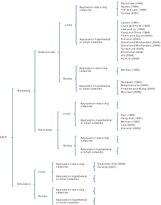
Most of the models found in the literature use deterministic procedures to solve the Network Sensor Location Problem (NSLP) and most of them place sensors on arcs instead of nodes and the majority were applied on hypothetical or small networks. Moreover non stochastic models used nodes to locate sensors and they were not proved on real or big networks and finally only two authors used simulation as a tool to solve the NSLP placing sensors on arcs and tested in real or big networks. In the following paragraphs there is a description using the kind of method used, where sensors are placed, where they were applied and listed chronologically.

2.1.Deterministic models

The following authors place sensors on links and show applications on real or big networks such as [6]. His formulation tries to catch the variables which maximize the flow information on links and then another equation finds the variables which minimize the number of sensors according to the number of information to obtain. Two heuristics were developed the first is a greedy heuristic and the second, called Ignizio’s heuristic, has a better performance but it requires more computation time than the first one because this also evaluates the information caught, and the total of information, that could be obtained if that selected link is removed. This methodology was applied to a medium size network with 114 centroids [27].

In the same year another concept of the problem was used and applied in Canada [28]. This author named the problem as the selection of count post links. Spiess used an equilibrium assignment where a set of non-decreasing link cost functions on all the links in the network ensures the convexity of the model. This methodology was applicable to big networks in the order of 1200 links and more than 500 centroids in networks such as: Swiss, Sweden and Findland.

In 1998 [35] based their methodology on [21] methodology and taking into account the link choice proportion and the available volume of traffic on links they wrote these rules with the purpose of eliminate redundant information:

(1) Rule 1: Maximal Net O-D Captured Rule: within a particular road network and for the same number of counting sensors, the best set of count locations is the one that captures the largest number of the net O-D trips and is expected to give more information for O-D estimation than others.

(2) Rule 2: Maximal Total O-D Captured Rule: when more than one set of count spots meet with the requirements of Rule 1, the best set is the batch with the largest number of total O-D trips captured at individual locations.

The procedure said that the link with the highest net OD flow will be chosen as a sensor (in each iteration) until there are not available links to be checked. If two or more links catch the same quantity of net OD flow, the one to be selected must be each one with the greatest total OD flow, always it has more independent information. They developed a heuristic algorithm.

According to them real life projects are much more massive than theoretical and formulation of objectives and determination of best surveys location are impractical. For instance in the whole Hong Kong territory are approximately 274 zones and more than 3.000 links so the linear programming approach will generate more than 225.000.000 variables and enormous computing efforts would be required. To give a solution, they propose a heuristic algorithm named Maximal O-D selection Method (MOD) as an alternative approach that identify the best group of sensors by selecting additional links one by one based on the two basic rules.

(3)

turning movements to be measured in addition to some independent total volumes at exits, entries and cross-sections inside the roundabout. After that, Tomás applied that model on a real transportation network.

Following with the chosen criteria, the next papers describe a preference placing sensors on links too but their methodologies were tested on hypothetical or smalls networks. One of the first models found in literature that follows these criteria was developed in 1981 by [20] who developed a model that was able to identify the location in which the maximum traffic flow of users occurred.

[21] developed a methodology of covering OD pairs to place sensors while [19] proposed some heuristics to define where sensors should be placed on links in a network to get a better estimation of an OD matrix.

After that [34] proposed four rules, developed a heuristic and an integer linear programming model to find sensor locations. These four rules are:

(1) OD Covering Rule: Some fraction of the OD pair must be covered by at least on sensor.

(2) Maximal flow fraction rule: For a given OD pair, the sensors should be located on the links with the largest fraction of flow for that OD pair.

(3) Maximal flow-intercepting rule: given a set of links to (potentially) monitor, choose the ones that have the greatest number of OD pairs traversing them.

(4) Link independence rule: monitor links whose flows are not dependent on each other.

Based on these rules, those links to be chosen as a sensor will be those who are independent from others, those that can intercept the maximum flow and those that can measure a bigger portion of trips for any OD pair. Using this rules, they formulated the following methods:

(1) A LP model to maximize the net traffic flows intercepted while keeping all OD pairs covered, and

(2) An application of Berman’s model [2] to formulate the entire problem as an average-reward Markov Decision Process with the objective of maximizing the net captured flows.

[29] established three factors to get the number and location of sensors: (1) The proportion ratio of the trips (OD pairs) that pass on each link. (2) The independence and inconsistency conditions of traffic flows (3) The physical conditions of links

To prioritize links, it is marked those which are used by many OD pairs and at the same time serve a large proportion of OD flows. More over the side friction factor of links and the degree of saturation are taken into account.

Finally the estimated matrix is compared to the actual one to measure the level of accuracy and in combination with the number of selected traffic counts are analyzed to find the best number and location of sensors.

[17] developed a model called “link-based model” which is a combination of three algorithms: (1) Greedy Adding (GA)

(2) Greedy Adding and Substitution (GAS) and (3) Branch and Bound (BB)

The link-based model find the set of links which get the maximum covering of OD pairs with the minimum cost of traffic counting. The main rule was adopted the links that serve a large number of OD pairs.

[11] applied an analysis to find the adequate number of image sensors on intersections to collect the necessary flows on arcs and the rate of turns to add new restrictions to estimate, with a unique solution, OD pairs.

[12] created a new set of network location problem which determine where to locate active sensors to obtain the maximum information on flow volumes on specified paths. There are distinguished 3 different scenarios: zero count information, total count information and partial count information. They use the rank of a link-path incidence matrix to verify if a system of linear equations is determinable, and to determine the number and locations of active sensors on specific links in order to provide additional path flow information to infer the complete flow estimates on all paths. Hogberg pointed that links with high expected flows and links that pass through OD pairs and that have to be counted on other links are more valuable than others [10].

[13] define the concept of and edge control set. This is a set of edges S in a graph such that if two network flow functions are given, then the functions are equal everywhere. In other words if the flow on every edge in S is known, the flow everywhere in the graph can be determined by simply finding a flow function on the graph that matches the values determined on S. This algorithm can be solved when the graph follows two conditions: first all links in the graph lie on some directed cycle and second there are no sources or sinks in the graph.

[7] based their work on Yang and Zhou’s and developed a software tool based on Mixed Integer Programming techniques which solves the complex problem formulated only mathematically by Yang and Zhou. This software includes the extension of Chung’s budget constraint and a set of weight for ranking OD pairs by importance. These two new elements includes are:

(4)

(2) Weighting rules: some OD pairs are more important and more interesting than others for the manager in other words some links are more informative than others.

[32] developed a model based on [33]. In Yang’s model no information is needed for the travel times on the network and it does not use the network capacity as a parameter but in this model the statistical concept of the Maximum Possible Relative Error (MPRE).

They used link travel times in the objective function so they took into account capacities. It is considered that by adopting a dynamic network loading model for computing the travel times on all links it can account for the temporal variation of flows more correctly, the objective explicitly accounts for the relationship between flows and travel times among links.

In this model it is reformulated the MPRE, originally proposed to compare OD flows, for measuring the deviation between real and estimated link travel times it can be obtained more detailed information than the classical NSLP taking travel times from GPS data and assuming that route travel times are in equilibrium. The modified algorithm follows these steps:

(1) Solve the OD coverage algorithm and find the minimum number of sensors needed to cover all ODs. (2) Find the sensor among the OD Coverage solution that has the largest correlation with other links and

remove monitored link flow correlations from the correlation matrix.

(3) Recompute the OD coverage algorithm and find the new most representative link to be monitored.

(4) Stop when a maximum value of sensors has been placed or a minimum percentage of flows has been caught.

[16] change the paradigm using the concept of basis links to solve the network sensor location problem. To solve this problem they first create an incidence matrix formed by all the paths in the network placed as rows and the links on the network placed as columns. This matrix is filled with 1 when the link is part of a path and 0 when it is not. In this paper this matrix space is also considered as a vector space so it has a rank. To solve the problem the concept of reduced row echelon form is introduced to identify the basis links of the link-path incidence matrix.

They establish that any column vector can be represented by a linear combination of a set of r unit column vectors whose linear combination coefficients α are the column elements corresponding to the nonzero rows. The information of this basis links are used to completely describe the network structure. On those basis links sensors are placed

The Model which place sensors on nodes and were applied on a real network was developed in 1992 by [2] and it returned to the idea of using the maximum number of customer flows and this model was based on Hakimi’s and Hogson’s model. This new model makes the assumption that a person travels (as a one stop tour) from his home to the service facility, consumes the service and returns home. Berman’s model makes these assumptions: (1) Customer’s flows along all paths of the transportation network are known.

(2) Only the flow that passes through a facility is considered as intercepted.

(3) The service facilities have sufficient capacity so that no waiting lines in front of the facilities exist

In other words the customer does not embark only in one stop in contrast the customer has a preplanned trip and passes by more than one discretionary service facilities on his route. In this model it is assumed that planners know travels between OD pairs and they can get flow rates to locate a determined number of discretionary service facilities on the network that maximize the flow of potential customers that pass at least by one of the service facilities.

The problem was formulated as an integer linear problem and solved using a greedy heuristic to locate facilities sequentially at nodes which intercept most of the non intercepted flow. The heuristic was coded in PASCAL and tested for networks with nodes and paths ranging from 10 to 100 and they proved that in 65% the heuristic produced the optimal solution.

Those models placed on nodes and that were tested on hypothetical networks are described in the following paragraphs.

There is a register of other models that were reported in literature until 1990. The first of them is developed by [15] who used the Flow Covering Location Allocation Model (FCLM). The FCLM is considerer a special case of the maximal covering location problem and it uses the maximum flow to maximize information. To solve this problem there were used two heuristics:

(1) Multiple Coverage Greedy Heuristic chooses the p nodes, with the greatest flows, passing through them. Flows that pass through a node and were selected in one step may be counted again in a subsequent step. (2) Non-Multiple Coverage Greedy Heuristic chooses the p nodes, with the greatest flows, passing through

them but when a node is selected all flows that pass through a node are removed.

Even when this methodology gets the best solution for O-D pairs and flows, it finds the shortest paths between each origin-destination pair that could be equivalent to use an All or Nothing Assignment.

(5)

Matschke and Friedrich have been concluded that could be a better estimation of and OD matrix with link information of flows and turning flows [23].

Friedrich and Wang [10] applied four indices to prioritize counting intersections according to their contribution to OD matrix. He concluded that according with the results turning flows contribute with more information than inbound link flows at intersections.

Morrison [25] places sensors at intersections (vertices) and uses an undirected graph. Here it is established the flow conservation at each vertex and those vertex with non-zero balancing flows are called bound vertex.

2.2.Stochastic models

The following authors used stochastic models to solve the NSLP and place sensors on links and show applications only on small networks such as Han in 1983 that used a strategy to get information through traffic counts in a network where he included two factors: location (where sensors are placed) and covering (the percentage of counted links). Due to location three strategies were considered: random selection method, major locations and geographic patterns. A model named LINKOD was developed that works for small and congested areas.

Yang et al [33] proposed the so-called OD covering rule to locate sensors on arcs to bound the OD estimation error. After that In 1995 Berman et al followed the same rules established before but this time they assigned flows in a probabilistic manner to know customer’s travel decisions that are not reflected in a deterministic model such as All or Nothing [2].

They formulate the problem as an average-reward Markov Decision Process (MDP) and the objective functions was focused on finding a set of locations for the m facilities that maximize the total flow intercepted excluding double counting. To solve the problem, they established two formulations from integer variables. To make this simpler they formulate an equivalent nonlinear formulation of the problem and they demonstrated its equivalent to the first formulation.

Finally they created a greedy heuristic to locate facilities sequentially at nodes which intercept most of the unintercepted flow that still remains in the network. As it can be seen, this is a similar procedure followed by Hodgson [15] and De la Llata [6].

In 2002, Lotz proposed a rule taking into account the precision of the OD pairs estimated (getting the average deviation between the estimated and the sized OD flows for each OD pair) [22]. According to this, the link which contributes with less deviation will be chosen as a sensor.

Kim et al. [17] using the model called “link-based model” described before used also an stochastic procedure to solve the NSLP.

2.3.Simulation

Only two authors present a solution to solve the NSLP using simulation and of course taking into account time variations these authors are:

Eisenman et al [8] view the NSLP from a perspective of value of information. Here it is mentioned that sensors continuously provide information that helps characterize the status of a network and using this information in conjunction with knowledge could enhance a model’s estimation and prediction performance. They used the software Dynasmart-X to simulate using historical information and real time information. The model is a continuous learning model that receives real time information and uses an iterative process to incorporate this information and improve the quality of estimation and prediction.

Moreover the NSLP is viewed as traffic status learning process that needs more sensors to add valuable information that can be used to update estimates of the network traffic status.

This methodology was applied in Maryland Chart network with 2,182 nodes, 3,387 links and 111 zones.

Fei et al [9] proposed a new solution for the OD covering problem with time-varying flows obtained by simulation with Dynasmart. Then they used Kalman filtering techniques to correlate the information content of each sensor position and thus minimize the error in the OD matrix estimation. According to this methodology authors included dynamic and stochastic characteristics by means of simulation.

(6)

Conclusions

In agreement with Hu network topology is a determinant key of the number of sensors to be installed. This paper takes into account topology of network while others evaluate sensor location by flows on links.

Yang and Zhou’s rules are proposed according to the experience but not mathematically. The first and the fourth rules are satisfied always in any distributions of sensors but the other two rules are much more difficult to satisfy because they often come into conflict with the other rules so rules two and three cannot both always be completely satisfied.

Yang’s method assumes that link counts are error free which means that would be always an error in location of sensors if traffic and time variation is taken into account.

Most of these methods are static they do not take into account time variation. Most of these techniques are applied on networks with few links and centroids.

Most of these methodologies solve the problem using heuristics instead of using linear programming.

Most of these methodologies do not take into account some externalities such as road pricing and environmental N S L P

M o d e l li n g

D e te r m i n i stic

L i n k s

N o d e s

A p p l i e d o n r e a l o r b i g n e tw o r ks

A p p l y e d o n h yp o th e tic al o r s m a l l n e tw o rk s

L a r s o n ( 1 9 8 1 )

A p p l y e d o n r e a l o r b i g n e tw o r ks

H o d g so n ( 1 9 9 0 ) D e l a L l a ta ( 1 9 9 0 ) S p i e s s ( 1 9 9 0 )

L o g i e a n d H y n d ( 1 9 9 0 ) L a m a n d L o ( 1 9 9 0 )

B e r m a n ( 1 9 9 2 ) Y i m a n d L a m ( 1 9 9 8 )

Y a n g a n d Z h o u ( 1 9 9 8 ) T o m á s ( 2 0 0 1 )

T a m i n a n d S u y u ti ( 2 0 0 3 ) K i m e t a l ( 2 0 0 3 )

M a ts c h k e e t a l ( 2 0 0 4 ) G e n ti l i a n d M i r ch a n d a n i ( 2 0 0 4 )

F r i e d r ich a n d W a n g ( 2 0 0 5 ) G e n ti l i a n d M i r ch a n d a n i ( 2 0 0 5 ) G u a n d J i a ( 2 0 0 5 )

E l h e r t e t a l ( 2 0 0 6 ) V i ti ( 2 0 0 8 )

M o r r i so n ( 2 0 0 8 ) H u e t a l ( 2 0 0 9 )

S to c h a s tic

L i n k s

N o d e s

H a n ( 1 9 8 3 ) A p p l y e d o n r e a l o r b i g

n e tw o r ks

Y a n g e t a l ( 1 9 9 1 ) B e r m a n ( 1 9 9 5 ) L o tz ( 2 0 0 2 ) K i m e t a l ( 2 0 0 3 )

S i m u l a ti o n L i n k s

N o d e s

E i s e n m a n e t a l ( 2 0 0 6 ) F e i e t a l ( 2 0 0 7 )

(7)

Methodologies presented do not evaluate road characteristics such as: altitude, curvature, fuel consumption; or drive style, acceleration, aggressive style of driving, desired speed.

No methodology uses another technique to solve the NSLP such as Genetic Algorithms (GA) because this technique finds a global, not local, solution as linear, integer or non linear programming.

No methodology takes into account pavement conditions and the style of driving as variables for selecting routes and route time.

This paper has included and discussed issues associated with optimizing detector locations for OD matrix estimation, and proposed some important factors that can effectively take into account the budget constraints and the OD coverage.

The purpose of giving these recommendations is to have a better understanding of which of this can be taken into account when a sensor should be placed into a real network.

A future research will be focused on establish a relationship between the characteristics of links and location of sensors taking into account the interception rule and the maximal flow fraction on various types of networks. Moreover future researchers should take into account subsets of networks, global solutions and a different focus for getting information from networks for example location of weight motions for a specific kind of vehicles on a specific kind of roads and for some specific conditions of pavements.

Few of the methodologies use a Geographic Information System and its applications to analyze the NSLP with a different point of view such as topology or accessibility.

References

[1] Beasley, J. E.; Chu, P. C. (1996): A genetic algorithm for the set covering problem. European Journal of Operational Research, 94, pp. 392-404.

[2] Berman O, Krass D, Xu CW (1995): Locating discretionary service facilities based on probabilistic customer. Transportation Science. 29, pp. 276-290.

[3] Berman O, Larson RC, Fouska N (1992): Optimal location of discretionary service facilities. Transportation Science. 26, pp. 201-211. [4] Chin SM, Hwang HL (2006): Converting Freight Flow information to Truck Volumes. Transportation Research Board 2006 Annual

Meeting, Washington, D.C.

[5] CONCYTEQ (2001): Transportation diagnosis. Queretaro Council for Science and Technology. (In Spanish) ISBN 968-5402- 03-5. Querétaro. p. 120.

[6] De la Llata R (1990): Estrategias para la realización de Estudios Origen-Destino. Instituto Mexicano del Transporte. Publicación Técnica 48.

[7] Ehlert A, Bell MGH and Grosso S. (2006): The Optimisation of traffic count locations in road networks. Transportation Research Part B. 40B, pp. 460-479.

[8] Eisenman SM, Fei X, Zhou X. and Mahmassani HS. (2006): Number and Location of Sensors for Real-Time Network Traffic Estimation and Prediction. Sensitivity Analysis. Transportation Research Record, 1964, pp. 253-259.

[9] Fei X, Mahmassani HS and Eisenman SM. (2007): Sensor coverage and Location for Real-Time Traffic Prediction in Large-Scale Networks. In Transportation Research Record: Journal of the Transportation Research Board, No. 2039, Transportation Research Board of the National Academies, Washingtong, D.C., pp 1-15.

[10] Friedrich B, Wang YP (2005): Effectiveness of data composition on OD matrix estimation. Institute of Transport, Road Engineering and Planning. University of Hannover. Hannover, Germany.

[11] Gentili M, Mirchandani P (2004): Locating Image Sensors on Traffic Networks. Proceedings of the Triennial Symposium on Transportation Analysis TRISTAN V. Le Gosier, Guadeloupe, French West Indies.

[12] Gentili M, Mirchandani P (2005): Locating Active Sensors on Traffic Networks. Annals of Operations Research. 136, pp. 229-257. [13] Gu W, Jia X (2005): On a traffic Control Problem. Proceedings of the 8th International Symposium on Parallel Architectures,

Algorithms and Networks.

[14] Han AF, Sullivan EC (1983): Trip table synthesis for CBD networks: Evaluation of the LINKOD model. Transportation Research Record 944, TRB, National Research Council, Washington, D.C. pp. 106-112.

[15] Hodgson MJ (1990): A flow-capturing location-allocation model. Geographical Analysis, Annals of Operations Research. 22, pp. 271-279.

[16] Hu SR, Peeta S, Chu CH (2009): Identification of Vehicle sensor locations for link-based network traffic applications. Transportation Research Part B. 43, pp. 873-894.

[17] Kim HJ, Chung IH, Chung SY (2003): Selection of the Optimal Traffic Counting Locations for Estimating Origin-Destination Trip Matrix. Journal of the Eastern Asia Society for Transportation Studies. 5, pp. 1353-1365.

[18] Lakhoua MN (2010): Information analysis and geographic information system (GIS) exploitation in a grain silo. Journal of Engineering and Technology Research. 2(10), pp. 195-199.

[19] Lam WHK, Lo HP (1990): Accuracy of OD estimates from traffic counts. Traffic Engineering and Control. 31, pp. 358-367. [20] Larson R, Odoni B (1981): Urban Operations Research. Prentice-Hall.

[21] Logie M, Hynd A (1990): MVESTM matrix estimation. Traffic Engineering and Control. 31, pp. 454-459.

(8)

[23] Matschke I, Friedrich B (2001): Dynamic OD Estimation Using Additional Information from Traffic Signal Lights Timing. Proceedings of the Triennial Symposium on Transportation Analysis TRISTAN IV. Sao Miguel - Azores, Portugal. pp. 589-593. [24] Matschke I, Friedrich B, Heinig K (2004): Data Fusion Technique in the Context of Traffic State Estimation. Proceedings of the

Triennial Symposium on Transportation Analysis TRISTAN V. Le Gosier, Guadeloupe, French West Indies.

[25] Morrison DR, Martosoni S, Tucker K (2008): Characteristics of Optimal Solutions to the Sensor Location Problem. Thesis. Harvey Mudd College, Department of Mathematics.

[26] Ng WS, Schipper L (2006): China Motorization Trends, Consequences and Alternatives. Transportation Research Board Annual Meeting. Washington, D.C.

[27] Secretaría de Comunicaciones y Transportes (1988): Sogelerg, Programación Sectorial del Transporte, Esquemas Directores Subsectoriales, Subsector Carretero, Anexos Técnicos. México. pp. 935-964.

[28] Spiess H (1990): Conical Volume-Delay Functions. Transportation Science. 24(2), pp. 153-158.

[29] Tamin OZ, Suyuti R (2003): The Impact of Location and Number of Traffic Counts in the Accuracy of O-D Matrices Estimated from Traffic Counts under Equilibrium Condition: A Case Study in Bandung (Indonesia). Journal of the Eastern Asia Society for Transportation Studies. 5, pp. 393-1407.

[30] Taniguchi E, Imanishi Y (2008): Methodology and effects of heavy goods vehicle transport management in urban areas. 10th Heavy Truck Conference. Paris, France.

[31] Tomás AP (2001): Modelling Optimal Location of Traffic Counting Points at Urban Intersections in CLP (FD). Technical Report Series DCC-2001-4. Departamento de Ciência de Computadores – Faculdade de Ciências & Laboratorio de Inteligencia Artificial e Ciência de Computadores Universidade do Porto, Portugal.

[32] Viti F, Verbeke W and Tampère ChMJ. (2008): Sensor Locations for Reliable Travel Time Prediction and Dynamic Management of Traffic Networks. Transportation Research Record: Journal of the Transportation Research Board 2049, pp. 103-110.

[33] Yang H, Iida Y, Sasaki T (1991): An Analysis of the Reliability of Origin-Destination Trip Matrix Estimated from Traffic Counts. Transportation Research Part B. 25(5), pp. 351-363.

[34] Yang H, Zhou J (1998): Optimal traffic counting locations for origin-destination matrix estimation. Transportation Research Part B. 32, pp. 109-126.