A Patch-by-Patch Shape Matching Procedure for
Rigid Body Docking
Vipin K. Tripathi
∗Abstract—Docking simulates molecular interac-tions. Protein - protein docking, owing to the sizes of molecules, is a very challenging problem. As the num-ber of degrees of freedom in the molecular structure of proteins is huge, docking algorithms consider the molecules as relatively rigid bodies. Shape matching of two protein molecules is computationally difficult because the possibilities of matching the molecules grow exponentially with the size of molecules which gives a large search space. A new scheme is proposed in this paper for shape matching in rigid body dock-ing. The scheme models the molecular surface as a network of locally characterized surface patches con-nected to each other at their boundaries. For shape matching of molecules, a patch-by-patch shape match-ing strategy is used. The procedure suggested for shape matching can be easily included in an optimiza-tion routine for finding the best binding conforma-tions of two protein molecules.
Keywords: docking, shape matching, bioinformatics, computer aided design
1
Introduction
Computational molecular docking aims at finding the best binding conformations of two given molecules. The molecules may be two protein molecules or a protein and a ligand molecule. Docking is important in relation to molecular recognition, macromolecular assemblies, cellu-lar pathways, protein folding etc. [1]. It has an indus-trial application in rational drug design [2]. A compre-hensive review of the docking algorithms can be found in [3]. Docking of two molecules is shown in Figure 1. The patches on the surface of outer molecule are indi-cated by small triangles. Lines indicate the boundaries of the patches.
A computational docking procedure involves three steps: (i) shape representation of molecules (ii) shape match-ing and (iii) optimization of shape matchmatch-ing. Generally, the methods used for docking are, broadly, classified into two categories: rigid body docking and flexible ligand
∗Mechanical Engineering Department, Government Engineer-ing College Aurangabad, Maharashtra India 431005. Email: vipinkt [email protected]. Author is thankful to Santosh Tiwari, Research Associate at I.I.T. Kanpur, for helping in elegant imple-mentation of the algorithm proposed in this paper. Manuscript submitted on 13th March, 2007
Figure 1: Docking of two molecules
docking. The rigid body docking methods consider both the molecules as rigid bodies, whereas the flexible ligand methods consider one or both the molecules flexible.
Different mathematical model have been used for molec-ular shape representation. Connolly [4] laid the founda-tion of representing the molecular surface by its geometric features. Lin et al. [5] describe the surface by sparse crit-ical points. Sanner et al. [6] compute a reduced surface in their MSMS algorithm. Some researchers have used ‘shape-implicit’ methods which discretize the molecule onto a grid in space and consider only the occupied cells, i.e., voxels, to define the shape of the molecule [7].
The shape matching procedure proposed in this paper, considers molecular surface as a network of locally char-acterized surface patches connected to each other at their boundaries. Those surface patches of the molecules are modeled by B-spline surface representation technique. In the process, an inverse problem in the B-spline surface fitting is solved. B-spline surface approximation tech-nique offers a lot of flexibility required for fitting a surface through scattered data [8]. It is, therefore, a promising shape representation technique for molecular docking. A number of studies [9] focus on modeling a surface patch from 2-D parameterized data points. The procedure used in this study for modeling the surface patches is described in section 2 of this paper.
problem. Many approaches have been tried for shape matching in docking. These matching algorithms may be classified into two broad categories: (i) brute force enu-meration algorithms and (ii) local shape feature match-ing algorithms. Local shape feature matchmatch-ing algorithms have been pioneered by Kuntz [10]. These algorithms use complementary features of surfaces to align them. They include algorithms like distance geometry algo-rithms [10], pose clustering [7], geometric hashing and geometric hashing and pose clustering.
In the present study, a different approach is proposed for shape matching of the molecules. A point on each of the two surfaces and a triad of three mutually perpen-dicular unit vectors at each of the two points is used as local shape feature for matching the surface patches from two different molecules. An association of two molecules can be rated as correct or incorrect based on different criteria like shape complementarity between molecules, binding energy of a complex, electrostatic and van der Waals interactions etc. Although other criteria are also important, shape complementarity is considered a neces-sary condition in rigid body docking. Shape complemen-tarity criterion was initially adopted by Kuntz and his colleagues [10] and was further elaborated and rational-ized by Connolly [11]. Here also, shape complementarity has been used as the criterion for matching of the sur-face patches. For shape matching, only the patches with complementary curvatures are aligned with each other. The method proposed here is simple and effective. It can easily be used in an optimization routine with a suitable scoring function to find the best binding conformations.
2
Modeling of Molecular surface
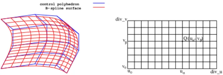
The molecular surface is considered to be made up of sur-face patches of different forms such as convex, concave , flat etc. connected to each other. B-spline surface rep-resentation technique is used in this paper to generate the patches of molecular surface. The B-spline surface is controlled by a characteristic polyhedron as shown in Figure 2. Advantages of this surface are the local control of surface and independence of the degree of surface from number of control points. The surface generation scheme requires molecular data already parameterized on a 2-D grid as input. The rectangular data grid is shown in Fig-ure 3.
A tensor product B-spline surface is formulated as
Q(u, v) =
n
X
i=0
m
X
j=0
PijNi,k(u)Nj,l(v) (1)
control polyhedron B− spline surface
Figure 2: B-spline surface
uα
β Q
div_v
div_u ( uα,vβ)
u
0
v
0
v
Figure 3: Rectangular 2-D grid of data points
where
Q(u, v) = a point on the surface,
Pij = vertices of the defining
polyhedron,
Ni,k(u), Nj,l(v) = blending functions in u,
v directions, respectively.
k, l = orders of curves in u, v directions, respectively.
The B-spline blending functions are computed by the fol-lowing recursive expressions:
Ni,1(u) =
1 ifti ≤u < ti+1,
0 otherwise. (2)
Ni,k(u) =
(u−ti)Ni,k−1(u)
ti+k−1−ti
+(ti+k−u)Ni+1,k−1(u)
ti+k−ti+1
(3)
Theti are known as knot values. They relate the
para-metric variable u to the control pointsPij. For an open
curve,ti are given by
ti=
0 ifi < k,
i−k+ 1 ifk≤i≤n,
n−k+ 2 ifi > n,
(4)
with
0≤i≤n+k. (5)
The range of parametric variableuis
0≤u≤n−k+ 2. (6)
Finding Q, the surface data points, by an input of (n+ 1)×(m+ 1) number of control points which are the vertices of control polyhedron Pij, is known as the
‘forward problem’.
the method used here for solving the inverse problem are given below.
Writing out Eq. 1 for a single surface data point, say, pointQ(uα, vβ) as shown in Figure 3 yields
Q(uα, vβ) =
N0,k(uα) · · · Nn,k(uα) Pij
N0,l(vβ)
N1,l(vβ)
.. .
Nm,l(vβ)
. (7)
Writing an equation of this form for each data point on the rectangular grid yields a system of simultaneous equa-tions. In the matrix form the result can be written as
[Q] = [Ct][Pij][D] (8)
whereQis the matrix of data points. It has (div u+ 1)× (div v+1) elements in it. CTis the matrix of row vectors
on the right hand side of Eq. 7. It contains (div u+ 1)× (n+ 1) elements. P is a matrix of control points. It contains (n+ 1)×(m+ 1) elements. D is the matrix of column vectors on the right hand side of Eq. 7. It contains (m+ 1)×(div v+ 1) elements.
Eq. 8 is simplified to the standard form,
q= [A]p (9)
where
q =Column vector of data points of dimension (div−u+1)*(div−v+1),1,
p =Column vector of control points of dimension (n+1)*(m+1),1,
[A] =Matrix of dimension
(div−u+1)*(div−v+1),(n+1)*(m+1).
Matrix [A] is formed as,
AI,J =dJ,I[Ct] (10)
where d(J,I) =(J, I)thelement of D matrix.
As the surface point data available in molecular dock-ing problem will give a highly over-specified matrix A, system [ATA]p= [AT]q is solved instead of the system Ap=q, using Cholesky decomposition of matrixA[12]. Matrix [ATA] on the left hand side is a square ma-trix then. If Cholesky decomposition fails due to mama-trix
[ATA] not being positive definite, a method based on singular value decomposition is used which is applicable to a general rectangularM×N matrix. For detailed dis-cussion related to the procedure used for modeling the molecular surface [13] can be referred.
3
Molecular Shape Matching
A patch by patch matching strategy is used for shape matching of the two molecules. After solving the inverse problem, the control points of the two surface patches, one from each of the two molecules, are available. The problem of surface matching can now be described as:
1. Given the control points of two surface patches, check whether the patches are complementary.
2. If the patches are complementary, (i) compute the translation required to match two given surface patches at a point and (ii) compute the rotation required to match the surface patches in the same orientation.
Before matching the surface patches of two different molecules, they are checked for complemetarity as de-scribed in the following section.
3.1
Check
for
Complementary
Surface
patches
To check if the surface patches are complementary, the principal curvatures of both the surface patches are cal-culated by Eq. 11.
κmax=H+
√
H2−K κmin=H−
√
H2−K. (11)
In Eq. 11, H is mean curvature and K is Gaussian curva-ture [8].
If
κmax1 = maximum curvature of the first surface
patch at the matching point,
κmin1 = minimum curvature the first surface
patch at the matching point,
κmax2 = maximum curvature of the second
surface patch at the matching point,
κmin2 = minimum curvature the second surface
patch at the matching point,
the surface patches arenotcomplementary whenκmax1× κmax2>0 orκmin1×κmin2>0.
3.2
Computing the Translation and
Rota-tion for the Surface Patches
3.2.1 Translation
For matching the surface patches at a given point on both the surface patches, the strategy used here is to translate both the surface patches to the origin of the coordinate frame such that the given matching points on both the surface patches coincide with the origin.
The translation for the first surface patch is computed by the following equation
P1ijT =P1ij−Q1 (12)
where
P1ij = control points of the first
surface patch,
−Q1 = translation for the first surface patch,
P1ijT = changed control points of
the first surface patch after translation .
New control points will generate the surface patch in translated position, i.e., at the origin. This is due to the property of B-spline basis functions known as ‘partition of unity’.
Translation for the second surface Patch is computed by
P2ijT =P2ij−Q2 (13)
where
P2ij = control points of the second
surface patch,
−Q2 = translation for the second surface patch,
P2ijT = changed control points of
the second surface patch after translation.
Changed control points will generate the second surface patch in translated position such that the given match-ing point on the second surface patch will coincide with the origin and thus, with the matching point on the first surface patch. This completes the translation of surface patches.
3.2.2 Rotation
Translation brings the surface patches at the origin where they meet each other at a point. But it does not change their orientation. The next task is to find the required rotation which will re-orient and superimpose one surface patch over the other. This is required to judge as to how well they match with each other.
The strategy used to match the surface patches in the same orientation is to compute a triad of unit vectors at the given point on both the surface patches and then to match these unit vectors of a triad with the coordinate axes. A triad at the matching point on any of the two surface patches consists of three unit vectors: a unit tan-gent vector in u parametric directionqu, a unit normal
to the surface patch n and a unit vector m normal to both of qu and n (refer [8]). A matrix V is formed by
writing vectors of a triad in the rows of the matrix and a matrix W is formed similarly by the coordinate axes vectors. SinceVandWare unit vector matrices, it can be written
[x y z]T = [q
u1 m1 n1]T[R].
Then, required rotation matrix for systemVwith respect to systemWis simply
[R] = [V]−1[W]. (14)
Using Eq. 14 now, changed control points of the surface patches after rotation can be obtained. For the first sur-face patch,
P1ijR=P1ijT ×R1 (15)
where
R1 = rotation matrix for the first
surface patch,
P1ijR = changed control points of the
first surface patch after rotation.
Similarly, for the second surface patch,
P2ijR=P2ijT ×R2 (16)
where
R2 = rotation matrix for the second
surface patch,
P2ijR = changed control points of the
second surface patch after rotation.
Changed control points will generate the surface patches in rotated position. If both the surface patches are gener-ated with the changed control points and plotted on the same plot, they match in the same orientation.
4
Proposed Algorithm
Algorithm proposed for matching two surface patches at a point and in same orientation is as follows:
Step 2 : Compute the principal curvatures of both the surface patches and check for complementarity as in section 3.1.
Step 3 : If surface patches are complementary, input the values of parameters u and v for a point and the control points P1ij for the first surface patch. Find
translationQ1by Eq. 1.
Step 4 : Obtain changed control points of the first sur-face patch after translationP1ijT, using Eq. 12.
Step 5 : Compute triad (qu1,m1,n1) and form matrix Vas [qu1,m1,n1]T.
Step 6 : If principal curvatures of the first surface patch are positive, form matrixWas [x,y,z]T and if they
are negative, form matrixWas [x,y,−z]T.
Step 7 : Find rotation matrixR1, using Eq. 14.
Step 8 : Obtain changed control points of the first sur-face patch after rotationP1ijR, using Eq. 15.
Step 9 : Repeat steps 3 to 8 for the second surface patch.
Step 10 : Generate both the surface patches using changed control points after rotation P1ijR and
P2ijR in Eq. 1. Plot both the surface patches in
the same plot to see the match.
5
Simulation Results and Discussion
A few results of testing the algorithm given in the previ-ous section on different types of surface patches are shown here. The surface patches are generated by method given in section 2 using already available 2-D parameterized data sets. The algorithm is, yet, to be tested on actual protein data available in protein data bank. For gener-ation of surfaces, 651 data points have been used in a data set. The curves in u and v parametric directions are cubic. The algorithms are coded in C programmming language and the results are displayed ingnuplotinlinux
environment.
Two surfaces patches are shown in Figures 4 and 5 from two different molecules which are to be matched at a given point and in the same orientation. The first sur-face patch is a concave sursur-face patch while the second surface is a convex one. Figure 6 shows both the surface patches in translated position. The given points of both the surfaces coincide with the origin of the coordinate frame in the translated position. Thus, the surfaces meet each other at the origin. To show this aspect, scale is plot-ted in the figure. Both the surfaces are shown in rotaplot-ted position in Figure 7. In the rotated position both the surfaces are matching in the same orientation. Another matching of the two different patches shown in Figures 8 and 9 is displayed in Figure 10. A matching of two flat
surface patches from two different molecules is shown in Figure 11. These results demonstrate the effectiveness of the algorithm for shape matching.
Figure 4: Surface patch from the first molecule
Figure 5: Surface patch from the second molecule
−20 −10
0 10
20 −20
−10 0
10 20
−20 −10 0 10 20
Figure 6: Surface patches translated to the origin (the first step)
6
Conclusions and future work
−10
−5
0
5
10
15
20
25
−25
−20
−15
−10
−5
0
5
10
0
2
4
6
8
10
12
14
16
18
20
Figure 7: Surface patches rotated to match in the same orientation (the second step)
Figure 8: Surface patch no. 2 of the first molecule
Figure 9: Surface patch no. 2 of the second molecule
References
[1] Tsai, C. J., Xu, D., Nussinov, R., “Protein folding via binding and vice versa,” Fold Design pp. R71– R80 3/98
[2] Abagyan, R., Totrov, M., “High throughput docking for lead generation,”Curr Opin Chem Biol, pp. 375– 382, 5/01
[3] Halperin, I., Ma, B., Wolfson, H., Nussinov, R., “Principles of Docking: An Overview of Search Algo-rithms and a Guide to Scoring Functions,”Proteins, pp. 409–433, 47/02
[4] Connolly, M., “Analytical molecular surface calcula-tion,”J. of Appl. Cryst., pp. 548–558, 16/83
[5] Lin, S. L., Nussinov, R., Fischer, D., Wolfson, H. J., “Molecular surface representation by sparse critical points,”Proteins, pp. 94–101, 18/94
[6] Sanner, M. F., Olson, A. J., Spehner, J. C., “Re-duced surface: an efficient way to compute molecular surfaces,”Biopolymers, pp. 305–320, 38/96
Figure 10: Surface patch no. 2 of the first molecule matching with patch no. 2 of the second molecule
Figure 11: Two flat surface patches from different molecules matching with each other
[7] Goldman, B. B., Wipke, W. T., “QSD quadratic shape descriptors. 2. Molecular docking using quadratic shape descriptors (QSDock),” Proteins, pp. 79–94, 38/2000
[8] Mortenson, M. E.,Geometric Modeling, John Wiley and Sons (1985)
[9] Tripathi, V. K., Dasgupta, B., Deb, K., “An ap-proach for surface generation from measured data points using B-splines,” Int. Conf. on Systemics, Cybernetics and Informatics, Hyderabad, India, pp. 578–581, 2005
[10] Kuntz, I., Blaney, J., Oatley, S., Langridge, R., Fer-rin, T., “A geometric approach to macromolecule-ligand interactions,” J. of Mol. Biol., pp. 269–288, 161/82
[11] Connolly, M., “Shape complementarity at the hemoglobin α1β1 subunit interface,” Biopolymers
pp. 1229–1247, 25/86
[12] Kreyszig, E., Advanced Engineering Mathematics, 8th Edition, John wiley & sons, inc., New York, 2002