SRef-ID: 1432-0576/ag/2005-23-3229 © European Geosciences Union 2005
Annales
Geophysicae
A complex autoregressive model and application to monthly
temperature forecasts
X. Gu1and J. Jiang2
1State Key Laboratory of Sever Weather, Chinese Academy of Meteorological Sciences, Beijing, 100081, China 2Training Center of China Meteorological Administration, Beijing, 100081, China
Received: 26 June 2005 – Revised: 19 September 2005 – Accepted: 20 September 2005 – Published: 30 November 2005
Abstract. A complex autoregressive model was established based on the mathematic derivation of the least squares for the complex number domain which is referred to as the com-plex least squares. The model is different from the conven-tional way that the real number and the imaginary number are separately calculated. An application of this new model shows a better forecast than forecasts from other conven-tional statistical models, in predicting monthly temperature anomalies in July at 160 meteorological stations in mainland China. The conventional statistical models include an au-toregressive model, where the real number and the imaginary number are separately disposed, an autoregressive model in the real number domain, and a persistence-forecast model.
Keywords. Ionosphere (Modeling and forecasting) – Gen-eral (Instruments useful in three or more fields)
1 Introduction
The classical least-squares method in the real number do-main is widely employed in statistics for establishing regres-sion models (e.g. Kendall and Stuart, 1976; Montgomery and Peck, 1982; Kern et al., 1987; Kleinbaum et al., 1988), even in the mathematics-physical method for calculating spherical harmonic coefficients (e.g. Ge et al., 1980). However, few reports of the complex least-squares method and the com-plex autoregressive model were found in the atmospheric or geophysical sciences before. As is well-known, once a sta-tistical method has been extended to the complex number domain, it has gotten some new functions and gives more information. For example, the CEOF (Complex Empirical Orthogonal Function), which is an extension from the EOF (Empirical Orthogonal Function) in the real number domain Correspondence to:X. Gu
(guxq@cams.cma.gov.cn)
to the complex number domain, acquires a new function of decomposing variations of patterns and phase of the travel-ing waves on various space scales (e.g. Rasmusson et al., 1981; Barnett, 1983), while the EOF decomposes only the stationary waves in an element field in meteorology or geo-physics. It should obtain an improvement when the classical least-squares method and the autoregressive model were ex-tended to the complex number domain.
The spherical harmonic coefficient in the global spectrum model in meteorology is in the complex number. Gu (1998) derived the complex least-squares method to have resolved complex auto-memory coefficients, then established a global auto-memory spectrum model, and obtained a good forecast-ing effect for a 500-mb height field (Cao and Gu, 2001).
In this article, we derive the complex least-squares method in more detail in Sect. 2. Then we develop a complex autore-gressive model of predicting monthly temperature anomalies in Sect. 3. Section 4 applies the complex regressive model to temperature anomalies for July at 160 meteorological sta-tions in mainland China, and compares it to three other con-ventional statistical forecast models, to show a practicable improvement. Concluding remarks are presented in Sect. 5.
2 The complex least squares: mathematical derivation
In general, letybe a complex predict- and,x1, x2, . . . , xpbe
complex predictors numbered p in all. They are all in the complex anomalies. A complex multiple regression equation for the complex anomalies is written as
y=β1x1+β2x2+ · · · +βpxp+e , (1)
whereβ1,β2, . . . βpare complex coefficients,eis a complex
error term. The question to be solved is how to determine the estimates ofb1,b2,. . .bpof the complex coefficientsβ1,β2,
x1, x2, . . . , xp, i.e. to solve the complex coefficientsβ1,β2,
. . .βp, we suppose thatnis the sampling number, that
y1, y2, . . .yn
are the elements of the sample of predictandy, and that xi1, xi2, . . .xip, (i=1,2, . . .n)
are the sample elements of the predictors corresponding to the predictandyiat the i-th sampling sequence. Under the
as-sumption of linear regression Eq. (1), we have a set of equa-tions:
y1=β1x11+β2x12+ · · · +βpx1p+e1 y2=β2x21+β2x22+ · · · +βpx2p+e2
.. .
yn=β1xn1+β2xn2+ · · · +βpxnp+en
(2)
and in matrix form:
Y =Xβ+e, (3)
whereY,β,eare vectors of complex variables:
Y = y1 y2 .. . yn
, β=
β1 β2 .. . βp
, e=
e1 e2 .. . en ,
andXis a complex matrix of the predictors:
X=
x11 x12· · ·x1p
x21 x22· · ·x2p
..
. ... ... ... xn1xn2· · ·xnp
,
where every elementyi,βj,ei,xij, (i=1, . . . ,n,j=1,. . . ,p)
is a complex number.
In order to resolve the estimatesbjofβj, (j=1,. . . ,p), let
the square sum of all errors of the fitted valueyˆi in the mode
from the actual valueyi, i.e.
Q=
n
X
i=1
yi − ˆyi
2
(4)
be minimized.
TheQis a non-negatively quadratic term of theb1,b2, . . . , bp. According to the extremum principle in the differential,
the minimum value exists. We may have
∂Q ∂b1 =0
∂Q ∂b2 =0
.. .
∂Q ∂bp =0
. (5)
Table 1.The average of the ACC and the RMSE.
M 1 M 2 M 3 M 4
ACC 0.185 0.089 0.061 0.064
RMSE(C) 1.079 1.113 1.147 1.449
In this way, the complex least-squares method determines the estimatesb1,b2, . . . ,bpof the complex coefficientsβ1,
β2, . . .βp. Theb1, b2, . . . ,bpare all in the complex number.
Equation (4) may be written in a matrix form:
Q=(Y− ˆY)T(Y− ˆY)
=(Y−XB)T(Y−XB)
=(YT−XTBT)(Y¯ −XB) , (6) where Y = y1 y2 .. . yn
, Yˆ =
ˆ y1 ˆ y2 .. . ˆ yn
, B =
b1 b2 .. . bp , X=
x11 x12· · ·x1p
x21 x22· · ·x2p
..
. ... ... ... xn1xn2· · ·xnp
.
Here ( )T represents a transpose of matrix or vector, ( ) denotes a conjugate of the complex number, then Eq. (5) may be written as
∂Q
∂B =0. (7)
Let
bk =bkx+b y
kI (k=1, 2,· · ·, p) ,
then b¯k=bkx−b y
kI , (8)
wherebxkis the real part,bkyis the imaginary part, bothbkxand bky themselves are real variables, I is the unit of imaginary number andI×I=−1. Thus the partial derivative ofQwith respect tobmay be decomposed into that with respect to the real partbxk and to the imaginary partbky, respectively, i.e. in detail:
Q=
n
X
i=1
[(yi− p
X
j=1
bjxij)(y¯i − p
X
j=1
¯
bjx¯ij)]
n
X
i=1
yiy¯i−yi p
X
j=1
¯
bjx¯ij− ¯yi p
X
j=1 bjxij+
p
X
j=1 bjxij
p
X
j=1
¯
bjx¯ij
= n
X
i=1
yiy¯i−yi p
X
j=1
[(bxj−byjI )x¯ij]− ¯yi p
X
j=1
[(bxj+bjyI )xij]
+ p
X
j=1
[(bxj+bjyI )xij] p
X
j=1
[(bxj−bjyI )x¯ij]
The partial derivative ofQwith respect to the real partbxk is as: ∂Q
∂bxk =
n
X
i=1
n
[−yix¯ik− ¯yixik]+xik p
X
j=1
[(bjx−byjI t )x¯ijt]+ ¯xik p
X
j=1
[(bxj+byjI )xijt]
o
= n
X
i=1
n
[−yix¯ik− ¯yixik]+ p
X
j=1
[bjx(xikx¯ij+ ¯xikxij)]+ p
X
j=1
[byj(x¯ikxij−xikx¯ij)]I
o
=0
(k=1,2, . . .p) . (10)
Then
p
X
j=1
n
bxjh
n
X
i=1
(xikx¯ij+ ¯xikxij)
io
+I
p
X
j=1
n
bjyh
n
X
i=1
(x¯ikxij−xikx¯ij)
io
= n
X
i=1
n
yix¯ik+ ¯yixik]
(k=1,2, . . .p). (11)
While the partial derivative ofQwith respect to the imaginary partbyk ∂Q
∂byk =
n
X
i=1
n
[yix¯ik− ¯yixik]I +xikI p
X
j=1
[(bxj −byjI )x¯ij] − ¯xikI p
X
j=1
[(bxj +byjI )xij]
o
= n
X
i=1
n
[yix¯ik− ¯yixik]I+I p
X
j=1
[bjx(xikx¯ij− ¯xikxij)] −I p
X
j=1
[bjy(x¯ikxij+xikx¯ij)]I
o
=0
(k=1,2, . . .p) . (12)
Then
p
X
j=1
n
bxj
n
X
i=1
(xikx¯ij− ¯xikxij)
o
−I
p
X
j=1
n
byj[
n
X
i=1
(x¯ikxij+xikx¯ij)]
o
= n
X
i=1
n
[−yix¯ik+ ¯yixik]
o
,
(k=1,2, . . .p) . (13)
Combining Eqs. (11) and (13), we obtain:
p
X
j=1
[(bxj+bjyI )
n
X
i=1
(x¯ikxij)]= n
X
i=1
(yix¯ik) k=1,2, ..., p .(14)
Substituting Eq. (8) into Eq. (14), we obtain
p
X
j=1
[bj n
X
i=1
(x¯ikxij)] = n
X
i=1
(yix¯ik) k=1,2, ..., p (15)
and may be written as the matrix form
¯
XTXB= ¯XTY (16)
or
B=(X¯TX)−1X¯TY , (17)
where ( )−1indicates a matrix inversion,
X=
x11 x12· · ·x1p
x21 x22· · ·x2p
..
. ... ... ... xn1xn2· · ·xnp
, B=
b1 b2 .. . bp
, Y =
y1 y2 .. . yn .
The elementsxij, bj, yi(i =1, . . . , n, j =1, . . . , p)are all
in the complex number.
Note that Eq. (17) has acquired a conjugated calculation, which is the only difference from the classical least-squares method in the real number domain, as in Morrison (1983):
B=(XTX)−1XTY. (18)
3 The complex autoregressive model
Some scientists were used to calculating the real and imag-inary number parts separately in the complex statistics (e.g. Hasselmann and Barnett, 1981; Jiang, 1983). However, we found that this way is not perfect, not only in the mathe-matical theory, but also in practice. In order to show the difference between the above-derived complex least squares and the method involving separate calculations, we apply the complex autoregressive model to forecasts of monthly temperature anomalies in July for 160 stations on mainland China, and compare that to three other conventional statisti-cal models based on the same observational data during the period from 1951 to 2004.
1980 1985 1990 1995 2000 2005
Year
-0.6-0.4 -0.2 0.0 0.2 0.4 0.6 0.8
An
oma
ly Co
rr
el
a
ti
on
Coe
ff
ic
ie
n
t (
A
CC)
M3
M2
M1 M4
Fig. 1.Comparison of yearly ACC forecasted by the 4 models (M1: thick solid, M2: thick dashes, M3: thin dashes, M4: thin dots).
move usually in the direction from the northwest to south-east, or opposite as a typhoon in China, we put the 160 sta-tions into one dimension sequence in order of latitude, then transformed the monthly temperature anomalies at 160 sta-tions into a Fourier series (e.g. Li et al., 1982; Passi and Schumann, 1984; Xu, 1996) for each month to fit the spa-tial pattern:
Tj,l = N
X
k=1
[ck,lexp(I
2π N j )],
. (19)
ck,l= N
X
k=1
[Tj,lexp(−I
2π
N j )], (20) where Tj,l indicates the monthly temperature anomaly
(◦C) at station j and in year l, j=1,2, . . ., N=160 rep-resents the station number in order of latitude, and l=1,2, . . ., L=54 is the time order of year. The exp(I2Nπj )=cos(2Nπj )+Isin(2Nπj ), and I=√−1 is the imaginary unit,ck,lis the Fourier coefficient:
ck,l=ak,l+bk,lI, (k=1,2, . . ., N ) . (21)
Thus, the monthly temperature anomalyTj,lis fitted with the
wave numberkto correspond to the spatial scale, and thel corresponds to the year in the time series. Using historic data, we may obtainck,l(k=1,2, . . ., N )for a given yearl firstly,
and construct a complex time seriesck,l in the time order
l=1,2, . . ., L=54 for each wave numberk secondly. Then we may set up a complex autoregressive forecast model for the time seriesck,l(l=1,2, . . ., L=54) at every wave number
k:
ck,l+1=B0+
p
X
j=1
Bjck,l−j+1. (22)
After determining the complex regressive coefficients Bj(j=0,1, . . .p) via Eq. (17), we may predict the Fourier
coefficients for the next year, ck,l+1=ak,l+1+bk,l+1I, via Eq. (22), and reconstruct the monthly temperature anoma-lies at 160 stations for the next yearTj,l+1via Eq. (19). The prediction experiments suggest the autoregressive-order cri-terionp=3 (Akaike, 1969) in this work.
4 Applications and comparison
The historic monthly mean temperature anomalies in July (Tj,l) were used to compute the Fourier coefficients ck,l,
following Eq. (20). All ck,l in the years before the year
to be forecasted were taken as the training sample, to ob-tain the complex regression coefficientsBj(j=0, 1, 2, 3) via
Eq. (17) for each wave numberk. Yearly forecasting exper-iments were then carried out independently for 1980–2004 via Eq. (22), and the forecasted monthly mean temperature anomalies (Fj,l) at 160 stations were finally reconstructed
via Eq. (19).
The forecasted results were inspected with the anomaly correlation coefficient (ACC) between the predicted monthly mean temperature anomalies and the corresponding observa-tions, and tested with the root-mean-square error (RMSE), too:
ACC=
N
P
j=1
[(Fj−Mf c)(Tj−Mt c)]
s
N
P
j=1
(Fj−Mf c)2 N
P
i=1
(Tj−Mt c)2
, (23)
RMSE=
v u u t
1 N
N
X
j=1
1980 1985 1990 1995 2000 2005
Year
0.50 0.75 1.00 1.25 1.50 1.75 2.00 2.25 2.50
R
oot
-M
ean
-S
q
uar
e
-E
rr
o
r (
R
M
S
E
)
M3
M2 M1
M4
Fig. 2.As same as in Fig. 1 but for RMSE.
whereMf c = N1 N
P
j=1
Fj,Mt c = N1 N
P
j=1
Tj, andFj denotes
the forecasted value for the stationj,Tjis the observation of
the monthly temperature.
Table 1 compares averages of the ACC and of the RMSE over 1980–2004 among the 4 models, based on the same training data. The M1 (model 1) indicates the complex au-toregressive model via Eq. (17). The M2 (model 2) de-notes an autoregressive model (alsop=3) where the real part and the imaginary part in theck,lwere computed separately
via Eq. (18). The M3 (model 3) is a simple autoregressive model (p=3) in the real number part only at each station via Eq. (18). The M4 (model 4) is a persistence forecast at each station. It shows that the complex autoregressive model (M1) produced ACC=0.185 and RMSE=1.079 mm on aver-age, which is obviously better than the three other models. The simple autoregressive model at each station (M3) is the worst one among the 4 models, on average, for the ACC, while the persistence forecast model (M4) is the worst one among the 4 models, on average, for the RMSE. As men-tioned in Sect. 2, the M2, separately calculating the real and imaginary parts to obtain the regression coefficients is worse than the complex autoregressive model (M1) based on the complex least-square method Eq.(17) though it is somewhat better than the 2 other models, on average, for the ACC and RMSE. This suggests that separately calculating the real and imaginary parts to obtain a complex least square and a com-plex regression coefficient is not a perfect way.
Comparisons of the ACC for each year are plotted in Fig. 1. It shows that the complex autoregressive model (M1) given better predictions than the other models. The M1 gained the best forecast among the 4 models in 9 years, 1981, 1983, 1990, 1992–1994, 1997, 1998 and 2000, comparing to the three other models obtained in 2, 4 and 7 years, respec-tively. Also, the number of years with ACC>0.40 predicted by the M1 were 5 in 1981, 1993, 1998, 2000 and 2002, com-paring to that by the other models of 1, 2 and 4 years sepa-rately. While M1 failed to acchieve ACC<0 in only 3 years, 1985, 1988 and 1989, comparing with the other models in
7 or 8 years. In addition, 2001 was predicted well by all 4 models with only a small difference.
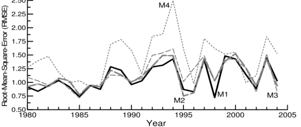
Figure 2 illustrates yearly RMSE forecasted by the 4 mod-els. The complex autoregressive model (M1) granted the smallest RMSE among the 4 models in 11 years, which is more than the other models: the M2 in 8 years, the M3 in 5 years and the M4 in 1 year, respectively. While the M1 predicted the largest RMSE among the 25-year forecasts at 1.484 in 1999, comparing to the M2 forecasted that at 1.525 in 2000, the M3 at 1.610 in 1994, and the M4 did that at 2.498 in 1994, separately. This suggests that the complex autore-gressive model (M1) gave better forecasts of the smaller and more stable RMSE than the three other models, i.e. the M1 is the best one among the 4 models. On the other hand, the persistence forecast (M4) is apparently the worst one among the 4 models in the RMSE.
As an example, Fig. 3 illustrates maps of the monthly tem-perature anomaly patterns in July 1998. The upper panel presents the forecast from the complex autoregressive model (M1), while the lower panel is the corresponding observa-tions. It shows agreements between the forecast and ob-servations: (i) positive anomalies in most areas in mainland China with errors of intensities; (ii) higher positive anoma-lies in the northern end of Northeastern China, in the area be-tween 115–120◦E and 32-37◦N, around locations at (117◦E, 26◦N), (112◦E, 27◦N) and (107◦E, 41◦N); (iii) lower pos-itive anomalies in the areas between 100–110◦E and 23-26◦N, between 86–93◦E and 28–32◦N, between 80–97◦E and 40–49◦N in China, around locations at (118◦E, 29◦N) and (107◦E, 31◦N); (iv) negative anomalies in the area of 87–88◦E and 42–45◦N, though there are wrong forecasts in smaller areas between 88–101◦E and 35–42◦N, around loca-tions at (105◦E, 38◦N), (77◦E, 39◦N), (129◦E, 42◦N) and (117◦E, 44◦N).
complex series, such as the Fourier transform and the spher-ical harmonic function.
In addition, there should be some improvements in the spa-tial pattern presentation, such as using the cluster analysis or the EOF/CEOF, instead of arranging the 160 stations in or-der of latitudes, to obtain a better result. For instance, we did forecast experiments with the M1 in a different spatial se-quence order of stations, and yielded the average ACC=0.178 in order of the original sequence number of the 160 stations, and the average ACC=0.174 in order of longitude separately. This respect is an open question to be investigated in the fu-ture.
5 Concluding remarks
In this article, the complex least-squares method was mathe-matically derived and an autoregressive model of forecasting monthly temperature anomalies was established. The appli-cation in this work shows that using a complex number to fit a meteorological element field and predicting with the com-plex autoregressive model is effective in improving the fore-cast results.
Theoretical and applied results in this study suggest that separately calculating the real and the imaginary number parts to obtain a complex least square and a complex regres-sion coefficients is a defective method.
The complex least-squares method extends the classical least-squares method from the real number domain into the complex number domain. It plays a key role and is an effec-tive method to establish complex statistic models for dealing with complex series, such as the Fourier transform and the spherical harmonic function. Other similar statistical models, such as multiple regression and nonlinear regression, may be extended from the real number domain, into complex number domain, based on the complex least-squares method. This technology perhaps may be employed to other similar ele-ment fields in the geophysical sciences.
Acknowledgements. This work is supported by the National Natural Sciences Foundation of China, #40175027, and by the Chinese Na-tional Key Program for Developing Basic Sciences, G1998040910. The authors would like to thank the referees for their ongoing support in improving this paper.
Topical Editor F. D’Andr´ea thanks two referees for their help in evaluating this paper.
References
Akaike, H.: Fitting autoregressive models for prediction, Annals Inst. Statist. Math., 27: 243–247, 1969.
Barnett, T. P.: Interaction of the monsoon and Pacific trade wind systems at interannual time scales, Part I: The equatorial Zone, Mom. Wea. Rev., 111, 756–773, 1983.
Cao, H. and Gu, X.: An integration forecast technology – Optimal harmonic method, Monthly Meteorology, 125(5), 3–6, 1999. Cao, H. and Gu, X.: An improvement upon the medium-range
Atmospheric circulation forecast with the self-memory spectral model(in Chinese), Advance in Nature Sciences, 11(3), 309–313, 2001.
Dover, T. G. J.: On the application of some stochastic models to precipitation forecasting, Quart. J. Roy.Met.Soc., 103, 177–189, 1977.
Ge, B., Shi, J., and Chou, J.: A Dynamical-statistical Long-term Weather Prediction Model Using Multi-time Historical Data, in: Preceedings of the 2nd National Conference on the Numerical Weather Prediction (in Chinese), Scieces Press, Beijing, 115– 126, 1980.
Gu, X.: A spectral model based on atmospheric self-memorization principle, Chinese Science Bulletin, 43(20), 1692–1702, 1998. Hasselmann, K. and Barnett, T. P.: Techniques of linear
predic-tion for system with periodic statistics, J. Atmos. Sci., 38, 2275– 2283, 1981.
Jiang, J.: The zonal harmonic of pentad mean 500 mb height coun-ters over the Northern Hemisphere and their prediction (in Chi-nese), Acta Meteorologica Sinica, 41(4), 433–443, 1983. Kendall, M. G. and Stuart, M.: The Advanced Theory of Statistics
I–III, Charles Griffin, London, 38–96, 1958–1976.
Kern, A. and Kern, M.: Handbook of Mathematics (in Chinese), translated by: Zhou, Q., Workers Press, Beijing, 530–534, 1987. Kleinbaum, D. G., Kupper, L. L., and Muller, K. E.: Applied Regression Analysis and Other Multivaviable Methods, PWS-KENT publishing company, Boston, 36–162, 1988.
Li, Q., Wang, N., Yi, D.: Numerical Analysis (in Chinese), Medium China Institute of Technology Press, Wuhan, 105–107, 1982. Montgomery, D. C. and Peck, E. A.: Introduction to Linear
Regres-sion Analysis, John Wiley & Sons, London, 43–85, 1982. Morrison, D. F.: Applied Linear Statistical Methods, Prentice-Hall,
Inc., Englewood Cliffs, New Jersey 07632, 228–254, 1983. Passi, R. M. and Schumann, A. P.: Autoregressive modeling of
quasi-biennial oscillation, preprints of 7th Conf. on probability and statistics in Atmos. Sci., Amer. Met. Soc., 176–181, 1984. Rasmusson, E. M., Arkin, P. A., and Chen, W. Y.: Biennial
Varia-tion in syrface temperature over the United States as revealed by singular decomposition, Mom. Wea. Rev. 109, 587–598, 1981. Sheng, J., Xie, S., and Pan, C.: Probability Theory and
Mathematic-physic Statistics (2nd version, in Chinese), Advance Education Press, Beijing, 279–290, 1995.