Prediction of dissolved reactive phosphorus losses from small agricultural catchments: calibration and validation of a parsimonious model

(1)

www.hydrol-earth-syst-sci.net/17/3679/2013/ doi:10.5194/hess-17-3679-2013

Hydrology and

Earth System

Sciences

Prediction of dissolved reactive phosphorus losses from small

agricultural catchments: calibration and validation of a

parsimonious model

C. Hahn1,2, V. Prasuhn2, C. Stamm3, P. Lazzarotto1, M. W. H. Evangelou1, and R. Schulin1

1_{ETH Zurich, Department of Environmental Systems Science, Zurich, Switzerland} 2_{Agroscope Reckenholz-Tänikon Research Station ART, Zurich, Switzerland}

3_{Eawag Swiss Federal Institute of Aquatic Science and Technology, Zurich, Switzerland}

Correspondence to:C. Hahn (claudia.hahn@env.ethz.ch)

Received: 21 December 2012 – Published in Hydrol. Earth Syst. Sci. Discuss.: 29 January 2013 Revised: 11 July 2013 – Accepted: 12 July 2013 – Published: 1 October 2013

Abstract. Eutrophication of surface waters due to diffuse phosphorus (P) losses continues to be a severe water qual-ity problem worldwide, causing the loss of ecosystem func-tions of the respective water bodies. Phosphorus in runoff often originates from a small fraction of a catchment only. Targeting mitigation measures to these critical source areas (CSAs) is expected to be most efficient and cost-effective, but requires suitable tools.

Here we investigated the capability of the parsimonious Rainfall-Runoff-Phosphorus (RRP) model to identify CSAs in grassland-dominated catchments based on readily avail-able soil and topographic data. After simultaneous calibra-tion on runoff data from four small hilly catchments on the Swiss Plateau, the model was validated on a different catch-ment in the same region without further calibration. The RRP model adequately simulated the discharge and dissolved re-active P (DRP) export from the validation catchment. Sen-sitivity analysis showed that the model predictions were ro-bust with respect to the classification of soils into “poorly drained” and “well drained”, based on the available soil map. Comparing spatial hydrological model predictions with field data from the validation catchment provided further evidence that the assumptions underlying the model are valid and that the model adequately accounts for the dominant P ex-port processes in the target region. Thus, the parsimonious RRP model is a valuable tool that can be used to deter-mine CSAs. Despite the considerable predictive uncertainty regarding the spatial extent of CSAs, the RRP can provide guidance for the implementation of mitigation measures. The

model helps to identify those parts of a catchment where high DRP losses are expected or can be excluded with high confi-dence. Legacy P was predicted to be the dominant source for DRP losses and thus, in combination with hydrologic active areas, a high risk for water quality.

1 Introduction

(2)

are (1) freshly applied fertilizers or manure (Shigaki et al., 2007; Smith et al., 2001; Vadas et al., 2011), and (2) soils that are enriched with P due to excessive fertilizer applica-tion in the past (Kleinman et al., 2011a; Vadas et al., 2005). To a much smaller extent, also plants can contribute that are freshly grazed, trampled or in decay (Kleinman et al., 2011b). Runoff from locations with freshly applied manure or high soil P concentrations bear particularly high risks for P export. Buda et al. (2009) demonstrated that even sites with relatively low soil P concentrations can deliver very high P loads when runoff is large. However, due to the complexity of the processes controlling diffuse P losses, the identifica-tion of CSAs is still difficult (Doody et al., 2012; Kleinman et al., 2011a, b).

Various tools exist to describe water and P transport from non-point sources and to identify CSAs (Radcliffe et al., 2009; Schoumans et al., 2009; Sharpley et al., 2003), rang-ing from site assessment tools such as the P index (Weld and Sharpley, 2007) to process-based dynamic models such as SWAT (Arnold et al., 1998), INCA-P (Wade et al., 2002), and ANSWERS-2000 (Beasley et al., 1980). While static models are not able to account for the temporal and spatial variability of runoff and P losses, spatially distributed dynamic models are often over-parameterized (Radcliffe et al., 2009) and re-quire many input data that are often not available. Therefore, as pointed out by Radcliffe et al. (2009), there is a need for parsimonious models that can be used to assess the spatial distribution of P export risks in a catchment. Irrespective of which type of model is used, a model requires validation for the purpose for which it is used. A major problem in validat-ing spatially localized predictions of P export from a catch-ment is that P export risks depend on processes that are sub-ject to high local spatial variability and fluctuation in time.

A parsimonious model developed to predict runoff and P losses at the outlets of small agricultural catchments is the Rainfall-Runoff-Phosphorus (RRP) model (Lazzarotto, 2005; Lazzarotto et al., 2006). The RRP model is based on the concept of spatially distributed CSAs that vary in size with hydrological conditions. It describes the export of dis-solved reactive phosphorus (DRP). This form is immediately available for algal uptake (Sharpley, 1993; Sharpley et al., 1994) and thus has a direct impact on eutrophication (Klein-man et al., 2011b). The RRP model gave a good description of discharge and DRP losses at the outlet of experimental catchments (Lazzarotto, 2005; Lazzarotto et al., 2006).

In the model it is assumed that two sites with the same topographic position belonging to the same soil type be-have the same. In order to keep the number of model pa-rameters low, the model only distinguishes between two soil types (i.e., well and poorly drained soils). This allowed for parameterizing the soil types by simultaneously calibrat-ing the model to four catchments of different soil compo-sition (Lazzarotto, 2005; Lazzarotto et al., 2006). Accord-ingly, the model should be transferable to other sites with-out calibration if the topographic and soil information is

available. Because the moisture regime is a continuum, as-signing the soils to these two classes may be somewhat arbi-trary in some cases.

In this study we investigated the validity of RRP model predictions and in particular their sensitivity on the binary classification of soils by water regime classes. First, we cali-brated the model simultaneously on runoff data of four small catchments in an agricultural area of Switzerland and then used it to predict runoff and P export from a neighboring catchment. Aside from testing the validity of these model predictions, we investigated the sensitivity of the model pre-dictions on the soil grouping and assessed the spatial per-formance of various model versions using field data on soil moisture, groundwater table, runoff volumes and P concen-trations in runoff.

2 Materials and methods

2.1 The Rainfall-Runoff-Phosphorus (RRP) model

The Rainfall-Runoff-Phosphorus (RRP) model is a parsimo-nious model for continuous simulations of DRP transport from intensively managed grassland soils into streams in small agricultural catchments. It consists of two sub-models: the semi-distributed rainfall-runoff model and the phospho-rus (P) model.

2.1.1 Rainfall-runoff sub-model

The rainfall-runoff sub-model is a soil-type-based semi-distributed model (Lazzarotto et al., 2006). It is based on the assumptions that (1) areas with the same topographic index

λand class of soil have the same hydrological behavior, and that (2) soils can be divided into two classes (i.e., well and poorly drained soils) having the same hydrologic character-istics within each class. The topographic indexλ(Beven and Kirkby, 1979; Kirkby, 1975) is defined as

λ=ln(Aupstream/tanβ), (1)

whereAupstreamis the upslope area draining through the

re-spective location (multiple flow direction algorithm of Quinn et al. (1991)) andβis the local slope at that location. It is an indicator for the wetness of the soil at a given location within the catchment. Catchments are divided into four types of hy-drological response units (HRUs) differing in runoff dynam-ics: well-drained soils (HRU1), poorly drained soils (HRU2),

urban areas (HRU3), and forests (HRU4). Soil moisture is

assumed to be uniform within each HRU. Changes in water storageSi in HRUi are calculated in hourly time steps (1t) from the mass balance equation:

(3)

runoff from HRUi during the time interval 1t. For HRU1

and HRU2the model considers two types of runoff: fast flow

qi,fast[mm] and slow flowqi,slow[mm]. The slow flow

com-ponent, which is given by

qi,slow(t )=2i(t )ci, (3)

depends (i) on the parameterci[mm] determining how much water from HRUi contributes to baseflow and (ii) on the de-gree of soil saturation2i(t )[-], which is defined as the ratio between soil water storageSi(t )[mm] and the maximum soil water storage capacitySi,max[mm]:

2i(t )= Si(t ) Si,max

. (4)

The fast flow component includes all types of quickly re-sponding flow, such as preferential flow, saturation excess and Hortonian overland flow. It is the sum of an auto-regressive part describing the recession of fast flow and of a part representing the fraction of rain directly converted into fast flow:

qi,fast(t+1t )=aiqi,fast(t )+birain(t−dti)

Ai,fast(t )

Ai

. (5)

The parameterai [–] is the fast flow decline rate,bi [–] the proportion of rain that is directly converted into fast flow, dti [h] the time delay between rainfall and runoff in HRUi, and Ai,fastA−1i the areal fraction of HRUithat contributes to fast flow. The latter depends on the soil moisture status at timet. For every time step a threshold valueλ0,i(t )[–] is determined for the topographic indexλof HRUi:

λ0,i(t )∝(1−2i(t ))ni. (6)

Locations with a topographic index higher than this thresh-old value are attributed toAi,fast [m2]. The parameterni [–] is determined by calibration. In contrast to HRU1and HRU2,

all runoff is assumed to occur as fast flow in urban areas (HRU3):

q3,fast(t+1t )=a3q3,fast(t )+b3rain(t−dt3). (7)

The total catchment response results from the sum of all flow components weighted with their respective areal frac-tionsAi/Atotal, withAtotal=PAi. Neglecting runoff from forest areas due to their limited size in the study catchments, this sum was

Q(t )=(q1,slow(t )+q1,fast(t ))

A1

Atotal

+ q2,slow(t )+q2,fast(t )

A2

Atotal

+q3,fast(t )

A3

Atotal

(8) in our case.

2.1.2 Calibration of the rainfall-runoff sub-model

Using uniform Monte Carlo simulations, the soil parameters (Table 1) were determined by simultaneous calibration of the model on four catchments (see Sect. 2.2) that differed in their soil composition and their hydrological response (Laz-zarotto et al., 2006). The calibration period extended from 7 to 17 July 2000. This short calibration period proved to be sufficient (Lazzarotto et al., 2006), as conditions varied be-tween very wet and dry. Different parameter combinations were generated using random sampling within the domain of each parameter. The following Nash–Sutcliffe criterion (NSC) (Nash and Sutcliffe, 1970), calculated for the four catchments together, was used to assess model performance of each parameter combination:

NSC=1−

P4

k=1

Pte t=t0(Q

k

obs(t )−Qksim(t ))2

P4

k=1

Pte t=t0(Q

k

obs(t )− ¯Q

k

obs)2

, (9)

whereQobs(t )[mm] is the observed runoff at timet,Qsim(t )

[mm] the simulated runoff at timet, andQ¯obs[mm] the mean

observed runoff for the whole time period in catchmentk. The evaluated parameter sets were classified as either “be-havioral” (or “accepted”) for NSC>NSCthreshold or

“non-behavioral” for NSC<NSCthreshold (Hornberger and Spear,

1981). Behavioral parameter sets were used for model ap-plication. Thus, the number of accepted parameter sets (mc) defines the number of simulation results. The 10 % quantiles and 90 % quantiles of these simulations were used to charac-terize the uncertainty of the model predictions.

For more information on the hydrological model, the reader is referred to Lazzarotto et al. (2006). Here, we con-verted the model from FORTRAN77 to FORTRAN95 in or-der to make a few modifications (such as corrections of some coding errors and removal of parameter constraints). We will refer to this version of this model in which all soil param-eters were calibrated simultaneously as Version 1. In a sec-ond model version (Version 2) the urban parametersa3and

b3 were separately calibrated using discharge data from six

small runoff events in July 2010 recorded in the Stägbach catchment, which is located in the vicinity of the calibration catchments (see Sect. 2.2). As soil moisture was low prior to these six events, runoff from agricultural land could be neglected. The resulting parameter values werea3=0.0968

andb3=0.0894. The third model version (Version 3) was

identical to Version 2, but used a different soil classification (see Sect. 2.3.1).

(4)

Table 1.Parameters of the hydrological response units (HRUi= 1, 2, 3) that need to be determined during calibration (adopted from Table 2 in Lazzarotto et al., 2006). HRU1= well drained, HRU2= poorly drained, HRU3= urban.

Global Minimum Maximum

parameter value value Property Used HRU

S_i,max[mm] 0 800 Maximum soil water storage capacity i=1, 2

ai [–] 0 1 Fast flow decline rate i=1, 2, 3

bi [–] 0 1 Proportion of rainfall converted into fast i=1, 2, 3

flow on the contributing areas

ci[mm] 0 1 Flow rate between the scaled soil water i=1, 2

storage and the slow flow components

ni[–] 1 10 Expansion control of areas contributing to fast flow i=1, 2

2.1.3 The phosphorus model

The Phosphorus (P) sub-model was developed to predict DRP losses at catchment outlets and CSAs within catch-ments in combination with the rainfall-runoff sub-model (Lazzarotto, 2005). The model was developed for the Lip-penrütibach catchment, a catchment on the Swiss Plateau, which was also used for calibration of the hydrological sub-model. Previous studies in the study region had shown that DRP concentrations in runoff were strongly correlated with runoff volume (Lazzarotto et al., 2005; Pacini and Gächter, 1999; Stamm et al., 1998), indicating that high rates of P losses were associated with fast runoff. To account for the elevated P concentrations of fast runoff as compared to slow runoff, fast flow is assumed to be composed of “old” and “new” water, while slow flow is assumed to consist of “old” water only. While qi,slow(t ) and qi,fast(t ) are average

val-ues that apply to all cells within an HRUi, the P sub-model distinguishes between grid cells within the respective HRUi that actually contribute to fast flow in a given event and cells that do not, assuming that total fast flow is equally dis-tributed among the cells that contribute. Thus, for cells that contribute fast flow qi,fast(t, x, y) is calculated by dividing

qi,fast(t )by the areal fraction (Ai,fast(t )/Ai) of HRUi that contributes to fast flow, while fast flowqi,fast(t, x, y) from

cells that are not contributing is zero. The new water compo-nent,qi,new(t, x, y)[mm], is assumed to be a constant

frac-tionη [–] of the total fast flow from the contributing area:

qi,new(t, x, y)=η qi,fast(t )

Ai Ai,fast(t )

F (t, x, y), (10)

whereF (t, x, y)is 0 for cells not contributing to fast flow, and 1 for cells contributing to fast flow at timet, andxandy

are the central coordinates of the respective cell. The fraction

ηwas estimated from nitrate dilution data collected during runoff events and baseflow conditions as 0.25±0.05 (Laz-zarotto, 2005). The flow of old water [mm] is the sum of the remaining fast flow and the slow flow of the respective cell:

qi,old(t, x, y)=(1−η) qi,fast(t )

Ai

Ai,fast(t )

F (t, x, y)+qi,slow(t ). (11)

The DRP loss with old water flow is calculated for every grid cell as

Li,old(t, x, y)=DRPbaseflowqi,old(t, x, y)gridsize, (12)

assuming that the concentration of DRP in old water is the same as the DRP concentration of the baseflow, DRPbaseflow

(0.05 mg L−1). DRP losses associated with new water flow include incidental P losses from freshly applied manure (DRPIPL [mg L−1]) and P losses from soil (DRPsoil [mg

L−1]) enriched in P due to excessive manure applications in the past. DRPsoilconcentrations were calculated for every

pixel from water-soluble soil P (WSP) concentrations. The WSP–DRP relationship was taken from artificial rainfall ex-periments carried out in the catchment area of Lake Baldegg (Hahn et al., 2012).

DRP[mgL−1] =0.0852WSP[mgkg−1] −0.3039, (13) with the condition that no negative DRP values can occur. The WSP concentrations (and thus also the DRPsoil

concen-trations) were assumed to remain constant over the simula-tion period in the present study.

In contrast, DRPIPL(t, x, y)concentrations in runoff were

considered to vary in time. Based on the studies of Braun et al. (1993) and Von Albertini et al. (1993), DRPIPL(t, x, y)

is assumed to decrease exponentially with increasing time lag1tm=tr−tabetween manure applicationtaand onset of

runofftr:

DRPIPL(t, x, y)=DRP0IPL(t, x, y)exp(−1tmh) (14)

The timetof runoff onset is the time when the respective soil pixel starts to contribute to fast flow (Lazzarotto, 2005). The parameterhwas assumed to be the same for well and poorly drained soils: 0.007±0.004. The value range of parameter

h was determined preliminary, by fitting the DRPIPL

func-tion to observed data (Lazzarotto, 2005). With each applica-tion of manure 1tm is set to zero, and the DRPIPL(t, x, y)

(5)

The total DRP load [mg] associated with new water is the sum of DRPsoiland DRPIPLloss at each pixel:

Li,new(t, x, y)=(DRPsoil(x, y)

+DRPIPL(t, x, y)) qi,new(t, x, y)gridsize (15)

while the total DRP loss from a pixel at timetis the sum of

Li,old(t, x, y)+Li,new(t, x, y), and the total loss of DRP from

the catchment is the sum of DRP loss from all soil pixels. We used Gaussian error propagation to account for uncer-tainty in the model parametersηandhand in the WSP–DRP relationship. Thus, for each mc model run and time step we obtained an error estimate. These were combined with the 10 % and 90 % quantiles of the hydrological predictions to give the uncertainty of the DRP export predictions.

2.2 Study area

The study area was situated on the Swiss Plateau in the vicin-ity of Lucerne. It is characterized by undulating terrain, rang-ing between 500 and 800 m altitude above sea level and cov-ered by glacial tills (Lazzarotto et al., 2006). The soils are generally loamy and of low permeability (Peyer et al., 1983). Average amounts of annual precipitation in the region range between 1000 and 1200 mm, depending primarily on alti-tude.

The four catchments used for model calibration (Lippen-rütibach (LIP), Greuelbach (GRB), Rotbach (RTB), Meien-bach (MEI)) drain into Lake Sempach (Lazzarotto, 2005), whereas the catchment (Stägbach catchment (Stäg)) used for model validation drains into Lake Baldegg (Fig. 1). Both lakes have serious eutrophication problems and are artifi-cially aerated. The region is characterized by intensive ani-mal husbandry (dairy and pig farms, 2.4 livestock units per ha (Herzog, 2005)), which in the past has resulted in highly increased soil P stocks (Stamm et al., 1998).

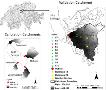
In addition to the Stägbach catchment as a whole, we also used a sub-catchment of the Stägbach catchment, denoted as Stäg2, for validation (Fig. 1). Table 2 shows that the percent-ages of urban area, forest, and agricultural area in the vali-dation catchments were in the range of the calibration ments. Agriculture is the dominating land use in all catch-ments, whereas the area classified as urban covered less than 10 %. The latter consisted of a few villages and some iso-lated farms. While the Stäg2 sub-catchment was compara-ble in size to the calibration catchments, the Stägbach catch-ment as a whole (8.24 km2) was larger than all four calibra-tion catchments. More informacalibra-tion on the calibracalibra-tion catch-ments is given by Lazzarotto et al. (2006). Small differences between the HRU percentiles given here and those by Laz-zarotto et al. (2006) are due to the fact that the data had to be processed anew.

Fig. 1.Locations of calibration and validation catchments and the installed measurement devices.

2.3 Model validation

2.3.1 Model input data

Precipitation and evapotranspiration

From April till October 2010 a weather station was installed in the center of the Stägbach catchment to obtain representa-tive precipitation data for the Stägbach catchment. The sta-tion was equipped with a R102/R102H tipping bucket rain gauge. Data were recorded every 15 min. For two short time periods (28 May–8 June 2010 and 21 July–1 August 2010), no data were recorded at this weather station, due to tech-nical problems. For these periods we used precipitation data from the nearest weather station (Hochdorf, data from uwe in the canton of Lucerne), which is located less than 2 km away from the Stägbach catchment. All other data gaps were filled with mean precipitation data from the three closest weather stations (Buchs, Lucerne, Cham, provided by the Swiss Fed-eral Office of meteorology and Climatology) surrounding the catchment. Two Hellmann rain gauges were installed in the catchment to check for spatial variability in rainfall. For the global radiation data, we used evapotranspiration data from the three weather stations Buchs, Lucerne and Cham (pro-vided by the Swiss Federal Office of meteorology and Clima-tology). These data are based on the Primault formula. They were available at daily resolution, but using mean global ra-diation data from the same three MeteoSwiss stations, we derived estimates of hourly evapotranspiration.

Topographic index and HRU determination

(6)

Table 2.Areal fraction of each hydrological response unit (HRU) on the total catchment area in [%] – roman font = model Version 2, bold font = model Version 3.

Calibration catchments Validation catchments

LIP LIP RTB RTB MEI MEI GRB GRB Stäg Stäg Stäg2 Stäg2

Urban [%] 8.1 8.1 9 8.7 2.5 2.5 8 7.6 9 9 6 6

Forest 16.7 16.7 16 16.4 7.7 7.7 16 16.3 8 8 9.5 9.5

Well 38.6 13.1 56 31.5 74 40.6 61 34.6 66 42 67.2 41.2

Poor 36.6 62.1 19 43.4 15.8 49.2 15 41.5 17 41 17.3 43.3

Area [km2] 3.3 6.0 1.2 2.6 8.24 2.27

which is available for the whole of Switzerland (provided by the Swiss Federal Office of Topography), using the open source GIS software Saga 2.0. The convergence coefficient was set to 1. Urban areas and forests were identified us-ing aerial photographs (provided by the Swiss Federal Of-fice of Topography). The data were processed and prepared for model input using ArcGIS (ArcGIS Desktop 10 Service Pack 2, ESRI) and the software package R (RDevelopment-CoreTeam, 2007).

Soil classification into drainage classes

The assignment of soils to the two classes of well and poorly drained soils was based on the local soil map (Peyer et al., 1983). In model Version 1 and 2 we followed Lazzarotto et al. (2006), who classified Eutric and Dystric Cambisols and Eutric Regosols as well-drained soils and Gleyic Cam-bisols and Eutric Gleysols as poorly drained soils. To inves-tigate the sensitivity of the model to this classification, we compared Version 2 with Version 3. In the latter we also assigned soils considered well drained by Lazzarotto et al. (2006), although showing signs of temporary water stagna-tion or water-logging according to the soil map, to the poorly drained soils. Accordingly the areal fraction occupied by the poorly drained HRU was larger in Version 3 than in Version 1 and 2 (Table 2).

Soil P status and manure application

A map of the spatial distribution of soil P concentrations (see Fig. S1) was constructed from data of soil P analyses farmers have to provide to local authorities every 5 yr. With the help of the farmers, the available data on soil P status were as-signed to individual fields. Some farmers did not cooperate. In these cases we used P data obtained from the environmen-tal protection agency of the canton of Lucerne and attributed area-weighted mean P values to the respective management units.

Some farmers also provided detailed data on the amounts, locations and times of manure application on their farms. For the other farms, which covered more than 80 % of the

area, the manure P pool was neglected. In contrast, manure application data were complete for the Lippenrütibach catch-ment, one of the calibration catchments, in the year 1999. 2.3.2 Model validation

Discharge measurements

At the outlet of the Stägbach catchment, a 6712 Full-size Portable Sampler (ISCO, USA) was used to determine dis-charge and collect water samples. In addition, the water level was recorded every minute by means of a Bubbler Flow Module. Further flow and water level measurements (dilu-tion method) were taken by a consulting company (Büro für Wasser und Umwelt, BWU) working for the cantonal en-vironmental protection agency. They provided us also with the level–discharge data necessary to calculate the discharge from the level data.

(7)

Water samples

Using the aforementioned 6712 Full-size Portable Sampler, flow-proportional water samples were collected automati-cally at the outlet of the Stägbach catchment and the Stäg2 sub-catchment. A pre-defined water level (Stäg) or flow ve-locity (Stäg2 sub-catchment) threshold was set, and when it was reached, samples were taken automatically every 15 min. Four subsequent samples were collected in the same bottle, resulting in one composite sample every hour, as long as the water level (or the velocity, respectively) was above the threshold. After a runoff event, samples were collected and stored at 4◦C till analysis. In addition, we took grab samples each time we went into the field, at least once a week. Dis-solved reactive phosphorus (DRP) was analyzed by means of the molybdate colorimetry method (Vogler, 1965) after fil-tration (<450 nm) of sample solution. In order to determine total phosphorus (TP), unfiltered samples were digested in potassium persulfate before they were analyzed for P using the molybdate colorimetry method. Electrical conductivity (EC) was measured using a Metrohm Conductometer 712. Soil moisture measurements

On four grassland sites (Table 3) soil water content was mon-itored at 10 and 30 cm depth using six horizontally inserted 2-rod TDR probes at each depth. The signal was recorded by means of a TDR100 and stored by a data logger (CR10X, Campbell Scientific, Inc.). The volumetric soil water content (m3_m−3_{) was calculated using the equation given by Topp}

et al. (1980). Volumetric soil samples were taken at each of the four soil water monitoring locations using steel cylinders to determine soil bulk density and porosity.

Piezometer and overland flow detectors

Furthermore, we installed a piezometer equipped with a light plummet and an overland flow detector (OFD; see Doppler et al., 2012) at each soil water monitoring station and 6 other locations. Readings of these instruments were taken approx-imately once a week normally and more often after rainfall events.

3 Results

3.1 Model performance at the catchment outlet

3.1.1 The rainfall-runoff model

Model calibration with data from the year 2000

Without separate calibration of the urban parameters (Ver-sion 1), the model performed poorly. Out of 7 million Monte Carlo (MC) simulations, no parameter set achieved a NSC value>0.5; 661 parameter sets yielded a NSC>0.4. Sepa-rate calibration of the urban parameters (Version 2) improved

the model results substantially and resulted in 724 accepted parameter sets from 5 million MC runs when the threshold value was set to 0.6, with 25 %, 50 %, and 75 % quantiles of 0.61, 0.61 and 0.63, respectively. Changing the classification of the soils (Version 3) decreased the performance for the cal-ibration period, so that the NSC threshold had to be reduced to 0.5 to obtain 606 accepted parameter sets, with 25 %, 50 % and 75 % NSC quantiles of 0.51, 0.52 and 0.53 respectively. Comparison of predictions for the Lippenrütibach catchment

Before we applied the calibrated model to the Stägbach catchment, we compared hydrological predictions for the Lippenrütibach catchment (LIP), one of the calibration catch-ments, for the year 1999. The same data had been used for validation by Lazzarotto et al. (2006). Figure 2a shows a fair agreement between simulations (Version 2) and measure-ments. Predictions were again better for the model version with separate calibration of the urban HRU parametersa3

andb3(Version 2) than for the corrected original version of

the model (Version 1) (Table 4). This improvement was in particular due to better prediction of small peaks, which were overestimated by the original model (Lazzarotto et al., 2006). However, two other problems, which had already been identi-fied by Lazzarotto et al. (2006), remained unsolved: (1) some high runoff peaks were still underestimated, and (2) baseflow declined too fast after long periods with no rainfall (Fig. 2b). Model validation – Stägbach 2010

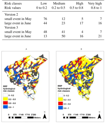
To test how well the model performs when applied outside the watersheds used for calibration, we applied the calibrated Version 2 model to the Stägbach catchment for a forward prediction of discharge during the year 2010 and compared predictions with measurements. Figures 3 and 4 show that the model performed well for the entire catchment as well as for the Stäg2 sub-catchment. The median NSC values were 0.62 and 0.72, respectively (Table 4). With the global pa-rameter cwell ranging mainly between 0.7 and 0.92 (25 %

and 75 % quantiles), and cpoor ranging between 0.33 and

(8)

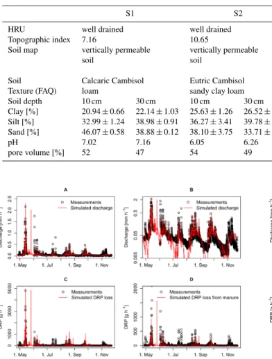
Table 3.Site characteristics of the four permanent measurement stations in the Stägbach catchment.

S1 S2 S3 S4

HRU well drained well drained poorly drained well drained

Topographic index 7.16 10.65 11.13 7.27

Soil map vertically permeable vertically permeable ground-/slope vertically permeable

soil soil water-dominated soil soil, partly ground- or

slope water-influenced Soil Calcaric Cambisol Eutric Cambisol Eutric Cambisol Eutric Cambisol

Texture (FAQ) loam sandy clay loam loam loam

Soil depth 10 cm 30 cm 10 cm 30 cm 10 cm 30 cm 10 cm 30 cm

Clay [%] 20.94±0.66 22.14±1.03 25.63±1.26 26.52±2.11 25.25±0.13 19.62±0.35 17.80±1.39 18.99±2.27 Silt [%] 32.99±1.24 38.98±0.91 36.27±3.41 39.78±0.09 46.39±0.82 44.03±0.56 32.40±0.47 35.03±0.2 Sand [%] 46.07±0.58 38.88±0.12 38.10±3.75 33.71±2.02 28.36±0.95 36.34±0.21 49.80±0.92 45.97±2.07

pH 7.02 7.16 6.05 6.26 5.32 5.45 5.89 6.59

pore volume [%] 52 47 54 49 41 41 53 44

Fig. 2.Simulations (lines, 10 % and 90 % quantiles) using RRP Ver-sion 2 versus measured (points) discharge and DRP loss from the Lippenrütibach catchment in 1999. Theyaxes in figures on the right are in logarithmic scale (B) or focus on a certain part of the value range (D).(C)shows the total range of the DRP loads measured and simulated on a non-log scale.

126 mm rain while the other one only collected 88 mm within the same time frame.

Influence of soil classification – model Version 3

As in the calibration, Version 3 did not perform as well as Version 2 also in the validation for the Lippenrütibach catch-ment (Table 4), as runoff peaks were slightly lower in simu-lations with Version 3 than with Version 2. The higher value ofcpoorand the higher areal percentage of HRUpoor(62.1 %)

resulted in higher slow flow from poorly drained soils, which led to lower soil moisture and thus to lower peak flows. In contrast, the change in soil classification from Version 2 to Version 3 improved model predictions for the entire Stäg-bach catchment and the Stäg2 sub-catchment (Table 4). The improvement was due to better simulations of baseflow and of the large runoff event in June. This can be attributed to

0.0

1.0

2.0

3.0

Discharge [mm h

− 1] ● ●●●●●●●●●●●●●●●●●●●●●●●●●●●●●●●●●●●●●●●●●●●●●●●●●●●●●●●●●●●●●●●●●●●●●●●●●●●●●●●●●●●●●●●●●●●●●●●●●●●●●●●●●●●●●●●●●●●●●●●●●●●●●●●●●●●●●●●●●●●●●●●●●●●●●●●●●●●●●●●●●●●●●●●●●●●●●●●●●●●●●●●●●●●●●●●●●●●●●●●●●●●●●●●●●●●●●●●●●●●●●●●●●●●●●●●●●●●●●●●●●●●●●●●●●●●●●●●●●●●●●●●●●●●●●●●●●●●●●●●●●●●●●●●●●●●●●●●●●●●●●●●●●●●●●●●●●●●●●● ● ● ● ● ● ●●●●●●●●●●●●●●●●●●●●●●●●●●●●●●●●●●●●●●●●●●●●●●●●●●●●●●●●●●●●●●●●●●●●●●●●●●●●●●●●●●●●●●●●●●●●●●●●●●●●●●●●●●●●●●●●●●●●●●●●●●●●●●●●●●●●●●●●●●●●●●●●●●●●●●●●●●●●●●●●●●●●●●●●●●●●●●●●●●●●●●●●●●●●●●●●●●●●●●●●●●●●●●●●●●●●●●●●●●●●●●●●●●●●●●●●●●●●●●●●●●●●●●●●●●●●●●●●●●●●●●●●●●●●●●●●●●●●●●●●●●●●●●●●●●●●●●●●●●●●●●●●●●●●●●●●●●●●●●●●●●●●●●●●●●●●●●●●●●●●●●●●●●●●●●●●●●●●●●●●●●●●●●●●●●●●●●●●●●●●●●●●●●●●●●●●●●●●●●●●●●●●●●●●●●●●●●●●●●●●●●●●●●●●●●●●●●●●●●●●●●●●●●●●●● ● ● ● ● ● ● ● ●●●●●●●●●●●●●●●●●●●●●●●●●●●●●●●●●●●●●●●●●●●●●●●●●●●●●●●●●●●●●●●●●●●●●●●●●●●●●●●●●●●●●●●●●●●●●●●●●●●●●●●●●●●●●●●●●●●●●●●●●●●●●●●●●●●●●●●●●●●●●●●●●●●●●●●●●●●●●●●●●●●●●●●●●●●●●●●●●●●●●●●●●●●●●●●●●●●●●●●●●●●●●●●●●●●●●●●●●●●●●●●●●●●●●●●●●●●●●●●●●●●●●●●●●●●●●●●●●●●●●●●●●●●●●●●●●●●●●●●●●●●●●●●●●●●●●●●●●●●●●●●●●●●●●●●●●●●●●●●●●●●●●●●●●●●●●●●●●●●●●●●●●●●●●●●●●●●●●●●●●●●●●●●●●●●●●●●●●●●●●●●●●●●●●●●●●●●●●●●●●●●●●●●●●●●●●●●●●●●●●●●●●●● ● ● ● ● ● ● ● ● ● ● ● ● ● ● ● ● ● ● ● ● ● ●●●●●●●●●●●●●●●●● ● ● ● ● ● ● ● ● ● ● ● ● ● ● ● ● ● ● ● ● ●●●●●●●●●●●●●●●●●●●●●●●●●●●●●●●●●●●●●●●●●●●●●●●●●●●●●●●●●●●●●●●●●●●●●●●●●●●●●●●●●●●●●●●●●●●●●●●●●●●●●●●●●●●●●●●●●●●●●●●●●●●●●●●●●●●●●●●●●●●●●●●●●●●●●●●●●●●●●●●●●●●●●●●●●●●●●●●●●●●●●●●●●●●●●●●●●●●●●●●●●●●●●●●●●●●●●●●●●●●●●●●●●●●●●●●●●●●●●●●●●●●●●●●●●●●●●●●●●●●●●●●●●●●●●●●●●●●●●●●●●●●●●●●●●●●●●●●●●●●●●●●●●●●●●●●●●●●●●●●●●●●●●●●●●●●●●●●●●●●●●●●●●●●●●●●●●●●●●●●●●●●●●●●●●●●●●●●●●●●●●●●●●●●●●●●●●●●●●●●●●●●●●●●●●●●●●●●●●●●●●●●●●●●●●●●●●●●●●●●●●●●●●●●●●●●●●●●●●●●●●●●●●●●●●●●●●●●●●●●●●●●●●●●●●●●●●●●●●●●●●●●●●●●●●●●●●●●●●●●●●●●●●●●●●●●●●●●●●●●●●●●●●●●●●●●●●●●●●●●●●●●●●●●●●●●●●●●●●●●●●●●●●●●●●●●●●●●●●●●●●●●●●●●●●●●●●●●●●●●●●●●●●●●●●●●●●●●●●●●●●●●●●●●●●●●●●●●●●●●●●●●●●●●●●●●●●●●●●●●●●●●●●●●●●●●●●●●●●●●●●●●●●●●●●●●●●●●●●●●●●●●●●●●●●●●●●●●●●●●●●●●●●●●●●●●●●●●●●●●●●●●●●●●●●●●●●●●●●●●●●●●●●●●●●●●●●●●●●●●●●●●●●●●●●●●●●●●●●●●●●●●●●●●●●●●●●●●●●●●●●●●●●●●●●●●●●●●●●●●●●●●●●●●●●●●●●●●●●●●●●●●●●●●●●●●●●●●●●●●●●●●●●●●●●●●●●●●●●●●●●●●●●●●●●●●●●●●●●●●●● ● ● ● ● ● ● ● ● ● ● ● ● ● ● ● ● ● ● ●●●●●●●●●●●●●●●●●●●●●●●●●●●●●●●●●●●●●●●●●●●●●●●●●●●●●●●●●●●●●●●●●●●●●●●●●●●●●●●●●●●●●●●●●●●●●●●●●●●●●●●●●●●●●●●●●●●●●●●●●●●●●●●●●●●●●●●●●●●●●●●●●●●●●●●●●●●●●●●●●●●●●●●●●●●●●●●●●●●●●●●●●●●●●●●●●●●●●●●●●●●●●●●●●●●●●●●●●●●●●●●●●●●●●●●●●●●●●●●●●●●●●●●●●●●●●●●●●●●●●●●●●●●●●●●●●●●●●●●●●●●●●●●●●●●●●●●●●●●●●●●●●●●●●●●●●●●●●●●●●●●●●●●●●●●●●●●●●●●●●●●●●●●●●●●●●●●●●●●●●●●●●●●●●●●●●●●●●●●●●●●●●●●●●●●●●●●●●●●●●●●●●●●●●●●●●●●●●●●●●●●●●●●●●●●●●●●●●●●●●●●●●●●●●●●●●●●●●●●●●●●●●●●●●●●●●●●●●●●●●●●●●●●●●●●●●●●●●●●●●●●●●●●●●●●

1. May 1. Jun 1. Jul 1. Aug

● Simulation Measurements ●● ●●●● ● ●●●●●●●●●●●●●●●●●●●●●●●●● ● ● ● ● ●●●●●●●●●●● ●●●●●●●●● ● ●●● ●●●●●●●●●●●●●●●●●●●●●●●●● ● ● ● ● ● ● ● ● ● ● ● ● ● ●● ●● ●● ● ●●●● ●●● ● ● ● ● ● ● ● ●●●●●●●●●●●●●● ●●●●●●● 0 2000 6000 10000

DRP [g h

−

1]

● Simulation Measurements

Fig. 3.Simulations (lines, 10 % and 90 % quantiles) using RRP Ver-sion 2 versus measured (points) discharge and DRP loss from the Stägbach catchment in 2010.

the lower value ofcwell(25 % and 75 % quantiles: 0.31, 0.75)

and the lower areal fraction of well-drained soils in Version 3 (Table 2), resulting in higher soil moisture and consequently also in higher peak flows. The larger area of poorly drained soils also led to steeper decline of the hydrographs (Fig. 5), due to a larger contribution of the poorly drained HRU to fast flow. Apart from these rather small differences, both versions of the model simulated the discharge dynamics of the study catchments quite well.

3.1.2 The phosphorus model

(9)

Table 4.Performance of different model versions in three catchments (Lippenrütibach catchment (LIP), Stägbach catchment (Stäg), Stägbach sub-catchment (Stäg2)), measured with the Nash–Sutcliffe criterion (NSC) (Nash and Sutcliffe, 1970). Version 1 – corrected original model, Version 2 – separate urban parameter calibration, Version 3 – separate urban parameter calibration + different soil classification.

Lip Stäg Stäg2

Model version NSC quantiles Calibration

25 % 50 % 75 % 25 % 50 % 75 % 25 % 50 % 75 % NSC_threshold

Version 1 0.42 0.44 0.46 0.50 0.61 0.70 0.65 0.71 0.78 0.4

Version 2 0.48 0.50 0.52 0.53 0.62 0.71 0.66 0.72 0.80 0.6

Version 3 0.44 0.46 0.48 0.62 0.68 0.75 0.68 0.74 0.80 0.5

0.0

1.0

2.0

Discharge [mm h

− 1] ● ●●●●●●●●●●●●●●●●●●●●●●●●●●●●●●●●●●●●●●●●●●●●●●●●●●●●●●●●●●●●●●●●●●●●●●●●●●●●●●●●●●●●●●●●●●●●●●●●●●●●●●●●●●●●●●●●●●●●●●●●●●●●●●●●●●●●●●●●●●●●●●●●●●●●●●●●●●●●●●●●●●●●●●●●●●●●●●●●●●●●●●●●●●●●●●●●●●●●●●●●●●●●●●●●●●●●●●●●●●●●●●●●●●●●●●●●●●●●●●●●●●●●●●●●●●●●●●●●●●●●●●●●●●●●●●●●●●●●●●●●●●●●●●●●●●●●●●●●●●●●●●●●●●●●●●●●●●●●●● ● ● ● ●●●●●●●●●●●●●●●●●●●●●●●●●●●●●●●●●●●●●●●●●●●●●●●●●●●●●●●●●●●●●●●●●●●●●●●●●●●●●●●●●●●●●●●●●●●●●●●●●●●●●●●●●●●●●●●●●●●●●●●●●●●●●●●●●●●●●●●●●●●●●●●●●●●●●●●●●●●●●●●●●●●●●●●●●●●●●●●●●●●●●●●●●●●●●●●●●●●●●●●●●●●●●●●●●●●●●●●●●●●●●●●●●●●●●●●●●●●●●●●●●●●●●●●●●●●●●●●●●●●●●●●●●●●●●●●●●●●●●●●●●●●●●●●●●●●●●●●●●●●●●●●●●●●●●●●●●●●●●●●●●●●●●●●●●●●●●●●●●●●●●●●●●●●●●●●●●●●●●●●●●●●●●●●●●●●●●●●●●●●●●●●●●●●●●●●●●●●●●●●●●●●●●●●●●●●●●●●●●●●●●●●●●●●●●●●●●●●●●●●●●●●●●●●●●●●●●●●●●●●●●●●●●●●●●●●●●●●●●●●●●●●●●●●●●●●●●●●●●●●●●●●●●●●●●●●●●●●●●●●●●●●●●●●●●●●●●●●●●●●●●●●●●●●●●●●●●●●●●●●●●●●●●●●●●●●●●●●●●●●●●●●●●●●●●●●●●●●●●●●●●●●●●●●●●●●●●●●●●●●●●●●●●●●●●●●●●●●●●●●●●●●●●●●●●●●●●●●●●●●●●●●●●●●●●●●●●●●●●●●●●●●●●●●●●●●●●●●●●●●●●●●●●●●●●●●●●●●●●●●●●●●●●●●●●●●●●●●●●●●●●●●●●●●●●●●●●●●●●●●●●●●●●●●●●●●●●●●●●●●●●●●●●●●●●●●●●●●●●●●●●●●●●●●●●●●●●●●●●●●●●●●●●●●●●●●●●●●●●●●●●●●●●●●●●●●●●●●●●●●●●●●●●●●●●●●●●●●●●●●●●●●●●● ● ● ● ● ● ● ● ● ● ● ● ● ● ● ● ● ● ● ● ● ● ● ● ● ● ● ●●●●●●●●●●●● ● ● ● ● ● ● ●●●● ● ● ● ● ● ● ●●●●●●●●●●●●●●●●●●●●●●●●●●●●●●●●●●●●●●●●●●●●●●●●●●●●●●●●●●●●●●●●●●●●●●●●●●●●●●●●●●●●●●●●●●●●●●●●●●●●●●●●●●●●●●●●●●●●●●●●●●●●●●●●●●●●●●●●●●●●●●●●●●●●●●●●●●●●●●●●●●●●●●●●●●●●●●●●●●●●●●●●●●●●●●●●●●●●●●●●●●●●●●●●●●●●●●●●●●●●●●●●●●●●●●●●●●●●●●●●●●●●●●●●●●●●●●●●●●●●●●●●●●●●●●●●●●●●●●●●●●●●●●●●●●●●●●●●●●●●●●●●●●●●●●●●●●●●●●●●●●●●●●●●●●●●●●●●●●●●●●●●●●●●●●●●●●●●●●●●●●●●●●●●●●●●●●●●●●●●●●●●●●●●●●●●●●●●●●●●●●●●●●●●●●●●●●●●●●●●●●●●●●●●●●●●●●●●●●●●●●●●●●●●●●●●●●●●●●●●●●●●●●●●●●●●●●●●●●●●●●●●●●●●●●●●●●●●●●●●●●●●●●●●●●●●●●●●●●●●●●●●●●●●●●●●●●●●●●●●●●●●●●●●●●●●●●●●●●●●●●●●●●●●●●●●●●●●●●●●●●●●●●●●●●●●●●●●●●●●●●●●●●●●●●●●●●●●●●●●●●●●●●●●●●●●●●●●●●●●●●●●●●●●●●●●●●●●●●●●●●●●●●●●●●●●●●●●●●●●●●●●●●●●●●●●●●●●●●●●●●●●●●●●●●●●●●●●●●●●●●●●●●●●●●●●●●●●●●●●●●●●●●●●●●●●●●●●●●●●●●●●●●●●●●●●●●●●●●●●●●●●●●●●●●●●●●●●●●●●●●●●●●●●●●●●●●●●●●●●●●●●●●●●●●●●●●●●●●●●●●●●●●●●●●●●●●●●●●●●●●●●●●●●●●●●●●●●●●●●●●●●●●●●●●●●●●●●●●●●●●●●●●●●●●●●●●●●●●●●●●●●●●●●●●●●●●●●●●●●●● ● ● ● ● ● ● ● ● ● ● ● ● ● ● ●●●●●●●●●●●●●●●●●●●●●●●●●●●●●●●●●●●●●●●●●●●●●●●●●●●●●●●●●●●●●●●●●●●●●●●●●●●●●●●●●●●●●●●●●●●●●●●●●●●●●●●●●●●●●●●●●●●●●●●●●●●●●●●●●●●●●●●●●●●●●●●●●●●●●●●●●●●●●●●●●●●●●●●●●●●●●●●●●●●●●●●●●●●●●●●●●●●●●●●●●●●●●●●●●●●●●●●●●●●●●●●●●●●●●●●●●●●●●●●●●●●●●●●●●●●●●●●●●●●●●●●●●●●●●●●●●●●●●●●●●●●●●●●●●●●●●●●●●●●●●●●●●●●●●●●●●●●●●●●●●●●●●●●●●●●●●●●●●●●●●●●●●●●●●●●●●●●●●●●●●●●●●●●●●●●●●●●●●●●●●●●●●●●●●●●●●●●●●●●●●●●●●●●●●●●●●●●●●●●●●●●●●●●●●●●●●●●●●●●●●●●●●●●●●●●●●●●●●●●●●●●●●●●●●●●●●●●●●●●●●●●●●●●●●●●●●●●●●●●●●●●●●●●●●●●●●●●●●●

● Simulation Measurements ● ●● ●● ●● ●● ● ● ● ● ● ● ● ● ● ● ● ● ● ● ● ● ● ● ● ● ● ● ● ●●●●●●●●●●●● ●●●●●●● ●●●●●●●●●●●●●●●●●●●●●●●● ●● ● ●● ● ●● ● 0 1000 3000

DRP [g h

−

1]

Fig. 4.Simulations (lines, 10 % and 90 % quantiles) using RRP Ver-sion 2 versus measured (points) discharge and DRP loss from the Stägbach sub-catchment (Stäg2) in 2010.

for which runoff was underestimated as well. On the other hand discharge and DRP load were well predicted for the large events in May 1999 (Lippenrütibach) and in June 2010 (Stägbach). As the simulated water fluxes match the observed water fluxes most of the time quite well, a good match of the observed DRP losses implies that also the DRP concentra-tions are matched well. Unfortunately, in the Stägbach catch-ments no samples were collected during the second peak of the extreme event because the sampling device was either clogged (Stäg) or dislocated (Stäg2).

The simulated loss of DRP from the Lippenrütibach catchment that was attributable to recently applied manure (Fig. 2d) was about 1/5 of the total DRP loss (Fig. 2c) dur-ing the large event in May, and less than half of the total simulated DRP load in most of the other events. Thus, most DRP lost with runoff came from the soils according to the model. In the Stägbach catchments, a good fit between sim-ulations and measurements was obtained despite the limited availability of manure application data, suggesting again that soil P was the main source for the DRP losses with runoff.

0.0

1.0

2.0

3.0

Discharge [mm h

− 1] ● ●●●●●●●●●●●●●●●●●●●●●●●●●●●●●●●●●●●●●●●●●●●●●●●●●●●●●●●●●●●●●●●●●●●●●●●●●●●●●●●●●●●●●●●●●●●●●●●●●●●●●●●●●●●●●●●●●●●●●●●●●●●●●●●●●●●●●●●●●●●●●●●●●●●●●●●●●●●●●●●●●●●●●●●●●●●●●●●●●●●●●●●●●●●●●●●●●●●●●●●●●●●●●●●●●●●●●●●●●●●●●●●●●●●●●●●●●●●●●●●●●●●●●●●●●●●●●●●●●●●●●●●●●●●●●●●●●●●●●●●●●●●●●●●●●●●●●●●●●●●●●●●●●●●●●●●●●●●●●● ● ● ● ● ● ● ● ● ● ●●●●●●●●●●●●●●●●●●●●●●●●●●●●●●●●●●●●●●●●●●●●●●●●●●●●●●●●●●●●●●●●●●●●●●●●●●●●●●●●●●●●●●●●●●●●●●●●●●●●●●●●●●●●●●●●●●●●●●●●●●●●●●●●●●●●●●●●●●●●●●●●●●●●●●●●●●●●●●●●●●●●●●●●●●●●●●●●●●●●●●●●●●●●●●●●●●●●●●●●●●●●●●●●●●●●●●●●●●●●●●●●●●●●●●●●●●●●●●●●●●●●●●●●●●●●●●●●●●●●●●●●●●●●●●●●●●●●●●●●●●●●●●●●●●●●●●●●●●●●●●●●●●●●●●●●●●●●●●●●●●●●●●●●●●●●●●●●●●●●●●●●●●●●●●●●●●●●●●●●●●●●●●●●●●●●●●●●●●●●●●●●●●●●●●●●●●●●●●●●●●●●●●●●●●●●●●●●●●●●●●●●●●●●●●●●●●●●●●●●●●●●●●●●●●●●●●●●●●●●●●●●●●●●●●●●●●●●●●●●●●●●●●●●●●●●●●●●●●●●●●●●●●●●●●●●●●●●●●●●●●●●●●●●●●●●●●●●●●●●●●●●●●●●●●●●●●●●●●●●●●●●●●●●●●●●●●●●●●●●●●●●●●●●●●●●●●●●●●●●●●●●●●●●●●●●●●●●●●●●●●●●●●●●●●●●●●●●●●●●●●●●●●●●●●●●●●●●●●●●●●●●●●●●●●●●●●●●●●●●●●●●●●●●●●●●●●●●●●●●●●●●●●●●●●●●●●●●●●●●●●●●●●●●●●●●●●●●●●●●●●●●●●●●●●●●●●●●●●●●●●●●●●●●●●●●●●●●●●●●●●●●●●●●●●●●●●●●●●●●●●●●●●●●●●●●●●●●●●●●●●●●●●●●●●●●●●●●●●●●●●●●●●●●●●●●●●●●●●●●●●●●●●●●●●●●●●●●●●●● ● ● ● ● ● ● ●● ● ● ● ● ● ● ● ●● ● ● ● ● ● ● ● ● ●●●●●●●●●●●●● ● ● ● ● ● ● ● ● ● ● ● ● ● ● ● ● ● ● ● ● ● ● ● ●●●●●●●●●●●●●●●●●●●●●●●●●●●●●●●●●●●●●●●●●●●●●●●●●●●●●●●●●●●●●●●●●●●●●●●●●●●●●●●●●●●●●●●●●●●●●●●●●●●●●●●●●●●●●●●●●●●●●●●●●●●●●●●●●●●●●●●●●●●●●●●●●●●●●●●●●●●●●●●●●●●●●●●●●●●●●●●●●●●●●●●●●●●●●●●●●●●●●●●●●●●●●●●●●●●●●●●●●●●●●●●●●●●●●●●●●●●●●●●●●●●●●●●●●●●●●●●●●●●●●●●●●●●●●●●●●●●●●●●●●●●●●●●●●●●●●●●●●●●●●●●●●●●●●●●●●●●●●●●●●●●●●●●●●●●●●●●●●●●●●●●●●●●●●●●●●●●●●●●●●●●●●●●●●●●●●●●●●●●●●●●●●●●●●●●●●●●●●●●●●●●●●●●●●●●●●●●●●●●●●●●●●●●●●●●●●●●●●●●●●●●●●●●●●●●●●●●●●●●●●●●●●●●●●●●●●●●●●●●●●●●●●●●●●●●●●●●●●●●●●●●●●●●●●●●●●●●●●●●●●●●●●●●●●●●●●●●●●●●●●●●●●●●●●●●●●●●●●●●●●●●●●●●●●●●●●●●●●●●●●●●●●●●●●●●●●●●●●●●●●●●●●●●●●●●●●●●●●●●●●●●●●●●●●●●●●●●●●●●●●●●●●●●●●●●●●●●●●●●●●●●●●●●●●●●●●●●●●●●●●●●●●●●●●●●●●●●●●●●●●●●●●●●●●●●●●●●●●●●●●●●●●●●●●●●●●●●●●●●●●●●●●●●●●●●●●●●●●●●●●●●●●●●●●●●●●●●●●●●●●●●●●●●●●●●●●●●●●●●●●●●●●●●●●●●●●●●●●●●●●●●●●●●●●●●●●●●●●●●●●●●●●●●●●●●●●●●●●●●●●●●●●●●●●●●●●●●●●●●●●●●●●●●●●●●●●●●●●●●●●●●●●●●●●●●●●●●●●●●●●●●●●●●●●●●●●●●●●● ● ● ● ● ● ● ● ● ● ● ● ● ●●●●●●●●●●●●●●●●●●●●●●●●●●●●●●●●●●●●●●●●●●●●●●●●●●●●●●●●●●●●●●●●●●●●●●●●●●●●●●●●●●●●●●●●●●●●●●●●●●●●●●●●●●●●●●●●●●●●●●●●●●●●●●●●●●●●●●●●●●●●●●●●●●●●●●●●●●●●●●●●●●●●●●●●●●●●●●●●●●●●●●●●●●●●●●●●●●●●●●●●●●●●●●●●●●●●●●●●●●●●●●●●●●●●●●●●●●●●●●●●●●●●●●●●●●●●●●●●●●●●●●●●●●●●●●●●●●●●●●●●●●●●●●●●●●●●●●●●●●●●●●●●●●●●●●●●●●●●●●●●●●●●●●●●●●●●●●●●●●●●●●●●●●●●●●●●●●●●●●●●●●●●●●●●●●●●●●●●●●●●●●●●●●●●●●●●●●●●●●●●●●●●●●●●●●●●●●●●●●●●●●●●●●●●●●●●●●●●●●●●●●●●●●●●●●●●●●●●●●●●●●●●●●●●●●●●●●●●●●●●●●●●●●●●●●●●●●●●●●●●●●●●●●●●●●●●●●●●●

● Simulation Measurements ●● ●●●● ● ●●●●●●●●●●●●●●●●●●●●●●●●●● ● ● ● ● ● ● ●●●●●●●●●●●● ●●●●● ● ●●● ●●●●●●●●●●●●●●●●●●●●●●●●● ● ● ● ● ● ● ● ● ● ● ● ● ● ●● ●● ●● ● ●●●● ●●● ● ● ● ● ● ● ● ● ● ● ● ●●●●●●●●● ● ●●●●●●● 0 4000 8000 12000

DRP [g h

−

1]

Fig. 5.Simulations (lines, 10 % and 90 % quantiles) using RRP Ver-sion 3 versus measured (points) discharge and DRP loss from the Stägbach catchment in 2010.

3.2 Spatial model performance

3.2.1 Hydrological risk areas

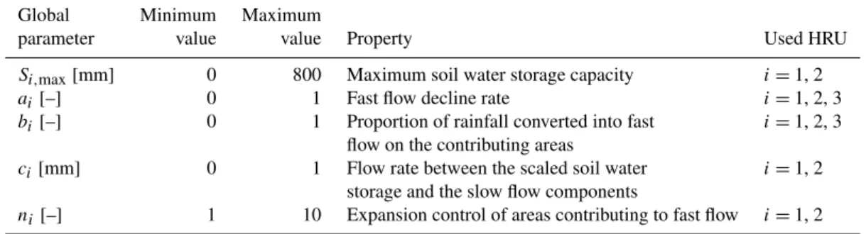
For each time step, we constructed maps showing for each pixel the fraction of accepted parameter sets (out of a total of 724 accepted sets for Version 2 and 606 accepted sets for Version 3) that resulted in fast flow in that pixel at the re-spective time. These maps give a picture of the uncertainty in the prediction of fast flow at the specific time across the catchment for the respective model version. For simplicity, we refer to the fraction of accepted parameter sets predicting fast flow as “risks” of fast flow. This measure reflects how sensitive the fast flow prediction is towards changes of the parameter sets. We introduce four classes and denote values ranging between 0 and 0.2 a low risk, values between 0.2 and 0.5 a medium risk, values between 0.5 and 0.8 a high risk, and values between 0.8 and 1 a very high risk of fast flow.

(10)

16 % (Version 2) or even 21 % (Version 3) of the agricultural area was very high risk area. Also the percentage of high and medium risk areas within the catchment increased dur-ing this event (Table 5). On the other hand, large fractions of the catchment were considered at low risk during the small event by both model versions (76 and 48 %, respectively). However, during the June event, model Version 3 predicted a low risk for only 13 % of the catchment, while this percent-age was higher (44 %) for model Version 2. Hence, based on the model results one cannot exclude the risk for DRP losses from a considerable fraction of the area.

The spatial patterns of predicted fast flow risk areas were very similar for model versions 2 and 3 (Table 5, Fig. 6). The major difference was that the medium risk was more preva-lent and the low risk class less frequent in Version 3 than in Version 2. This can be attributed to the lower overall runoff in Version 3 simulations, which led to higher soil moisture predictions and thus lower topographical threshold values.

3.2.2 Spatial predictions of DRP losses from soil

In the RRP model, the risk of P loss depends on the combi-nation of runoff risk and the presence of DRP at a given lo-cation. While manure is a DRP source that decreases rapidly after application and can be managed, soil DRP has much slower dynamics and is always present as a source (Kleinman et al., 2011a). Areas with high simulated DRP loads were mainly distributed along the stream network, or in flat areas with high soil P concentrations a bit farther away from the stream (Fig. 7). There was little difference between the two model versions regarding the area that is expected to con-tribute the most. The extent of the hatched area in Fig. 7 however was larger for Version 3 than for Version 2. The hatched area illustrates where less than 80 % of the simu-lations resulted in the same distribution of fast flow gen-eration and thus indicates where model predictions were fairly uncertain. Accounting for all model predictions, we calculated the average DRP load for each pixel. For 90 % of the agricultural area in the Stägbach catchment, the av-erage DRP load calculated over the whole simulation pe-riod was below 14.9 mg h−1pixel−1 for Version 2 and be-low 13.7 mg h−1pixel−1for Version 3. The remaining 10 % of the agricultural area delivered more than half of the to-tal load exported from agricultural land (Version 2: 52 %, Version 3: 54 %). Neglecting winter months, the estimated yearly DRP loads from 10 % of the agricultural area averaged 3.4 kg ha−1(Version 2) and 3.1 kg ha−1(Version 3). During the large runoff event in June 2010, much higher loads per hour were simulated. Again, 10 % of the agricultural area de-livered more than 50 % of the DRP load from the total agri-cultural area. The estimated load per hectare for 10 % of the area averaged 24 g ha−1h−1 (Version 2) and 29 g ha−1h−1 (Version 3) during this event.

Table 5.Spatial extent of risk classes in the Stägbach catchment for different model versions and two runoff events in 2010 – relative to the total agricultural area in %.

Risk classes Low Medium High Very high Risk values 0 to 0.2 0.2 to 0.5 0.5 to 0.8 0.8 to 1

Version 2

small event in May 76 12 5 7

large event in June 44 23 17 16

Version 3

small event in May 48 41 4 7

large event in June 13 50 16 21

A B

Fig. 6.Risk maps for the large event of June 2010 in the Stägbach catchment, obtained with model versions 2 (left) and 3 (right). Grey shading denotes forested and urban areas

3.3 Spatial model performance and field measurements

3.3.1 Test of model assumptions

(11)

A

A B

Fig. 7.Simulated distribution of DRP loads in the Stägbach catch-ment during the large event in June 2010 obtained by averaging over all Monte Carlo simulations. Red color shows the area (10 % of the total agricultural area) where according to the simulations more than 50 % of the total DRP loss occurred. Areas for which less than 80 % of the simulations resulted in the same distribution of fast flow generation are hatched. Grey shading denotes forested and urban areas.

well-drained HRU according to the classification used in Ver-sion 2. Thus, the results suggest that soil moisture was more closely related to topographic index than to soil drainage cat-egory.

3.3.2 Model predictions and soil moisture measurements

Figure 8 furthermore shows that the predicted risk of fast flow was closely related to measured soil water saturation, confirming the validity of the hydrological simulations pre-sented before. At the two stations with highλvalues (S2, S3), the predicted risk of fast flow strongly increased when soil moisture approached full saturation, while there was gener-ally a very low risk of fast flow with comparatively little re-sponse to variations in soil moisture at the two stations with lowλvalues (S1, S4). Version 3 consistently predicted higher risks of fast flow than Version 2, in line with the results pre-sented in Sect. 3.2.1.

3.3.3 Model predictions, OFD and groundwater measurements

The model predictions of fast flow risks were also in rea-sonable agreement with runoff data recorded by the OFD (Fig. 8). Surface runoff occurred at sites S2 and S3 when both model versions predicted a risk of fast flow above 0.75. No runoff was collected when the predicted risk was below 0.5. On the other hand, runoff was never observed at station S1, for which the predicted risk values were always below 0.05 for model Version 2 and 0.225 for model Version 3. Some

0

0.5

1Risk and OFD

S1

W

ater Satur

ation of the Soil

median TDR − 30 cm median TDR − 10 cm risk to generate fast flow − version2 risk to generate fast flow − version3 Runoff detected

0

0.5

1

0

0.5

1 Risk and OFD

S2

W

ater Satur

ation of the Soil

0

0.5

1

0

0.5

1Risk and OFD

S3

W

ater Satur

ation of the Soil

0

0.5

1

0

0.5

1 Risk and OFD

S4

W

ater Satur

ation of the Soil

0

0.5

1

Fig. 8.Comparison of soil moisture measurements, runoff measure-ments (with overland flow detectors, OFDs) and model predictions of fast flow risks at the four permanent soil moisture measurement stations in the Stägbach catchment for the year 2010.

over-prediction of runoff risks may be due to the fact that OFDs only collect surface runoff, whereas predicted fast flow also includes preferential flow in the RRP model. This may in particular have been the case at station S7, which was one of the six other measurement stations that were not perma-nently operated. For this location both model versions often predicted high fast flow risks, sometimes even in all simula-tions, but runoff was collected only once with the installed OFD. This station was located close to a brook where a large amount of the simulated runoff may actually have been due to subsurface flow. In contrast to stations S1, S2, S3 and S7, the risk of runoff from station S4 was underestimated. Sur-face runoff was collected at S4 during the large event in June, while model Version 2 predicted fast flow only in 6 % of the simulations. Similarly, no elevated risk was predicted for the event at the end of July, when 10 mL of runoff were col-lected (Fig. 8). Using model Version 3 substantially higher risks of fast flow were predicted for S4 than by Version 2, but even for the extreme event in June the predicted risk still did not exceed a value of 0.3. Similar under-predictions of runoff risks were also obtained for one event at sites S5, S8 and S10, where runoff was collected by the OFD, while the predicted risks remained below 0.1 for model Version 2 and below 0.3 for model Version 3. At two of the three locations, infiltration excess runoff or runoff from a street farther up-slope may have had some influence.