Submitted22 August 2016
Accepted 12 October 2016
Published8 November 2016
Corresponding author
Bert O. Baumgaertner, [email protected]
Academic editor
Tomas Perez-Acle
Additional Information and Declarations can be found on page 17
DOI10.7717/peerj.2678 Copyright
2016 Nardin et al.
Distributed under
Creative Commons CC-BY 4.0 OPEN ACCESS
Planning horizon affects prophylactic
decision-making and epidemic dynamics
Luis G. Nardin1,*, Craig R. Miller1,2,3,*, Benjamin J. Ridenhour1,2, Stephen M. Krone1,3, Paul Joyce1,3,†and Bert O. Baumgaertner1,4
1Center for Modeling Complex Interactions, University of Idaho, Moscow, ID, United States 2Department of Biological Sciences, University of Idaho, Moscow, ID, United States 3Department of Mathematics, University of Idaho, Moscow, ID, United States
4Department of Politics and Philosophy, University of Idaho, Moscow, ID, United States
*These authors contributed equally to this work.
†Deceased.
ABSTRACT
The spread of infectious diseases can be impacted by human behavior, and behavioral decisions often depend implicitly on a planning horizon—the time in the future over which options are weighed. We investigate the effects of planning horizons on epidemic dynamics. We developed an epidemiological agent-based model (along with an ODE analog) to explore the decision-making of self-interested individuals on adopting prophylactic behavior. The decision-making process incorporates prophylaxis efficacy and disease prevalence with the individuals’ payoffs and planning horizon. Our results show that for short and long planning horizons individuals do not consider engaging in prophylactic behavior. In contrast, individuals adopt prophylactic behavior when considering intermediate planning horizons. Such adoption, however, is not always monotonically associated with the prevalence of the disease, depending on the perceived protection efficacy and the disease parameters. Adoption of prophylactic behavior reduces the epidemic peak size while prolonging the epidemic and potentially generates secondary waves of infection. These effects can be made stronger by increasing the behavioral decision frequency or distorting an individual’s perceived risk of infection.
SubjectsMathematical Biology, Epidemiology, Infectious Diseases, Public Health, Computational Science
Keywords Human behavior, Behavioral epidemiology, ODE, Infectious diseases, Prophylaxis, Agent-based modeling
INTRODUCTION
Human behavior plays a significant role in the dynamics of infectious disease (Ferguson,
2007;Funk, Salathé & Jansen, 2010). However, the inclusion of behavior in epidemiological
modeling introduces numerous complications and involves fields of research outside the biological sciences, including psychology, philosophy, sociology, and economics. Areas of research that incorporate human behavior into epidemiological models are loosely referred to associal epidemiology,behavioral epidemiology, oreconomic epidemiology (Manfredi &
D’Onofrio, 2013;Philipson, 2000). We use the term ‘behavioral epidemiology’ to broadly
behavioral epidemiology is to understand how social and behavioral factors affect the dynamics of infectious disease epidemics. This goal is usually accomplished by coupling models of social behavior and decision making with biological models of contagion (Perrings et al., 2014;Funk, Salathé & Jansen, 2010).
Many social and behavioral aspects can be incorporated into a model of infectious disease. One example is the effect of either awareness or fear spreading through a population (Funk et al., 2009;Epstein et al., 2008). In these types of models, the spread of beliefs or information is treated as a contagion much like an infectious disease, though the network for the spread of information may differ from the biological network (Bauch & Galvani, 2013). Other models focus on how individuals adapt their behavior by weighting the risk of infection with the cost of social distancing
(Fenichel et al., 2011;Reluga, 2010) or other disincentives (Auld, 2003). Still others model
public health interventions (e.g., isolation, vaccination, surveillance, etc.) and individual responses to them (Del Valle et al., 2005). Many of these models sit at the population level, incorporating the effects of social factors and abstracting away details about the individuals themselves.
The SPIR model (Susceptible,Prophylactic,Infectious,Recovered) developed here, in contrast, is an epidemiological model that couples individual behavioral decisions with an extension of the SIR model (Kermack & McKendrick, 1927). In this model agents that are vulnerable to infection may be in one of two states,susceptible orprophylactic, which is determined by their behavior. Agents in the susceptible state engage in the status quo behavior while agents in the prophylactic state employ preventative behaviors that reduce their chance of infection. We use a rational choice model to represent individual behavioral decisions, where individuals select the largest utility between engaging in prophylactic behavior (e.g., hand-washing or wearing a face mask) or non-prophylactic behavior (akin to the status quo). We also allow for the fact that individuals may not perceive the risk of getting infected accurately, but rather receive distorted information, for example, through the media.
We use the SPIR model to understand how an individual’s planning horizon—the time in the future over which individuals calculate their utilities to make a behavioral decision—affects behavioral change and how that, in turn, influences the dynamics of an epidemic.
S
P
I
R
i
b
s
i
b
s
g
Behavioral Decision
Model
d
(
W
(
i
))
d
(1 ‑
W
(
i
))
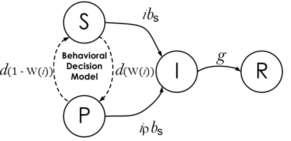
Figure 1 State-transition diagram of agents in the Disease Dynamics Model.S, P, I, and R represent the four epidemiological states an agent can be in: Susceptible, Prophylactic, Infectious, and Recovered, respectively. The parameters over the transitions connecting the states represent the probability per time step that agents in one state move to an adjacent state:iis the proportion of infectious agents in the pop-ulation;bSandbPare the respective probabilities that an agent in state S or P, encountering an infectious
agent I, becomes infected;gis the recovery probability;ρis the reduction in the transmission probability when an agent adopts prophylactic behavior that linearly relatesbSandbP, i.e.,bP=ρbS;dis the
behav-ioral decision making probability; and W(i) is an indicator function returning value 1 when the utility of being prophylactic is greater than the utility of being susceptible and 0 otherwise (see details in Behavioral Decision Model).
METHODS
The SPIR modelThe SPIR model couples two sub-models: one, theDisease Dynamics Model, reproducing the dynamics of the infectious disease, and another, the Behavioral Decision Model, that determines how agents in the disease dynamics model make the decision to engage in prophylactic or non-prophylactic behavior.
Disease dynamics model
The disease dynamics model reproduces the dynamics of the infectious disease in a constant population ofNagents. Each agent can be in one of four states: Susceptible (S), Prophylactic (P), Infectious (I), or Recovered (R). The difference between agents in states S and P is that the former engage in non-prophylactic behavior and do not implement any measure to prevent infection, while the latter adopt prophylactic behavior which decreases their probability of being infected (e.g., wearing a mask, washing hands, etc.). The adoption of prophylactic behavior, however, imposes costs on individuals that may prevent them from engaging in such behavior. In Western countries, for example, wearing a mask, other than uncomfortable, may signal a lack of trust in others or an unhealthy state, thus reducing social contacts. Agents in the infectious state I are infected and infective, while those in the recovered state R are immune to and do not transmit disease. The transition between states is captured with the state-transition diagram shown inFig. 1. For reference, all the parameters and variables in the SPIR model are listed and defined inTable 1.
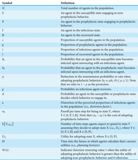
Table 1 Parameters and state variables of the SPIR model.
Symbol Definition
N Total number of agents in the population.
S An agent in the susceptible state engaging in non-prophylactic behavior.
P An agent in the prophylactic state engaging in prophylactic behavior.
I An agent in the infectious state.
R An agent in the recovered state.
s Proportion of susceptible agents in the population.
p Proportion of prophylactic agents in the population.
i Proportion of infectious agents in the population.
r Proportion of recovered agents in the population.
bS Probability that an agent in the susceptible state becomes
infected upon interacting with an infectious agent.
bP Probability that an agent in the prophylactic state becomes
infected upon interacting with an infectious agent. ρ Reduction in the transmission probability or rate when
adopting prophylactic behavior:bP=ρbS(0≤ρ≤1). Note
that we refer to 1−ρas theprotection.
g Probability an infectious agent recovers.
d Probability an agent in the susceptible or prophylactic state decides which behavior to engage in.
κ Distortion of the perceived proportion of infectious agents in the population (i.e.,distortion factor).
uY Payoff per time step for being in state Y, where
Y∈ {S,P,I,R}. Note that (uS−uP) is the cost of adopting
prophylactic behavior. E
TY|DX
Number of time steps agents expect to spend in state Y assuming they decide to adopt state X (i.e., DX), where Y∈ {S,P,I,R}and X∈ {S,P}.
UX Utility for adopting state X, where X∈ {S,P}.
H Time into the future at which agents calculate their current utilities (i.e.,planning horizon).
W(i) Indicator function returning value 1 when the utility of adopting prophylactic behavior is greater than the utility of adopting non-prophylactic behavior and 0 otherwise.
Table 2 Disease parameters in rates and probabilities.
Rate parameter Probability parameter Description Probability to rate conversion
β bS Transmission β= −ln(1−bS)
γ g Recovery γ= −ln 1−g
δ d Decision δ= −ln(1−d)
agentsirepresents the probability that an agent is paired with an infectious agent and the per time step probability of an agent in state S or P being infected isibSoribP, respectively. In addition to interacting, susceptible and prophylactic agents have probabilitydper time step of making a behavioral decision to engage in prophylactic or non-prophylactic behavior. The agents’ behavioral decision is reflected in the indicator function W(i) (see details in Behavior Decision Model), and they engage in the prophylactic behavior when W(i)=1 (i.e., adopt state P) and the non-prophylactic behavior when W(i)=0 (i.e., adopt state S). Infectious agents have probabilityg per time step of recovering. We implemented an agent-based version of the disease dynamics model using the Gillespie algorithm (Gillespie, 1976) (source code available inSupplemental Information 1).
Our agent-based model (ABM) is a useful tool for exploring the aggregated effects of individual decision making, including scenarios where populations are heterogeneous (e.g., some individuals may be more risk-averse than others). A drawback of this model is that it requires simulations that can be computationally intensive. The stochasticity of the ABM further exacerbates the computational burden when mean results are desired. If, however, we assume that the population is well-mixed, the dynamics can be generated using a system of ODEs (see Sec. S7 inSupplemental Information 1for a comparison):
ds
dt = −βsi−δsW(i)+δp(1−W(i)) (1a)
dp
dt = −ρβpi+δsW(i)−δp(1−W(i)) (1b)
di
dt =βsi+ρβpi−γi (1c)
dr
dt =γi (1d)
wheres,p,i, andrare the proportion of susceptible, prophylactic, infectious, and recovered agents in the population. The parameters β,γ, andδ are transmission, recovery, and decision rates, whose equivalent probabilities are, respectively, transmission (bS), recovery (g), and decision (d) (Table 2). The parameterρrefers to the reduction in transmission rate when adopting prophylactic behavior. We convert between rates and probabilities using equationsx= −ln 1−yandy=1−e−x, wherexandy are rate and probability values respectively (Fleurence & Hollenbeak, 2007). One unit of continuous time in the ODE model corresponds toN time steps in the ABM.
Behavioral decision model
any model that enables agents to decide whether or not to engage in prophylactic behavior. Our decision model is a rational choice model that assumes agents are self-interested and rational; thus they adopt the behavior with the largest utility over the planning horizon, H. Note that the planning horizon is a construct used to calculate utilities and it does not affect the time until an agent has an opportunity to make another decision within the disease dynamics model.
The planning horizon is the time in the future over which agents calculate their utilities. In order for the agent to make these calculations, we make the following assumptions about agents tasked with making a decision; (1) Agents have identical and complete knowledge of the relevant disease parameters,bS,bP, andg. (2) Prophylactic behavior has the same pro-tection efficacy,ρ, for all agents; (3) Agents believe the current prevalence of the disease isi (in the case of no distortion—see below); (4) Agents assume thatiwill remain at its current value during the next H time steps; (5) Agents compute expected waiting times based on a censored geometric distribution. Specifically, they believe that they will spend the amount of timeTXin state X∈ {S,P}, where the timeTXhas a geometric distribution with parameteribX, censored at the planning horizon H. When their time in X is over, agents know they will move to state I where the amount of time they expect to spend in state I has a geometric distribution with parameterg censored at the time remaining, H−TX. When their time in state I is over, they know they will move to state R where they will remain until time H. (6) Agents know the per time step payoff for each stateuY, where Y∈ {S,P,I,R}, and all agents are assumed to have the same set of payoff values. (7) Agents calculate the sum of the utility from now until time H under the two possible behavioral decisions (DSor DP).
Perfect knowledge of i.To calculate the utilities when they have perfect knowledge ofi,
agents use the length of time they expect to spend in each state. We begin by deriving the expected time in state X, where X∈ {S,P}, and then we use this result to derive the expected time in I and, finally, R. The expected time in state I is conditioned onTXbecause agents are rational and they average the time they expect to spend on state I over all possible hypothetical combinations involving X and I up to H. To simplify notation, it is helpful to first define the force of infection for state X, fX:fS=ibSandfP=iρbS. For the agent considering hypothetical futures, the planning horizon serves to censor all waiting times greater than H, giving them value H. This leads to the following probability mass function for the time spent in state X should they decide on behavior X (denotedTX|DX),
Pr TX|DX=t
=
fX 1−fXt, 0≤t<H
1−fX H
, t=H
0, otherwise.
(2)
The expected time spent in state X can be expressed as
E TX|DX
=
H X
t=0
tfX 1−fX
t
+H 1−fX H
which simplifies to the desired expectation,
E TX|DX
= 1 fX −1
1− 1−fX
H
. (4)
Notice thatf1 X−1
is the expected time to remain in state X before moving to state I for an uncensored geometric with minimum value of zero, while the second parenthetical term rescales the expectation to the interval[1,H].
Next, we derive the expected time spent in I by conditioning onTX|DX.
E TI|DX
=E
E
TI|DX|TX|DX
=E
1
g−1
1− 1−gH−TX|DX
. (5)
After considerable algebra (see Sec. S3 in Supplemental Information 1), we get the expectation,
E TI|DX
=
1
g−1
1
g−1 1− 1−g
H
−
1
fX−1 1− 1−fX
H
1 g−1
−
1 fX−1
. (6)
Again, the expectation of the uncensored geometric is
1 g−1
. The second parenthetical term compresses the expected time into the interval between ETX|DX
and H. Notice that
Eq. (6)is defined only so long asfX6=g. WhenfX=g, we instead have
ETI|DX
=
1
g−1
1− 1−gH−H 1−gH+1. (7)
Finally, the agent calculates the expected time in state R by subtracting the expectations for X and I from H,
E[TR|DX] =H−E
TX|DX
−E TI|DX
. (8)
Notice that for each of the expected waiting times calculated in Eqs. (4),(6)and(7), as H goes to infinity, the rescaling terms go to one so that the equations yield the familiar expected values for the uncensored geometrics.
Having calculated these expected waiting times, the agent then calculates the utility for the two possible behaviors using,
US=uSETS|DS
+uIETI|DS
+uRETR|DS
(9)
and
UP=uPE
TP|DP
+uIE
TI|DP
+uRE
TR|DP
. (10)
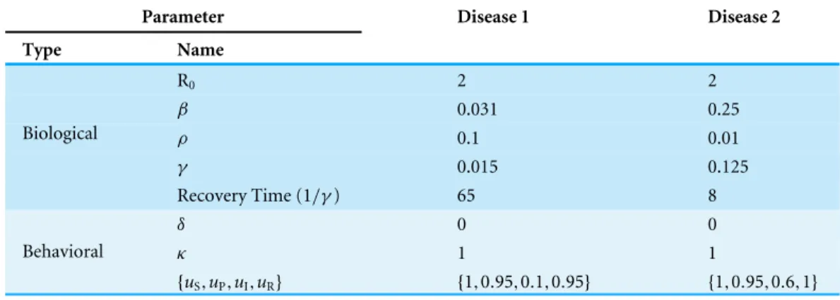
Table 3 Input parameters for two hypothetical contrasting diseases.
Parameter Disease 1 Disease 2
Type Name
R0 2 2
β 0.031 0.25
ρ 0.1 0.01
γ 0.015 0.125
Biological
Recovery Time (1/γ) 65 8
δ 0 0
κ 1 1
Behavioral
{uS,uP,uI,uR} {1,0.95,0.1,0.95} {1,0.95,0.6,1}
during H. Thus, E TS|DP
and E
TP|DS
are both zero. To be clear, this constraint pertains only to calculating utilities; agents are not constrained in how many times they actually switch states during the epidemic.
Because decisions reflect the largest utility and because the population is homogeneous, the behavioral decision can be expressed as the indicator function W(i)defined by
W(i)= (
1 for US<UP
0 otherwise (11)
Distorting knowledge of i. Recall that assumption (3) that underlies the behavioral decision
model is that agents know the prevalence of the disease accurately. We relax this assumption to investigate how distorting this information affects the epidemic dynamics. To achieve this, we replaceiwithi1κ in the calculation of utilities whereκ serves as adistortion factor. Whenκ=1,iis not distorted; whenκ >1, the agent perceivesito be above its real value and whenκ <1 the opposite is true. To implement this distortion, we redefinefXin the expected waiting time equations (i.e.,Eqs. (3)–(7)) withfX=i
1
κbSwhen X=S and
fX=i
1
κρbSwhen X=P.
RESULTS AND ANALYSIS
The SPIR model can be applied to a diverse range of infectious disease epidemics and how they might be impacted by human behavior. To illustrate specific characteristics of the model, however, we focus here on two contrasting diseases characterized by their severity, recovery time, and harm: Disease 1is acute, has a long recovery time, and may cause chronic harm, andDisease 2is mild, has a short recovery time, and causes no lasting harm.
Table 3shows the biological and behavioral parameter values used to generate the results discussed next, unless stated otherwise. Note that the results were generated using the ODE model that is more computationally efficient than the ABM, but generates the same results (see Sec. S7 inSupplemental Information 1for a comparison).
Behavioral decision analysis
A
0% 50% 100%
Utility
B
0% 50% 100%
% Infectious (i)
C
0% 50% 100%
Susceptible Prophylactic
30% 90%
A B
C
D
0% 25% 50% 75% 100%
0 100 200 300 400
Planning Horizon (H)
% Protection
0% 25% 50% 75% 100%
% Infectious (i)
Figure 2 Heat map of switching points for Disease 1.(A) Situation in which non-prophylactic behavior is always more advantageous than prophylactic behavior regardless of the proportion of infectious agents. (B) Situation in which above a certain proportion of infectious agents (indicated by the vertical dotted line), the prophylactic behavior is more advantageous than non-prophylactic behavior. (C) Situation in which prophylactic behavior is more advantageous whenever the proportion of infectious agents is within a range of values represented by the two vertical dotted lines and less advantageous otherwise. (D) Propor-tion of infectious agents above which prophylactic behavior is more advantageous than non-prophylactic behavior given the percentage of protection (% Protection) obtained for adopting prophylactic behavior (1−ρ)×100 (y-axis) and the planning horizon H (x-axis). The three regions in (D) represent the sit-uations shown in (A), (B), and (C). In regionA, agents never adopt prophylactic behavior. In regionB, agents adopt prophylactic behavior above the reported proportion of infectious agents. In regionC, agents adopt prophylactic behavior only if the proportion of infected agents is between the proportion of infec-tious agents represented by the color gradient and the proportion represented by the contour lines.
of disease prevalence above which agents would switch behavior, i.e., aswitching point. A switching point is defined as the proportion of infectious agents beyond which it would be advantageous for an agent to switch from non-prophylactic to prophylactic behavior or vice-versa. We can visualize switching points by plotting the expected utility for the susceptible and prophylactic states as a function of the proportion of infectious agents. A switching point is where the expected utilities cross, if they cross.Figure 2Aillustrates the situation in which the utilities do not cross, thus there is no switching point.Figure 2B
illustrates the situation in which there is a single switching point; below the switching point the susceptible state has the higher utility, whereas above that point the prophylactic state has the higher utility.Figure 2Cshows the situation in which the utilities cross twice, thus there are two switching points; between the switching points the prophylactic state has the higher utility, whereas the susceptible state has higher utility on the margins.
S
I
R
A
0% 25% 50% 75% 100%
0 100 200 300
Expected % of H
P I
R
B
0% 25% 50% 75% 100%
0 100 200 300
Planning Horizon (H)
Figure 3 Expected proportion of the planning horizon spent in each state.(A) Proportion of the plan-ning horizon agents expect to spend in each state if they decide to adopt state S. (B) Proportion of the planning horizon agents expect to spend in each state if they decide to adopt state P. For short planning horizons, the largest proportion of time is expected to be spent in the susceptible or prophylactic states. Increasing the planning horizon increases the proportion of H that an agent expects to spend in the recov-ered state.
A corresponds to the situation in which agents never engage in prophylactic behavior because the utility of being in the susceptible state is never less than the prophylactic state regardless of disease prevalence (Fig. 2A). This situation occurs for low protection efficacy or short planning horizons. In the case of low protection efficacy, agents do not have an incentive to adopt prophylactic behavior because they expect to get infected regardless of their behavior. Thus, their best strategy is to become infected and then recover in order to collect the recovered payoff as quickly as possible (i.e., ‘‘get it over with’’). In the case of short planning horizons, the relative contributions of the expected times of being in the susceptible or prophylactic state dominate the utility calculations, as shown inFig. 3. The figure illustrates how, when the planning horizon is short, the expected percentage of time spent in the susceptible or prophylactic states are much greater than the expected percentage of time spent in the infectious or recovered state. Given that the susceptible payoff is greater than the prophylactic payoff, agents never adopt prophylactic behavior. The figure also shows how increasing the planning horizon changes the distribution of time spent in each state, which reduces the influence of the difference between the susceptible and prophylactic payoffs on behavioral decision.
A 0% 25% 50% 75% 100%
0 100 200 300 400
% Protection
uS = uR > uP B
0% 25% 50% 75% 100%
0 100 200 300 400
uS > uR > uP C
0% 25% 50% 75% 100%
0 100 200 300 400
uS > uR = uP D
0% 25% 50% 75% 100%
0 100 200 300 400
0% 25% 50% 75% 100%
% Infectious (i)
uS > uP > uR
E 0% 25% 50% 75% 100%
0 100 200 300 400
% Protection
uS = uR > uP F
0% 25% 50% 75% 100%
0 100 200 300 400
uS > uR > uP G
0% 25% 50% 75% 100%
0 100 200 300 400
uS > uR = uP H
0% 25% 50% 75% 100%
0 100 200 300 400
0% 25% 50% 75% 100%
% Infectious (i)
uS > uP > uR
Planning Horizon (H)
Disease 2 Disease 1
Figure 4 Heat maps of switching points under qualitatively different payoff relationships for Disease 1 and Disease 2.The heat maps in (A)–(D) correspond to Disease 1 and the heat maps in (E)–(H) corre-spond to Disease 2. In (A) and (E) the payoff of being susceptible and recovered are equal, which means that agents recover completely from the disease after infection. In (B) and (F), the recovered payoff is lower than the susceptible payoff, but still greater than the prophylactic payoff meaning that being recov-ered is preferable to than being in the prophylactic state. In (C) and (G), the payoff for the prophylactic and recovered states are exactly equal. In (D) and (G), the disease is permanently debilitating such that the payoff of the recovered state is less than the prophylactic state. The heat maps of behavioral change assume the following payoffs foruS,uP,uI,uR. (A):{1, 0.95, 0.1, 1}, (B):{1, 0.95, 0.1, 0.97}, (C):{1, 0.95, 0.1, 0.95},
(D):{1, 0.95, 0.1, 0.9}, (E):{1, 0.95, 0.6, 1}, (F):{1, 0.95, 0.6, 0.97}, (G):{1, 0.95, 0.1, 0.95}, and (H):{1, 0.95, 0.1, 0.9}. The % Protection corresponds to the percentage of protection obtained for adopting prophylac-tic behavior, (1−ρ)×100.
the adoption of prophylactic behavior is not always monotonically associated with the prevalence of the disease.
The utility calculations that agents use to decide whether to adopt a behavior are complex (seeEqs. (9)and(10)); an exhaustive exploration of the parameter space is not undertaken here. We instead investigate several paradigm cases related to the payoff ordering. We assume that the payoff for the infectious state (uI) relies upon biological parameters of the disease and always corresponds to the lowest payoff, thus we need only consider the relationship between the other three payoffs. In particular, we are interested in looking at situations where the recovery payoff ranges from complete recovery (case 1) to less than the prophylactic state (case 4).
Case 1: uS=uR>uP>uI,
Case 2: uS>uR>uP>uI,
Case 3: uS>uR=uP>uI, and
Case 4: uS>uP>uR>uI.
Because our model consists of a constant population ofN agents (i.e., no mortality), cases in whichuS>uRrepresent situations where an individual suffers chronic harm from the disease.
disease recovery time for Disease 1 is large (Recovery Time=65), but small for Disease 2 (Recovery Time=8). Consequently, an agent expects to spend more time in the recovered state when considering Disease 2 than Disease 1. When weighting these expected times with different payoffs for calculating the utilities, there will be less variation in Disease 1 compared with Disease 2.
The effects of progressively reducing the recovered payoff are more evident for Disease 2. Reducing the recovered payoff means that lower levels of prevalence will be sufficient for agents to change their behavior. In the case of equal value for recovered and susceptible payoffs, agents consider changing behavior only in narrow parameter range of protection efficacy and planning horizon values (Fig. 4E). Progressively reducing the recovered payoff, i.e., moving from case 1 (Fig. 4E) to case 4 (Fig. 4H), the range of parameter values that induce agents to change their behavior expands (i.e., there are large areas of the parameter space in which the agents would consider changing behavior) and the disease prevalence necessary for such change to occur decreases (i.e., gradual change of the color towards blue).
In addition to this numerical analysis, we have also obtained analytical results for case 2 (payoff ordering uS>uR>uP>uI) that are available in Sec. S4Supplemental Information 1.
Epidemic dynamics
We turn now to understand how the above conditions for behavioral change may influence epidemic dynamics. Here we are particularly interested in analyzing the effects of the planning horizon H and the decision frequencyδon the dynamics of Disease 1 and Disease 2. Because we assume that the interactions among the population are well-mixed, we execute the simulations using the ODE model for a population of 100,000 agents (initially 99,900 agents in the susceptible state and 100 in the infectious state) with a decision frequency ofδ=0.01.
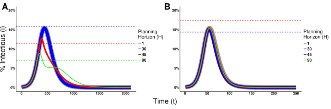
Figure 5shows the effects of different planning horizons on the epidemic dynamics for both Disease 1 (Fig. 5A) and Disease 2 (Fig. 5B). For short planning horizons (i.e., H=1), agents do not ever consider changing behavior in either disease. This corresponds to the situation in RegionAinFig. 2Ain which being prophylactic is never worth the cost, hence the epidemic dynamics are not affected. Similarly, in the cases of H=30 for Disease 1 and H=45 for Disease 2, we notice that neither of the two epidemic dynamics change. The dynamics are not affected because the disease prevalence does not reach the switching point (the switching points are indicated by the dashed lines inFig. 5).
In the cases of H=45 and 90 for Disease 1 and H=30 for Disease 2, however, agents change behavior and thereby affect epidemic dynamics. For Disease 1, the effect is characterized by the decrease on the epidemic peak size and a prolonged duration of the epidemic. Although the dynamics of Disease 2 are also affected, the effect is small because a lower portion of the population crosses the switching point.
A
0% 5% 10% 15% 20%
0 500 1000 1500 2000
% Inf
ectious (i)
Planning Horizon (H)
1 30 45 90
B
0% 5% 10% 15% 20%
0 50 100 150 200 250
Planning Horizon (H)
1 30 45 90
Time (t)
Figure 5 Effects of the Planning Horizon on the epidemic dynamics.The solid lines represent the pro-portion of infectious agents in the population over time. The line thickness is not meaningful; rather, it is used to facilitate the visualization due to the fact that the dynamics overlap each other. The dashed lines represent the switching point associated to the planning horizon reported with the same color in the leg-end. Missing dashed lines indicate that no switching point exists for that planning horizon. (A) Epidemic dynamics for Disease 1 with payoffs {1, 0.95, 0.1, 0.95} andρ=0.1. (B) Epidemic dynamics for Disease 2 with payoffs {1, 0.95, 0.6, 1} andρ=0.01. Both dynamics consider decision frequencyδ=0.01 for plan-ning horizons 1, 30, 45, and 90.
2. This means that agents willingly assume the risk of getting infected and then recover, which is intuitive given the short recovery time and mild severity of the disease.
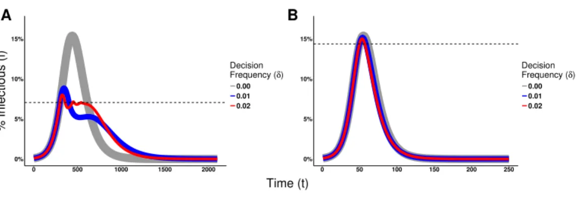
To assess the effect of the frequency that agents make behavioral decisions on the epidemic dynamics, we fix the value of the planning horizon for Disease 1 (H=90) and Disease 2 (H=30), and vary the decision rate. Figure 6shows the effects of different decision frequencies on the epidemic dynamics. This figure illustrates how increasing the decision frequency reduces the epidemic peak size while prolonging the epidemic. It additionally may generate multiple waves of infection for Disease 1. These waves are generated because raising the decision frequency means individuals react faster to an increase in prevalence and adopt the prophylactic behavior. This bends the trajectory of disease incidence downward, but the reduction in prevalence causes the pendulum to swing back and individuals return back to their non-prophylactic behavior, thus creating an environment for the resurgence of the epidemic.
Risk perception
Empirical evidence shows that humans change behavior and adopt costly preventative measures, even if disease prevalence is low. This is especially true for harmful diseases with severe consequences to those being infected, such as Ebola or the Severe Acute Respiratory Syndrome (SARS). For example, despite the low level of recorded cases during the 2003 SARS outbreak in China (approximately 5,327 cases), people in the city of Guangzhou avoided going outside or wore masks when outside (World Health Organization, 2003;Tai
& Sun, 2007). Combined with the severity of the disease, other factors like misinformation
or excess media coverage may distort the perception of disease prevalence (i.e., risk perception), making individuals respond unexpectedly to an epidemic.
A
0% 5% 10% 15%
0 500 1000 1500 2000
% Inf
ectious (i)
Decision Frequency (δ)
0.00 0.01 0.02
B
0% 5% 10% 15%
0 50 100 150 200 250
Decision Frequency (δ)
0.00 0.01 0.02
Time (t)
Figure 6 Effects of the Decision Frequency on the epidemic dynamics.The solid lines represent the pro-portion of infectious agents in the population over time. The line thickness is not meaningful; rather, it is used to facilitate the visualization due to the fact that the dynamics overlap each other. The dashed lines represent the switching point of H=90 for Disease 1 and H=30 for Disease 2. (A) Epidemic dynamics for Disease 1 with payoffs {1, 0.95, 0.1, 0.95} andρ=0.1. (B) Epidemic dynamics for Disease 2 with payoffs {1, 0.95, 0.6, 1} andρ=0.01.
Here our focus is slightly different. We are interested in understanding the effects that such distorted perception has on the epidemic dynamics. Thus in our model, we have incorporated adistortion factorκthat alters the agents’ perception about disease prevalence used in calculating their utilities. Forκ=1, agents have the true perception of the disease prevalence; forκ >1, the perceived disease prevalence is inflated andκreflects an increase in the risk perception of being infected; for κ <1, the perceived disease prevalence is reduced below its true value.
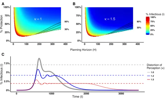
Distorting the perception of a disease prevalence can lead to changes in the decision making process, and consequently on epidemic dynamics, as illustrated inFig. 7for Disease 1 (seeFig. S2for Disease 2).Figure 7Ashows the switching point assuming agents know the real disease prevalence (κ=1). By distorting the perceived disease prevalence (κ=1.5), the real proportion of infectious agents necessary for agents to engage in prophylactic behavior is reduced as shown inFig. 7B. Hence, the distortion on disease prevalence makes agents engage in prophylactic behavior even when the chance of being infected is low. This affects the epidemic dynamics by reducing the epidemic peak size but prolonging the epidemic and generating multiple waves of infection as shown inFig. 7C.
DISCUSSION
Individuals acting in their own self-interest make behavioral decisions to reduce their likelihood of getting infected in response to an epidemic. We explore a decision making process that integrates the prophylaxis efficacy and the current disease prevalence with individuals’ payoffs and planning horizon to understand the conditions in which individuals adopt prophylactic behavior.
30% 90%
κ =1
A
0% 25% 50% 75% 100%
0 100 200 300 400
% Protection
30% 90%
κ =1.5
B
0% 25% 50% 75% 100%
0 100 200 300 400
0% 25% 50% 75% 100%
% Infectious (i)
Planning Horizon (H)
C
0% 2.5% 5% 7.5%
0 1000 2000 3000
Time (t)
% Inf
ectious (i)
Distortion of Perception (κ)
1.0 1.2 1.5
Figure 7 Heat maps of switching points and epidemic dynamics for Disease 1.(A) and (B) show the proportion of infectious agents above which the prophylactic behavior is more advantageous than the non-prophylactic behavior given the percentage of protection obtained for adopting the prophylactic be-havior (1−ρ)×100 and the planning horizon H. SeeFig. 2for more details on interpreting switching point heat maps. (A) No perception distortion:κ=1; (B) A distortion factorκ=1.5, which reduces the proportion of infectious agents above which the prophylactic behavior is more advantageous. (C) Epi-demic dynamics for different distortion factors show how increasingκreduces the epidemic peak size, prolongs the epidemic and generates secondary waves of infection.
situations, the epidemic dynamics remain unchanged because the individuals do not have an incentive to engage in prophylactic behavior even when the disease prevalence is high. For intermediate planning horizons, however, individuals adopt prophylactic behavior depending on the disease parameters and the prophylaxis efficacy. The effects on disease dynamics include a reduction in the epidemic peak size, but a prolonged epidemic.
The time scale of a planning horizon (i.e., what constitutes short, intermediate, and long), however, depends on the disease parameters. While the time scale for Disease 2 is on the order of days, for Disease 1 the time scale is on the order of months to years.
These results are consistent with the findings ofFenichel et al. (2011), who also concluded that behavioral change is sensitive to a planning horizon. The SPIR and Fenichel et al.
the same conclusion using different models further supports the claim that the planning horizon is a relevant decision making factor in understanding epidemic dynamics.
Although associated with the prevalence of disease, the adoption of prophylactic behavior is not always monotonically associated with it. Its adoption depends on the behavioral decision parameters. For severe diseases with long recovery times, e.g., Disease 1, the option of prophylactic behavior is less sensitive to changes in the payoffs (Figs. 4A–4D) compared to less severe diseases with shorter recovery times, e.g., Disease 2 (Figs. 4E–4H). This implies that understanding the payoffs related to each disease is critical to proposing effective public policies, especially because there is not a ‘‘one-size-fit-all’’ solution.
Another aspect to highlight is that the beneficial adoption of prophylactic behavior can be achieved through two different public policies: changing the risk perception or introducing incentives that reduce the difference between the susceptible and prophylactic payoffs (i.e., reduce the cost of adopting prophylactic behavior). One problem with increasing the risk perception is that if it is overdone, it leads, in some situations, to the opposite result to the one that is desired. Because individuals perceive their chance of getting the disease as highly probable, they prefer to ‘‘get it over with’’ and enjoy the benefits of being recovered. In contrast, the more the prophylaxis is incentivized the better the results, e.g., reduction of epidemic peak size.
Similar to our SPIR model, Perra et al. (2011)andDel Valle, Mniszewski & Hyman
(2013)also proposed an extension to the SIR model and included a new compartment
that reduces the transmission rate between the susceptible and infectious states. A clear distinction between these models and the SPIR model is that their agents do not take into account the costs associated with moving between the susceptible compartment and this new compartment. While inPerra et al. (2011)agents make the decision to move between compartments based on the disease prevalence, inDel Valle, Mniszewski & Hyman (2013)
constant transfer rates are defined to handle the transition.
ADDITIONAL INFORMATION AND DECLARATIONS
Funding
Research reported in this publication was supported by the National Institute Of General Medical Sciences of the National Institutes of Health under Award Number P20GM104420. This study was also supported by the Institute for Bioinformatics and Evolutionary Studies Computational Resources Core sponsored by the National Institutes of Health grant number P30GM103324 that provided us computer resources. This research made use of the resources of the High Performance Computing Center at Idaho National Laboratory, which is supported by the Office of Nuclear Energy of the US Department of Energy under Contract No. DE-AC07-05ID14517. The funders had no role in study design, data collection and analysis, decision to publish, or preparation of the manuscript.
Grant Disclosures
The following grant information was disclosed by the authors:
National Institute Of General Medical Sciences of the National Institutes of Health: P20GM104420.
National Institutes of Health: P30GM103324.
Office of Nuclear Energy of the US: DE-AC07-05ID14517.
Competing Interests
The authors declare there are no competing interests.
Author Contributions
• Luis G. Nardin conceived and designed the experiments, performed the experiments, analyzed the data, wrote the paper, prepared figures and/or tables, reviewed drafts of the paper.
• Craig R. Miller and Bert O. Baumgaertner conceived and designed the experiments, analyzed the data, wrote the paper, reviewed drafts of the paper.
• Benjamin J. Ridenhour wrote the paper, reviewed drafts of the paper, and provided mathematical analysis.
• Stephen M. Krone reviewed drafts of the paper, and provided mathematical analysis. • Paul Joyce provided mathematical analysis.
Data Availability
The following information was supplied regarding data availability: The raw data has been supplied asSupplemental Information 1.
Supplemental Information
REFERENCES
Auld MC. 2003.Choices, beliefs, and infectious disease dynamics.Journal of Health
Economics22(3):361–377DOI 10.1016/S0167-6296(02)00103-0.
Bandura A. 1986. Social foundations of thought and action : a social cognitive theory. Englewood Cliffs: Prentice-Hall.
Bauch CT, Galvani AP. 2013.Social factors in epidemiology.Science342(6154):47–49
DOI 10.1126/science.1244492.
Becker MH. 1974. The health belief model and personal health behavior.Health
Education Monographs, vol. 2. Thorofare: C.B. Slack.
Del Valle SY, Hethcote H, Hyman JM, Castillo-Chavez C. 2005.Effects of behavioral
changes in a smallpox attack model.Mathematical Biosciences195:228–251
DOI 10.1016/j.mbs.2005.03.006.
Del Valle SY, Mniszewski SM, Hyman JM. 2013. Modeling the impact of behavior
changes on the spread of pandemic influenza. New York: Springer, 59–77.
Epstein JM, Parker J, Cummings D, Hammond RA. 2008.Coupled contagion dynamics
of fear and disease: mathematical and computational explorations.PLoS ONE
3(12):e3955DOI 10.1371/journal.pone.0003955.
Fenichel EP, Castillo-Chavez C, Ceddia MG, Chowell G, Parra PAG, Hickling GJ, Hol-loway G, Horan R, Morin B, Perrings C, Springborn M, Velazquez L, Villalobos
C. 2011.Adaptive human behavior in epidemiological models.Proceedings of the
National Academy of Sciences of the United States of America108(15):6306–6311
DOI 10.1073/pnas.1011250108.
Ferguson N. 2007.Capturing human behaviour.Nature446(7137):733
DOI 10.1038/446733a.
Fleurence RL, Hollenbeak CS. 2007.Rates and probabilities in economic modelling.
Pharmacoeconomics25(1):3–6DOI 10.2165/00019053-200725010-00002.
Funk S, Bansal S, Bauch CT, Eames KTD, Edmunds WJ, Galvani AP, Klepac P. 2015. Nine challenges in incorporating the dynamics of behaviour in infectious diseases models.Epidemics10:21–25DOI 10.1016/j.epidem.2014.09.005.
Funk S, Gilard E, Watkins C, Jansen VAA. 2009.The spread of awareness and its impact
on epidemic outbreaks.Proceedings of the National Academy of Sciences of the United
States of America106(16):6872–6877DOI 10.1073/pnas.0810762106.
Funk S, Salathé M, Jansen VAA. 2010.Modelling the influence of human behaviour
on the spread of infectious diseases: A review.Journal of the Royal Society Interface 7:1247–1256DOI 10.1098/rsif.2010.0142.
Gillespie D T. 1976.A general method for numerically simulating the stochastic time evolution of coupled chemical reactions.Journal of Computational Physics
22(4):403–434DOI 10.1016/0021-9991(76)90041-3.
Kermack WO, McKendrick AG. 1927.A contribution to the mathematical theory of
epidemics.Proceedings of the Royal Society A: Mathematical, Physical and Engineering
Manfredi P, D’Onofrio A (eds.) 2013. Modeling the interplay between human behavior and the spread of infectious diseases. New York: Springer Science & Business Media.
Perra N, Balcan D, Gonćalves B, Vespignani A. 2011.Towards a characterization of
behavior-disease models.PLoS ONE6(8):e23084
DOI 10.1371/journal.pone.0023084.
Perrings C, Castillo-Chavez C, Chowell G, Daszak P, Fenichel EP, Finnoff D, Horan RD, Kilpatrick AM, Kinzig AP, Kuminoff NV, Levin S, Morin B, Smith KF,
Springborn M. 2014.Merging economics and epidemiology to improve the
prediction and management of infectious disease.EcoHealth11(4):464–475
DOI 10.1007/s10393-014-0963-6.
Philipson T. 2000. Economic epidemiology and infectious disease. In: Culyer AJ,
Newhouse JP, eds.Handbook of Health Economics, vol. 1, part B of Handbook of
Health Economics. Amsterdam: Elsevier, 1761–1799.
Poletti P, Ajelli M, Merler S. 2012.Risk perception and effectiveness of uncoordi-nated behavioral responses in an emerging epidemic.Mathematical Biosciences
238(2):80–89DOI 10.1016/j.mbs.2012.04.003.
Reluga TC. 2010.Game theory of social distancing in response to an epidemic.PLOS
Computational Biology6(5):e1000793DOI 10.1371/journal.pcbi.1000793.
Tai Z, Sun T. 2007.Media dependencies in a changing media environment: the
case of the 2003 SARS epidemic in China.New Media & Society9(6):987–1009
DOI 10.1177/1461444807082691.
World Health Organization. 2003.Consensus document on the epidemiology of