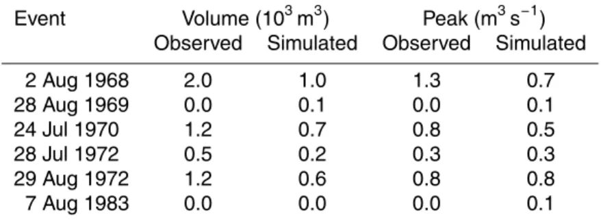
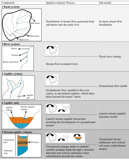
A channel transmission losses model for different dryland rivers
Texto
Imagem


Documentos relacionados
Eu sei o que vai dizer a seguir: «Por favor, dispense a Menina Quested do pagamento, para que os Ingleses possam dizer, Aqui está um nativo que efectivamente se comportou como
Maria II et les acteurs en formation de l’Ecole Supérieure de Théâtre et Cinéma (ancien Conservatoire), en stage au TNDM II. Cet ensemble, intégrant des acteurs qui ne
de traços, cores e formas, cria identidade visual para empresas, produtos e serviços, conforme Guimalhães (2003). 14) explica que: “[...] branding é o termo em inglês para
The Rifian groundwaters are inhabited by a relatively rich stygobiontic fauna including a number of taxa related to the ancient Mesozoic history of the Rifian
Diretoria do Câmpus Avançado Xanxerê Rosângela Gonçalves Padilha Coelho da Cruz.. Chefia do Departamento de Administração do Câmpus Xanxerê Camila
Ainda assim, sempre que possível, faça você mesmo sua granola, mistu- rando aveia, linhaça, chia, amêndoas, castanhas, nozes e frutas secas.. Cuidado ao comprar
Na era da globalização, em que o acesso ao saber passa inevitavelmente pela escola, a actualização desta ferramenta pedagógica implicou novas funções para o
Segunda etapa das provas de Transferência Externa para o 1º semestre de 2017 da Faculdade de Odontologia da Universidade de São Paulo. O Diretor da Faculdade de
