A theoretical analysis of local thermal equilibrium in fibrous materials

A THEORETICAL ANALYSIS OF LOCAL THERMAL EQUILIBRIUM

IN FIBROUS MATERIALS

by

Mingwei TIANa, b*, Ning PANc, d, Lijun QUa, b, Xiaoqing GUOa, b, and Guangting HANb

a_{College of Textile and Clothing, Qingdao University, Qingdao, China}

b_{Collaborative Innovation Center for Marine Biomass Fibers, Materials and Textiles of Shandong}

Province, Qingdao University, Qingdao, China

c_{Institute of Physics of Porous Soft Matters, Donghua University, Shanghai, China} d_{Biological and Agricultural Engineering Department,University of California, Davis, Cal., USA}

Original scientific paper DOI: 10.2298/TSCI120607018T

The internal heat exchange between each phase and the local thermal equilibrium scenarios in multi-phase fibrous materials are considered in this paper. Based on the two-phase heat transfer model, a criterion is proposed to evaluate the local ther-mal equilibrium condition, using derived characteristic parameters. Furthermore, the local thermal equilibrium situations in isothermal/adiabatic boundary cases with two different heat sources (constant heat flux and constant temperature) are as-sessed as special transient cases to test the proposed criterion system, and the influ-ence of such different cases on their local thermal equilibrium status are elucidated. In addition, it is demonstrated that even the convective boundary problems can be generally estimated using this approach. Finally, effects on local thermal equilib-rium of the material properties (thermal conductivity, volumetric heat capacity of each phase, sample porosity, and pore hydraulic radius) are investigated, illus-trated, and discussed in our study.

Key words: porous fibrous media, local thermal equilibrium, boundary conditions, material property and structure

Introduction

It is universally acknowledged that Fourier's law can be treated as the classical funda-mental theory of heat conduction for single-phase material in thermal equilibrium, and it may however not be automatically applied to multi-phase heat transfer problems. Multi-phase materi-als, such as foam metal, fibrous material, catalytic reactors and other mixtures, consist of differ-ent phase compondiffer-ents whose properties are in general discrepant significantly. In other words, the heat transfer ability of each phase and hence its corresponding thermal status differ from each other, rendering the system more prone to be in thermal non-equilibrium, especially at the local levels. Therefore the original Fourier's law is in general not applicable to such issue.

Over the past decades, many studies have been done to remedy this problem. Cattaneo [1] and Vernotte [2] established the thermal wave equation to define the non-Fourier's problems

and proposed the relaxation time to determine the finite velocity of the heat flow. Tzou [3] modi-fied the thermal wave equation and proposed the phase-lag concept to describe the lagging be-havior of heat conduction from macro- to micro-scales. Amiri and Vafai [4] then applied the phase-lag theory to establish the governing equations for two-phase porous media and analyzed the boundary and inertia effects. Nieldet al. [5] presented an analytic solution for the forced convection in a saturated porous medium limited by a parallel-plane channel. Besides, Kuznetsov et al. [6] established that the temperature difference between the fluid and solid phases forms a thermal wave localized in space and derived an analytical solution for this wave. Through extensive research, it has become clear now that the key issue in dealing with heat transfer in multi-phase materials is to determine if there is a local thermal equilibrium (LTE) es-tablished among the different phases, for at such a LTE condition, the local temperatures of the adjacent phases are nearly equal to each other and the lag time becomes negligible so that the Fourier's law is valid again for the entire system. Otherwise, the material is considered at Local thermal non-equilibrium (LTNE) such that the local discrepancy in thermal state between differ-ent phases cannot be neglected.

As such, researchers have developed several criteria to assess the LTE situation using specific multiphase models. For instance, Minkowyczet al. [7] derived a dimensionless param-eter,Sp, to estimate the LTE conditions. Moreover, Lee andVafai [8] classified the heat transfer characteristics into three regimes, each dominated by one of the three distinctive heat transfer mechanisms, so as to deal with them separately. Yanget al. [9] investigated the gradient bifurca-tion between the fluid phase and solid matrix to determine the LTE behavior. Vadasz [10] calcu-lated the phase temperatures in both steady and transient conditions using analytical methods and demonstrated that a system will always be in LTE under the steady-state, and turns to LTNE during the transient process. Zhaoet al. [11], Shi and Yu [12], Li and He [13], Li [14], Heet al. [5] , Fanet al.[16], and Yanget al. [17] introduced some alternative fractal approaches to such problems. In addition, some works tackled other related yet more specific issues like the forced convective incompressible flow through porous beds [18], local thermal non-equilibrium with internal heat generation [19], porous medium in heat exchanger [20, 21], and the heat exchange between human tissues and blood flow [22, 23]. Most of these investigations focused on analyz-ing and determinanalyz-ing what thermal state a specific porous material is in (LTE or LTNE). How-ever given the significance of LTE related issues in heat transfer processes, it is our opinion that more detailed investigations on the problems are desirable for better understanding of the phe-nomenon.

The objective of this work is to first develop a more thorough understanding of the in-ternal heat transfer in fibrous materials, the temperature distributions in both fiber and air phases and the relations between them by employing an analytical method [7], then to propose a new and hopefully more effective criterion to assess the system LTE status. After the assessment sys-tem is developed, actual problems with two bounds (isothermal and adiabatic) heated by two different heat sources (constant heat flux and constant temperature) are examined, as testing cases for our approach to study their influences. Also it is demonstrated that the LTE conditions of these two bounds can be used to deal with convection boundary cases. Finally some numeri-cal studies are conducted, dealing with the effects of the thermal properties, material structure of porous materials on the LTE behavior.

Heat conduction by two-phase fibrous materials

po-rous structure is shown in fig. 1 [25] where the fibers are interlaced in the system. When the sample is exposed to a thermal agitation, the in-ternal heat transfer and energy exchange be-tween the two phases occur.

When the porous structure is assumed struc-turally isotropic and the thermophysical proper-ties are independent of temperature, the govern-ing equation for each phase can be obtained from the energy conservation based on the local volume average theory [4, 26]:

erC T x t r

t C U T q x t h a T T

a a a a

a e af f a

¶

¶ ( , )

( , ) ( )

+ Ñ =

= -Ñ + - (1a)

(1-e r) C T x t( , )= -Ñ ( , )- ( - ) t q x t h a T T

f f f e af f a

¶

¶ (1b)

whereT_a(x, t) andq_a(x, t) are the volume averaged temperature and heat flux for the air phase over a representative localized volume, whileT_f(x, t) andq_f(x, t) are for the fiber phase;rC_aand

rC_fare the volumetric heat capacity of air and fiber, respectively andeis the porosity of the sys-tem; other parameters listed in the equation are:h_eis the interstitial heat transfer coefficient be-tween the two phases,

r

U – the fluid velocity vector anda_afthe specific surface area of the mate-rial pores.

Summing eq. (1a) and (1b) up and considering the influence of the volumetric heat sourceS(x ,t) results in:

erC T x t r e er

t C T C

T x t

t q x

a a aU a f f

¶

¶

¶

¶ ( , )

( ) ( , ) ( ,

+ rÑ + - = -Ñ

1 t)+S x t( , ) (1c)

whereq(x, t) =q_a(x, t) +q_f(x, t) is the total heat transfer through the representative localized vol-ume.

Assuming the heat released from the fibers is totally absorbed by its surrounding air phase at a local level, the energy conservationQ=CmD_{Tyields the relation:}

rC V T x t

t h A T x t T x t aD p a e p f a

¶

¶

D ( , )

[ ( , ) ( , )]

= - (2a)

or converting into:

T x t T x t V C h A

T x t t

r C h

T x

f a

p a

e p

a h a

e a

( , )- ( , )= ( , )= (

D

D ¶

¶

¶

r r , )t

t

¶ (2b)

whereD_V

pandDApare the volume and the surface area of a mean pore and their ratioDVp/DApis

termed as the pore hydraulic radiusr_h. If the local heat exchange between the two adjacent phases is not sufficient due to their property disparities, the local temperature discrepancy ap-pears in the representative localized volume, and the system is thus considered at local thermal non-equilibrium (LTNE) condition.

At the LTNE conditions, the Fourier equationq(x, t) = –k_eÑT(x, t) does not hold any more, but some works [3, 7] have established the modified equation of Fourier equation under the LTNE conditions as:

q x t q x t

t k T x t t T x t ( , )+ ( , ) = - ì_íÑ ( , )+ [Ñ ( , )

î

ü ý

t_q ¶ _{e a} t_{t a}

¶

¶

¶ _þ (3)

wherek_e=ek_a+ (1– e)k_fis the equivalent thermal conductivity for the multi-phase material wherek_aandk_f correspond to the air and fiber phases. In addition, two lag times (t_qandt_t) can be interpreted ast_q– the relaxation time resulted from the fast-transient effect due to thermal iner-tia of heat flux and is named the heat flux phase-lag and can be expressed ast_q»rC_fR_cD_V

f/DAf

[27], whereast_t– the parameter describing the time delay in temperature gradient across the dif-ferential phase andt_t»r_hrC_a/h_eas shown in eq. (2b).

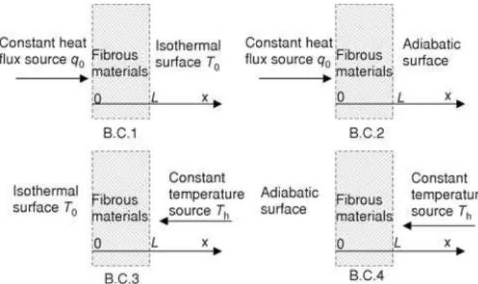
In the present work, several typical boundary conditions (B.C.) in porous material ap-plications are discussed, shown in fig. 2 corresponding to the mathematical forms in tab. 1. Both B.C.1 and B.C.2 are the representa-tive cases under the constant heat sources, while B.C.3 and B.C.4 are heated by the constant temperature sources in fig. 2. Their initial condi-tions are all set as the same temper-ature T₀. The processes of solving the above governing equations un-der the B.C.1-4, respectively, are provided in the Appendix by em-ploying an analytical method [7], where the dimensionless tempera-ture distributions for each phase have been obtained.

Table 1. four different boundary conditions

B.C.1 B.C.2 B.C.3 B.C.4

x= 0 k T

x k

T

x q

a a f f

¶

¶ ¶

¶

= = - ₀ k T

x k

T

x q

a a f f

¶

¶ ¶

¶

= = - ₀ T_a =T_f =T₀ ¶ ¶

¶

¶ T

x T

x

a ₌ f ₌₀

x=L T_a=T_f =T₀ ¶

¶ ¶

¶ T

x T

x

a ₌ f _{=0 T T T}

a= f = h Ta=Tf =Th

Initial condition

t= 0 Ta=Tf =T0 Ta=Tf =T0 Ta =Tf =T0 Ta=Tf =T0

A criterion of local thermal equilibrium in fibrous materials

Once obtaining the temperature distribution for each phase, we can facilely obtain the local discrepancy between the contacting phases in the localized representative volume. This discrepancy solely determines the internal LTE behavior,i. e., the bigger the discrepancy, the deeper the system into the LTNE condition. The local discrepancy D_{q between the} dimensionless temperature distributions of the two phases can be expressed as:

D_q=_q -_q

a f (4)

whereq_aandq_fare the dimensionless temperatures for the air and fiber phases derived from Ap-pendix. Therefore, the porous material can be treated as in the LTE conditions once this discrep-ancyD_q<D_q

cv,i. e., becoming smaller than a critical valueDqcv(= 0.0001 in our study).

In our discussions below, the isothermal case B.C.1 is chosen as an example to study the local discrepancyD_{qbetween the thermal states of the two phases. The sample thicknessL} and heat source fluxq₀are set at 0.01m and 100 W/m2_{, the fiber volumetric heat capacityrC}

fis

5·105 _J/m3_{K and the properties of the air phase are given as k}

a= 0.025 W/mK and rCa =

=1.21·103_J/m3_{K from ref. [28, 29]. Other parameters at the default values are in tab. 2.}

Table 2. The properties used in computation

Physical property Fiber phase kf[Wm–1K–1]

Pore hydraulic radiusrh[m]

Fiber phaser Cf[Jm–3K–1]

Porosity

e

Default value 0.10 5.0·10–4 _1.0·105 _0.80

Range 0.05~2.50 5.0·10–5_~1.0·10–3 _2.0·103_~1.0·106 _0.05~0.95

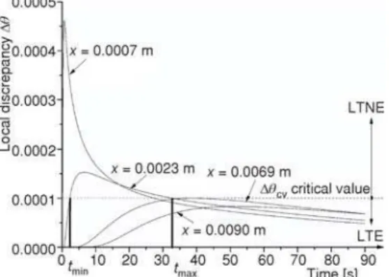
The local discrepancy curvesD_{qin fig. 3,} il-lustrate the phase-lag in temperature of the sam-ple against time, at different locations x. The curves exhibit a similar trend, increasing from the origin, reaching the peaks and then falling off to zero. We can then define two time mark-ers (t_minandt_max) between the curves using the critical valueD_q

cv, so as to symbolize the entry

and exit moments of the LTNE condition. The net length between these two moments (D_{t =} =it_max –t_min) represents the duration stayed in the LTNE condition. Thus the two time points (t_minandt_max) and the duration (D_{t) can be used} logically as the parameters to assess the LTE condition of a porous system. Here, intrinsi-cally,D_{t, the duration of LTNE, characterizes} the effective transit period of the entire heat

transfer process, and the rest time can be treated as in the LTE state, including the steady-state period and the residual transient period, with negligible marginal local discrepancyD_q<D_q

cv.

These two time markers are clearly functions of many related variables:

t f k C r T

t T t f k C

min = , , , , , , max , , æ

è

ç ö

ø

÷ =

1 f r f e h a st* 2 f r f

¶

¶ e,r , ,

T t T h a st*

¶

¶

æ è

ç ö

ø

÷ (5)

whereT_st* _{is the steady-state temperature in each boundary case made available in Appendix.}

That is, these two parameters are not only related to the intrinsic properties of the material sys-tem (fiber phase thermal conductivityk_f, volumetric heat capacityrC_f, porositye, and pore hy-draulic radiusr_h) but also to the temperature slope ¶_T

a/¶t andTst*.

Returning to fig. 3 where four curves of the same sample are shown, corresponding to different locations in the samplex = 0.0007 m, 0.0023 m, 0.0069 m, and 0.0090 m, it is clear first that in the same sample but at the locations sufficiently further away from the heat source (x³0.0069 m), the system is always at the LTE condition throughout the time based on the crite-rionDq<D_q

cvso that the local temperature discrepancy between the air and solid fiber can be

neglected. It is only at the locations withinx< 0.0069 m that LTNE becomes a concern – the

closer the location,i. e., a smallerx, the earlier for the location to enter LTNE state. In other words, during a thermal transfer process in a porous material with constant heat source, only the parts close enough to the heat source experience the local thermal non-equilibrium state.

Thermal responses at different boundary conditions

In this section, the equilibrium status of both boundary (isothermal/adiabatic), and heat source conditions (constant heat flux/temperature) listed in fig. 2 are discussed so as to ex-hibit the differences between them. We then found out from our calculations that not only such differences are huge, but they depend on the fiber thermophysical properties (k_fandrC_f) and sample structure properties (e) as well. Nonetheless a complete graphic illustration of such in-fluence of different boundary conditions, at all possible ranges of the properties, is too complex to present in one drawing, we only provided a few special cases with some fixed properties in figs. 4 and 5, just to show the differences. Whereas simpler cases hence with more comprehen-sive illustrations are shown in figs. 7 in 3-D plotting where one can get the sense of the difficul-ties involved.

The distributions oft_min,t_max, andD_{tfor B.C.1~4 are illustrated in figs. 4 and 5 using the} boundary conditions listed in tab. 1 and the data in tab. 2. Conditions B.C.1 and 2 are both heated by the same constant heat flux source (q₀= 100 W/m2_{), while B.C.3 and 4 by the constant}

tempera-ture source (T_h= 10 °C). The initial temperature of these four cases are all set asT₀= 0 °C. First, in both B.C.1 and 2 cases in fig. 4(a) and (b),t_min,t_maxandD_{tsimultaneously} in-crease against the distancex, meaning that at locations further away from the heat source (x= 0), the entry (t_min) and exit (t_max) moments to LTNE stage are both delayed, and the duration (D_{t) in} LTNE is extended.

From fig. 4(a) and (b), we can also conclude that the isothermal case B.C.1 possesses a greater tmin but smaller tmax than the adiabatic case B.C.2, resulting in a much shorter duration D_{t. The differences are attributed to the nature of the boundary settings: at the isothermal} condi-tion B.C.1 with a higher heat leaking from the other end, the sample is only able to retain a lower temperature level, unlike the adiabatic B.C.2 surface where no heat leaks out at all.

Whereas for B.C.3 and 4 boundary conditions with constant heat temperature source (T_h= 10 °C), assuming the source located atx= 0.01 m, at that point both the fiber and air phases

possess the same temperature (T_f =T_a=T_h) and thus always at LTE condition. Once moving away from the heat source however, seen from fig. 5(a), the samples enter the LTNE state. Over-all, the isothermal case B.C.3 stays in the LTNE state shorter, indicated by a smallerD_{tvalue in} fig. 5(a), but enters and leaves the LTNE state earlier, by smallert_minandt_maxvalues in fig. 5(b), than the adiabatic B.C.4 case. The results can be explained in thermal physics terms. Since the isothermal B.C.3 surface leaks more heat than the B.C.4 case, it thus requires greater heat supply from the heat source to maintain its constant temperature (T_h) at the other end. Such heat has to be transferred through the same material over the same distance from the heat source, the heat transfer rate in B.C. 3 has to be higher so that both the entry time (t_min) and exit time (t_max) of LTNE in B.C.3 are earlier than those in B.C.4, leading to overall a smaller durationD_{tthan in} B.C.4.

Furthermore, as the thermal responses of samples under convection boundaries are considered to be all within the isothermal and adiabatic boundary conditions [30], the LTE state for such convection cases can also be estimated here based on the two extreme cases. That is, the isothermal and adiabatic boundaries can be viewed as the special cases of all the convection boundary cases, with the maximum and minimum convection coefficients, respectively. For all convection situationst_min,t_maxandD_{t are located between these two bounds as indicated in figs.} 4(b) and 5(b), where region A are the corresponding LTNE entry moments (t_min), and Region B are the estimated exit moments (t_max) for all the convection cases.

The boundary conditions of actual fibrous materials are more complex than the cases dealt with here,e. g., with different initial conditions of internal phases, samples with three or more phases, and multi-dimension heat transfer,etc., and their corresponding LTE status will be more erratic. But the approach proposed in this paper can still be useful as an approximate and simply way to study the LTE behaviors of these complex cases.

Effects of several key parameters on the sample LTE behavior

In this section, the influences of the fiber thermophysical properties (k_fandrC_f) and sample porosityeand pore hydraulic radiusr_hon the system parameters (t_min, t_max, andD_{t) are} discussed, again using B.C.1 as the example. The ranges of the related parameters in our

tation are from tab. 2: when dealing with one parameter, others will always take the default val-ues, and the heat source fluxq₀is fixed at 100 W/m2_.

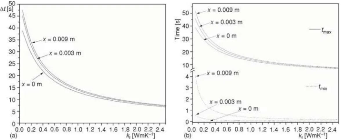
Influence of the fiber thermal conductivity

The fiber thermal conductivityk_fwithin the range in tab. 2 is used to calculate the re-sults drawn in fig. 6. The value ofD_{tdecreases with the increasedk}

fin fig. 6(a), and the other two

parameters (t_minandt_max) in fig. 6(b) exhibit the similar trend. The influence of sample locationx as seen from the curves is also quite simple.

Thermal conductivity by definition is the specific amount of the heat that passes the cross-section of an object. Since in B.C.1 case with constant heat supply for the porous sample, the sample with biggerk_fcan thus transfer heat more quickly to the entire sample, so its tempera-ture rises earlier and the slope becomes steeper, leading to a smaller entry time (t_min). However, as this high transfer ability will also leak more heat to the external environment more quickly and thus more difficult to maintain the temperature, it leads to an end moment (t_max) earlier than the sample with smallerk_f. In other words, the fiber thermal conductivity is an important factor in affecting the LTE conditions, the higher thek_fvalue, the earlier LTNE appears, but overall the shorter LTNE period for the sample. Also, remembering what demonstrated in the sectionA cri-terion of local thermal equilibrium in fibrous materials, the curves oft_minandt_maxhere can be used as the limitting cases for the convection problems.

Influence of fiber volumetric heat capacity

The influence of fiber volumetric heat capacityrC_fis given in fig. 7, in 3-D due to the complicities caused by having to include the sample locationxas well. It is shown in fig. 7(a) that, locationxexerts a significant impact on the LTNE durationD_{t: when the location in the} sample is sufficiently further away from the heat source (x

_o

0), the sample will not experience the LTNE state at all as long as the sample volumetric heat capacityrC_fis not too small. How-ever, at other locationx, the influence ofrC_fonD_{tshows a parabola pattern:}D_{tincreases from} zero to a maximum and then drops back to near zero asrC_fdecreases from its maximum to close to 0.

Correspondingly, the influences of both positionxandrC_fon the entry timet_minin fig. 7(b) are very similar to fig. 7(a) onD_{t. Whereas the profiles on the exit timet}

maxis such that

com-bined with those fort_min, an unsymmetrical tubular 3-D hyper-plane is formed where two parab-ola curved planes fort_minandt_maxconnected at a critical line, meaning the entry and exit mo-ments converge (t_min = t_max) and the LTNE duration degenerates to zero. Note the 3-D connecting critical line is projected into the 2-D line in fig. 7(b).

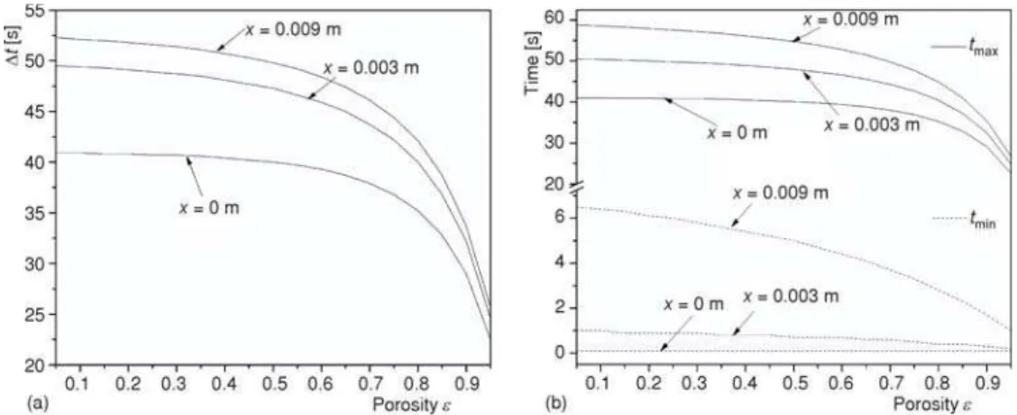
The influence of sample porosity

Porositye, a key parameter of material structure, is specified in this section and its re-lationship with the characteristic parameters is plotted in fig. 8. Porosityeis defined as the frac-tion of the volume of voids over the total volume. In a porous material, increasingeor the air volume fraction shifts the thermal response of the material towards more dominance by the air phase which possesses significantly smaller thermal conductivity and volumetric heat capacity than the fiber phase. Hence, heated by the constant heat flux in B.C.1, the samples with greater porosity holding more air will experience a quicker temperature rise and reach the steady-state condition earlier,i. e., the corresponding timest_minandt_maxboth arrive earlier and the duration D_{ttends to be smaller, as illustrated in figs. 8(a) and (b).}

Figure 7. Effect of the fiber volumetric heat capacityrCfon the parameters, (a) forDtand (b) fortminand

tmax

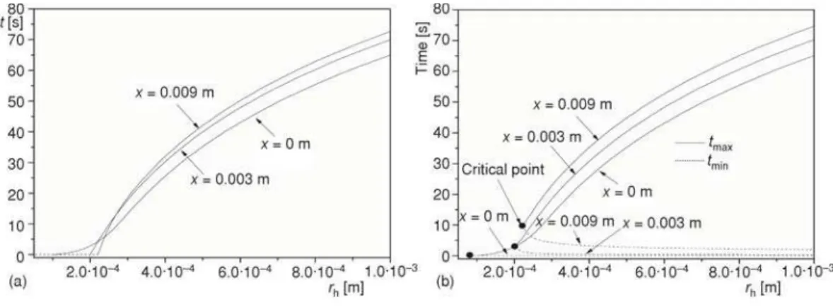
The influence of sample pore hydraulic radius

Pore hydraulic radiusr_hplays an important role inD_{t, and also impacts ont}

minandtmax

from fig. 9(a) and (b). D_{t and t}

max are both proportionate to the rh while tmin with the

in-versely-proportional relationship. A biggerr_h=D_V

p/DApmeans that the specific contacting

sur-faces between local air and fiber phase are smaller, so the heat exchange may be more ineffi-cient, according to eq. (2), then the time of local discrepancy increasing to the critical valueD_q

cv

becomes earlier and decreasing toD_q

cvbecomes later, so tmin andtmax, respectively, become

smaller and bigger with a largerr_h. We also can find thatt_minandt_maxoverlap at the critical line, which means that the LTNE can be avoided once ther_his small enough.

Conclusions

By using the heat transfer theory for fibrous porous materials, we calculated the local discrepancy of adjacent two phases (air/fiber) to establish a criterion; this criterion can be used to determine the LTE condition for porous media, using three characteristic parameters, the en-try and exit moments of LTNEt_minandt_max, and the duration in LTNE stageD_t.

Four common boundary conditions were employed to study the influence of boundary conditions. Heated by the same constant heat flux source, the isothermal case possessed a bigger t_minand smallert_maxthan the adiabatic case, so the former enters LTNE later and stays there for a short periodD_{tthan the latter. Under the constant temperature source, the isothermal model is in} and out of the LTNE stage earlier than the adiabatic one, resulting an overall shorter durationD_t.

The isothermal and adiabatic boundaries can be viewed as the special cases of all the convection boundary cases, with the maximum and minimum convection coefficients, respec-tively. For all convection situationst_min,t_max, andD_{tare located between these two bounds. In} other words, the LTNE behavior of convection boundaries could be generally estimated from the region rounded by the two bounds (isothermal/adiabatic).

As to the influences of the fiber thermophysical properties (k_fandrC_f) and material porosityeand pore hydraulic radiusr_hon thermal behaviors of porous media, increasing any one ofk_f,rC_f, andewill reduce and even eliminate the region of LTNE status in the case (iso-thermal with constant heat flux) conditions. Our theoretical approach can be extended to assess the LTE conditions of some other complex, dynamic, and multiscale cases.

Acknowledgment

Financial support of this work was provided by Natural Science Foundation of China via grant no. 51306095 and 51273097 and Taishan scholars construction engineering of Shandong province.

Appendix

This appendix details the solution of the governing equations eqs. (1)-(3) under four different boundary conditions listed in tab. 1 and fig. 2. The temperature distribution of each model can be derived as follow based on the analytical approach [7]. In the present work, the boundary conditions are considered as the non-flow or negligible flow cases, therefore the natu-ral convection can be ignored genenatu-rally [31, 32] if there is no flow blow-in from the boundaries.

The air phase solution ofB.C.1can be solved as:

T

q n x

L CL

a a

q e n

n n n e = + é ëê ù ûú + - + +

0 2 1

2 2

cos ( )

( )

( ) (

p

r t t w

w w w _w w

w

n n n n

n n e

- - + = -é ë ê ù û ú

å

a t a t

n n n a a ) _{( )} ( ) 2 2 0 4 (A.1a)

The fiber phase temperature distribution can be solved from the relation defined in eq. (2), in addition, the interstitial heat transferh_ecan be replaced ash_e= Nu_rhk_a/r_h, the Nusselt num-ber Nu_rhis about 1 andt_qis set as zero, in the no flow case of ref. [7], so:

T T r C h

T t T

r C k

q n x

L

a h

f a h a e a a rh a Nu = + = + + é

r ¶ r

¶

p

2 0 2 1

2

cos ( )

ëê ù ûú + - - + =

å

(e n n e n n

q e n

( ) ( )

( )

w w

r t t w

a t a t

n 0 CL

4

(A.1b)

We then obtain the dimensionless temperature distribution of each phase:

q_a st a q

st

f st f st =T -T =

-T

T T

T (A.1c)

where symbols Nomenclature

DAp – pore surface area, [m 2

]

aaf – specific surface area of porous materials, – [m–1]

Fn(x) – eigenfunction

he – interstitial heat transfer coefficient, – [Wm–2K–1]

k – thermal conductivity, [Wm–1K–1] L – porous material thickness, [m]

Nn – norm

q(x, t) – heat flux, [Wm–2]

rh – hydraulic radius,DVp/DAp, [m]

S – volumetric heat source, [Wm–3] tmin – entry moment to the LTNE condition, [s]

tmax – exit moment to the LTNE condition, [s]

Dt – duration of the LTNE condition, [s] T(x, t) – temperature distribution, [K] T0 – initial temperature, [K]

T_st* – steady-state temperature, [K] r

U – velocity vector of fluid, [ms–1] DVp – volume of a mean pore, [m

3

] x – space co-ordinate in x-direction, [m]

Greek symbols

e – porosity of porous materiale=Va/V q – dimensionless temperature

gn – eigenvalue

rC – heat capacity/unit volume, [Jm–3K–1]

tt – lag time of the temperature gradient [s] tq – lag time of the heat flux [s]

te – [= (1 –e)(rC)ftt/rC]

Subscripts

a_{n n n n n n n n} t

q e n q e

= - - =

-+ - +

é

ë ê

g b w b l b g t

t t g t t

, ,

( )

2 2 ₁ 1

2

1 2

ù

û

ú,l =g - t₊

t t

n n t

q e

1

and

T

q n x

L

CL _n a_n

n

st

q e n

n = + é ëê ù ûú + -= 0 2 2 2 1 2 2

cos ( )

( )

p

r t t w

w w

0

4

å

is the final steady-state temperature after non-linearly rise of the transient stage. The parameters (F_n(x),N_n, andg_n) can be acquired and yielded in tab. A.1 under different boundary conditions.

Table A.1. Calculated parameters for each boundary condition

Eigenfunction Fn(x) (n= 0, 1, 2, ...)

Eigenvalue

gn(n= 0, 1, 2, ...)

NormNn

B.C.1 Fn(x) = cos((2n+ 1)px/2L) gn= [(2n+ 1)p/2L] 2

ke/rC Nn=L/2

B.C.2 Fn(x) = cos(npx/L) gn= (np/L)2ke/rC Nn=L n= 0Nn=L/2n> 0

B.C.3 Fn(x) = sin(npx/L) gn= (np/L) 2

ke/rC Nn=L/2

B.C.4 Fn(x) = cos((2n+ 1)px/2L) gn= [(2n+ 1)p/L)2ke/rC Nn=L/2

Furthermore, the derivation of others three models (B.C.2~4) can be found as follow.

B.C.2.

The temperature distribution of air phase and fiber phase can be obtained:

T q CL a t a q n a a t = - + + + + + ì í ïï î ï ï + - +

0 0 0

0 0

0

1 0 0

r w w w ( ) cos ( ) e p_x

L a a

n ant n ant

æ è ç ö ø ÷ -_[ +₍ + ₎ - +₍ - ₎ - + ( ( ) ( )

2w w w w w

n n n e n n e

t_q +t w_{e n} w

-ü ý ïï þ ï ï =

å

_{) ( )}

n n

n 1 2 a2

4

(A.2a)

T T r C

k q

CL

q n x L

h a t

f a a rh a Nu e = + - + æ è ç ö - + 2 0 0

1 0 0

r r w ( cos ( ) p ø ÷ -+ é ë ê ù û ú ì í ïï î - - + =

å

_r w _{t t w}w

CL

n an t n ant

n

e e

q e n ( ) ( ) ( ) 1 4 ï ï ü ý ïï þ ï ï (A.2b)

The dimensionless temperature distribution:

q_a ast a q

ast

f fst f fst

=T -T =

-T T T T , (A.2c) where T_ast n q = - + + + + - æ è ç ö ø ÷ + q CL a t a n x L

0 0 0

0 0 1 2 r w w w t

( ) ( ) cos

(

p

t w_e) _n(w_{n n})

n 1 2 -a2

T_fst

rh a

n

Nu

= á ñ +- + +

+ + -q CL r C k a t a h a

0 2 0 0

0 0 1 2 r r w w w

( ) ( ) cos

( ) ( )

n x L

a

n n n

n p æ è ç ö ø ÷ + -é ë ê ê ê ê ù û ú ú ú ú =

å

_{t t w w}

q e 2 2

1

4

are the

linear temperatures arising during the quasi-steady stage of air and fiber phase, respectively.

B.C.3

T T L x

T n x L n

a n

h _{a t}

n n

a h n n

e = + - æ è ç ö ø ÷ + -

-2( 1) sin

( ) ( ) (

p

p

w w w

n n a t

n

a n n

2 2 1 2 -ì í î ü ý þ + =

å

)_e( )

n

w

w

4

(A.3a)

T T r C k

T n x L n a h n h n n f a a rh a Nu = + - æ è ç ö ø ÷ -2_r 2( 1) sin _(w2 2₎

p

p

e e

n

(w ) _{(w )} (w )

w

n ant n n

n n a t

n a - - + = - -é ë ê ù û ú ì í ïï î ï ï

å

2 2

1 2 4 ü ý ïï þ ï ï(A.3b)

The final temperature value of this model isT_f(x) =T_a(x) =T_hx/L, so the dimensionless temperature distribution:

q_a h a q

h

f h f h =T x-T L =

-T x

T x T L T x

, (A.3c)

B.C.4

T T

T n x

L n+

a n

h

a h n n

e

=

-- é +

ëê

ù

ûú +

2 1 2 1

2

2 1

( ) cos ( )

( )

( ) (

p

p

w wn ant n ant

n a - - + = + -ì í î ü ý þ

å

) _{(w )} ( )

w w n n n e 1 4 (A.4a)

T T r C k

T n x

L n h n h f a a rh a Nu =

-- é +

ëê

ù ûú +

2 2 1 2 1 ₂

2 1

r ( ) cos ( )

( p ) ( ) ( ) ( ) ( ) p w w w w w

n n a t n n a t

n

a n n a n n

2 - 2 - 2 - 2 é ë ê ù û ú - - + = e e n 1 4

å

ì í ïï î ï ï ü ý ïï þ ï ï (A.4b) The dimensionless temperature distribution:

q_a h a q

h

f h f h

=T -T =

-T

T T T

, (A.4c)

References

[1] Cattaneo, C., About Heat Conduction (in Italian), Atti del Semin, Mat.e Fis. Univ. Modena,3(1948), pp. 83-101

[2] Vernotte, P., Paradoxes in the Continuous Theory of the Heat Equation,C. R. Acad. Bulg. Sci., 246(1958), pp. 3154-3155

[3] Tzou, D. Y., A Unified Field Approach for Heat Conduction From Macro- to Micro-Scales,Journal of Heat Transfer, 117(1995), 1, pp. 8-16

[4] Amiri, A., Vafai, K., Analysis of Dispersion Effects and Non-Thermal Equilibrium, Non-Darcian, Vari-able Porosity Incompressible Flow through Porous Media,International Journal of Heat and Mass Trans-fer, 37(1994), 6, pp. 939-954

[5] Nield, D.A.,et al., Effect of Local Thermal Non-Equilibrium on Thermally Developing Forced Convec-tion in a Porous Medium,International Journal of Heat and Mass Transfer, 45(2002), 25, pp. 4949-4955 [6] Kuznetsov, A. V., An Investigation of a Wave of Temperature Difference between Solid and Fluid Phases

[7] Minkowycz, W. J.,et al., On Departure from Local Thermal Equilibrium in Porous Media Due to a Rap-idly Changing Heat Source: the Sparrow Number,International Journal of Heat and Mass Transfer, 42 (1999), 18, pp. 3373-3385

[8] Lee, D.Y., Vafai, K., Analytical Characterization and Conceptual Assessment of Solid and Fluid Temper-ature Differentials in Porous Media,International Journal of Heat and Mass Transfer, 42(1999), 3, pp. 423-435

[9] Yang, K.,et al., Analysis of Temperature Gradient Bifurcation in Porous Media – An Exact Solution, In-ternational Journal of Heat and Mass Transfer, 53(2010), 19-20, pp. 4316-4325

[10] Vadasz, P., On the Paradox of Heat Conduction in Porous Media Subject to Lack of Local Thermal Equi-librium,International Journal of Heat and Mass Transfer, 50(2007), 21-22, pp. 4131-4140

[11] Zhao, L.,et al., Fractal Approach to Flow through Porous Material,International Journal of Nonlinear Sciences and Numerical Simulation, 10(2009), 7, pp. 857-902

[12] Shi, X.-J., Yu, W. D., Fractal Phenomenon in Micro-Flow through a Fiber Bundle,International Journal of Nonlinear Sciences and Numerical Simulation, 10(2009), 7, pp. 861-866

[13] Li, Z.-B., He, J.-H., Fractional Complex Transform For Fractional Differential Equations,Mathematical and Computational Application, 15(2010), 5, pp. 970-973

[14] Li, Z.-B., An Extended Fractional Complex Transform,International Journal of Nonlinear Sciences and Numerical Simulation, 11(2010), Suppl., pp. 135-337

[15] He, J.-H., A New Fractal Derivation,Thermal Science, 15(2011), Suppl. 1, pp. S145-S147

[16] Fan, J.,et al., Hierarchy of Wool Fibers and Fractal Dimensions,International Journal of Nonlinear Sci-ences and Numerical Simulation, 9(2008), 3, pp. 293-296

[17] Yang, X.-J., et al., Fractal Heat Conduction Problem Solved by Local Fractional Variation Iteration Method,Thermal Science, 17(2012), 3, pp. 707-713

[18] Lee, J.,et al., Effect of Thermal Non-Equilibrium on Convective Instability in a Ferromagnetic Fluid-Sat-urated Porous Medium,Transport In Porous Media, 86(2011), 1, pp. 103-124

[19] Nouri-Borujerdi, A.,et al., The Effect of Local Thermal Non-Equilibrium on Conduction in Porous Chan-nels with a Uniform Heat Source,Transport in Porous Media, 69(2007), 2, pp. 281-288

[20] Hayes, A. M.,et al., The Thermal Modeling of a Matrix Heat Exchanger Using a Porous Medium and the Thermal Non-Equilibrium Model, International Journal of Thermal Sciences, 47 (2008), 10, pp. 1306-1315

[21] Tian, M.,et al., Measuring the Thermophysical Properties of Porous Fibrous Materials with a New Un-steady-State Method,Journal of Thermal Analysis and Calorimetry, 107(2012), 1, pp. 395-405 [22] Xu, F., et al., Modeling Skin Thermal Pain Sensation: Role of Non-Fourier Thermal Behavior in

transduction Process of Nociceptor,Computers in Biology and Medicine, 40(2010), 5, pp. 478-486 [23] Tian, M., et al., Skin Thermal Stimulation on Touching Cool Fabric from the Transient Stage to

Steady-State Stage,International Journal of Thermal Sciences, 53(2012), March, pp. 80-88 [24] Pan, N.,et al., Fibrous Materials as Soft Matter,Textile Res. J., 77(2007), 4, pp. 205-213

[25] Wang, X. Y.,et al., Abrasion Resistance of Thermally Bonded 3D Nonwoven Fabrics,Wear, 262(2007), 3-4, pp. 424-431

[26] Amiri, A.,et al., Transient Analysis of Incompressible Flow through a Packed Bed,International Journal of Heat and Mass Transfer, 41(1998), 24, pp. 4259-4279

[27] Wang, L.,et al., Equivalence between Dual-Phase-Lagging and Two-Phase-System Heat Conduction Pro-cesses,International Journal of Heat and Mass Transfer, 51(2008), 7-8, pp. 1751-1756

[28] Kim, K. J.,et al., Thermal Conduction between a Heated Microcantilever and a Surrounding Air Environ-ment,Applied Thermal Engineering, 29(2009), 8-9, pp. 1631-1641

[29] Tian, M.,et al., Effects of Layer Stacking Sequence on Temperature Response of Multi-Layer Composite Materials under Dynamic Conditions,Applied Thermal Engineering, 33-34(2012), Feb., pp. 219-226 [30] Hammerschmidt, U., A Quasi-Steady State Technique to Measure the Thermal Conductivity,

Interna-tional Journal of Thermophysics, 24(2003), 5, pp. 1291-1312

[31] Farnworth, B., Mechanisms of Heat Flow through Clothing Insulation Textile Research Journal, 53 (1983), 12, pp. 717-725

[32] Tian, M.,et al., Effects of Layering Sequence on Thermal Response of Multilayer Fibrous Materials: Un-steady-State Cases,Experimental Thermal and Fluid Science, 41(2012), Apr., pp. 143-148