Submitted 13 February 2015 Accepted 6 May 2015 Published27 May 2015 Corresponding author Mikael Vejdemo-Johansson, [email protected]
Academic editor Anne Bergeron
Additional Information and Declarations can be found on page 13
DOI10.7717/peerj-cs.2
Copyright 2015 Hirsch et al.
Distributed under
Creative Commons CC-BY 4.0
OPEN ACCESS
More ties than we thought
Dan Hirsch1, Ingemar Markstr¨om2, Meredith L. Patterson1, Anders Sandberg3and Mikael Vejdemo-Johansson2,4,5 1Upstanding Hackers Inc.
2KTH Royal Institute of Technology, Stockholm, Sweden 3Oxford University, UK
4Joˇzef ˇStefan Institute, Ljubljana, Slovenia
5Institute for Mathematics and its Applications, Minneapolis, USA
ABSTRACT
We extend the existing enumeration of neck tie-knots to include tie-knots with a textured front, tied with the narrow end of a tie. These tie-knots have gained popularity in recent years, based on reconstructions of a costume detail from The Matrix Reloaded, and are explicitly ruled out in the enumeration byFink & Mao (2000). We show that the relaxed tie-knot description language that comprehensively describes these extended tie-knot classes is context free. It has a regular sub-language that covers all the knots that originally inspired the work. From the full language, we enumerate 266,682 distinct tie-knots that seem tie-able with a normal neck-tie. Out of these 266,682, we also enumerate 24,882 tie-knots that belong to the regular sub-language.
Subjects Algorithms and Analysis of Algorithms, Computational Linguistics, Theory and Formal Methods
Keywords Necktie knots, Formal language, Automata, Chomsky hierarchy, Generating functions
INTRODUCTION
There are several different ways to tie a necktie (Fig. 1). Classically, knots such as the four-in-hand, the half windsor and the full windsor have commonly been taught to new tie-wearers. In a sequence of papers and a book,Fink & Mao (2001),Fink & Mao (2000) andFink & Mao (1999)defined a formal language for describing tie-knots, encoding the topology and geometry of the knot tying process into the formal language, and then used this language to enumerate all tie-knots that could reasonably be tied with a normal-sized necktie.
The enumeration of Fink and Mao crucially depends on dictating a particular finishing sequence for tie-knots: a finishing sequence that forces the front of the knot—the fac¸ade—to be a flat stretch of fabric. With this assumption in place, Fink and Mao produce a list of 85 distinct tie-knots, and determine several novel knots that extend the previously commonly known list of tie-knots.
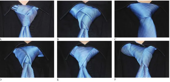
Figure 1 Some specific tie-knot examples. Top row from left: the Trinity (L-110.4), the Eldredge (L-373.2) and the Balthus (C-63.0, the largest knot listed by Fink and Mao). Bottom row randomly drawn knots. From left: L-81.0, L-625.0, R-353.0.
a knot with textures or stylings of the front of the knot, producing symmetric and pleasing patterns.
Knorr (2010)gives the history of the development of novel tie-knots. It starts out in 2003 when theedeity knotis published as a PDF tutorial. Over the subsequent 7 years, more and more enthusiasts involve themselves, publish new approximations of the Merovingian tie-knot as PDF files or YouTube videos. By 2009, the new tie-knots are featured on the website Lifehacker and go viral.
In this paper, we present a radical simplification of the formal language proposed by Fink and Mao, together with an analysis of the asymptotic complexity class of the tie-knots language. We produce a novel enumeration of necktie-knots tied with the thin blade, and compare it to the results of Fink and Mao.
Formal languages
The work in this paper relies heavily on the language of formal languages, as used in theoretical computer science and in mathematical linguistics. For a comprehensive reference, we recommend the textbook bySipser (2006).
Recall that given a finite setLcalled analphabet, the set of all sequences of any length
of items drawn (with replacement) fromLis denoted byL∗. A formal languageon
the alphabetLis some subsetAofL∗. The complexity of the automaton required to
determine whether a sequence is an element ofAplacesAin one of several complexity
L
R
C
T
W
Thin
blade
Broad
blade
B A
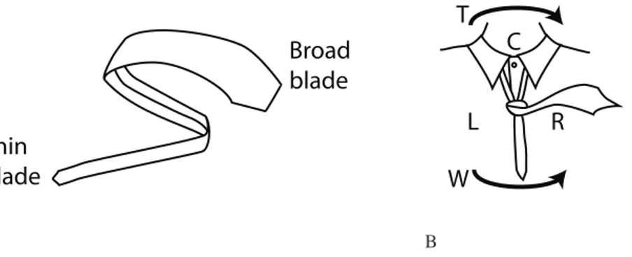
Figure 2 Left/Center/Right.The parts of a necktie, and the division of the wearer’s torso with the regions (Left, Center Right) and the winding directions (Turnwise, Widdershins) marked out for reference.
One way to describe a language is to give agrammar—a set of production rules that decompose some form of abstract tokens into sequences of abstract or concrete tokens, ending with a sequence of elements in some alphabet. The standard notation for such grammars is the Backus–Naur form, which uses::=to denote the production rules and
⟨some name⟩to denote the abstract tokens. Further common symbols are∗, the Kleene star, that denotes an arbitrary number of repetitions of the previous token (or group in brackets), and|, denoting a choice of one of the adjoining options.
THE ANATOMY OF A NECKTIE
In the following, we will often refer to various parts and constructions with a necktie. We call the ends of a necktieblades, and distinguish between thebroad bladeand thethin blade1—seeFig. 2for these names. The tie-knot can be divided up into abody, consisting of 1There are neckties without a width
difference between the ends. We ignore this distinction for this paper.
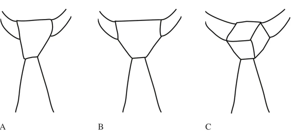
all the twists and turns that are not directly visible in the final knot, and afac¸ade, consisting of the parts of the tie actually visible in the end. InFig. 3we demonstrate this distinction. The body builds up the overall shape of the tie-knot, while the fac¸ade gives texture to the front of the knot. The enumeration of Fink and Mao only considers knots with trivial fac¸ades, while these later inventions all consider more interesting fac¸ades. As a knot is in place around a wearer, the Y-shape of the tie divides the torso into 3 regions: Left, Center and Right—as shown to the right inFig. 2.
A tie-knot has to be tied by winding and tucking one of the two blades around the other: if both blades are active, then the tie can no longer be adjusted in place for a comfortable fit. We shall refer to the blade used in tying the knot as theleading bladeor theactive blade. Each time the active blade is moved across the tie-knot—in front or in back—we call the part of the tie laid on top of the knot abow.
A LANGUAGE FOR TIE-KNOTS
Figure 3 Different examples of tie knots.Left, a 4-in-hand; middle, a double windsor; right a trinity. The 4-in-hand and double windsor share the flat fac¸ade but have different bodies producing different shapes. The trinity has a completely different fac¸ade, produced by a different wind and tuck pattern.
move to tuck the bladeUnder the tie itself.2The notation proposed byFink & Mao (2000)
2Fink and Mao usedTforTuck.
interprets repetitionsUkofUas tucking the bladekbows under the top. It turns out that the complexity analysis is far simpler if we instead writeUkfor tucking the blade under the bow that was produced 2kwindings ago. This produces a language on the alphabet:
{L⊗,L⊙,C⊗,C⊙,R⊗,R⊙,U}
They then introduce relations and restrictions on these symbols:
Tie1 No region(L,C,R)shall repeat: after anLonlyCorRare valid next regions.U moves do not influence this.
Tie2 No direction (⊙—out of the paper,⊗—in towards the paper) shall repeat: after an outwards move, the next one must go inwards.U moves do not influence this.
Tie3 Tucks (U) are valid after an outward move.
Tie4 A tie-knot can end only on one ofC⊗,C⊙orU. In fact, almost all classical knots end onU.3
3The exemption here being the Onassis
style knot, favored by the eponymous shipping magnate, where after a classical knot the broad blade is brought up with aC⊙move to fall in front of the knot, hiding the knot completely.
Tie5 Ak-fold tuckUkis only valid after at least 2kpreceding moves.Fink & Mao (2000)do not pay much attention to the conditions onk-fold tucks, since these show up in their enumeration as stylistic variations, exclusively at the end of a knot.
This collection of rules allow us to drastically shrink the tie language, both in alphabet and axioms. Fink & Mao are careful to annotate whether tie-knot moves go outwards or inwards at any given point. We note that the inwards/outwards distinction follows as a direct consequence of axiomsTie2,Tie3andTie4. Since non-tuck moves must alternate between inwards and outwards, and the last non-tuck move must be outwards, the orientation of any sequence of moves follows by backtracking from the end of the string.
Hence, when faced with a non-annotated string like
we can immediately trace from the tail of the knot string: the last move before the final tuck must be outwards, so thatLmust be aL⊙. So it must be preceded byR⊙C⊗. Tracing backwards, we can specify the entire string above to
R⊗C⊙L⊗C⊙R⊗C⊙L⊗C⊙R⊗C⊙L⊗R⊙UC⊗R⊙C⊗L⊙U
Next, the axiomTie1means that a sequence will not contain either ofLU∗L,CU∗C,RU∗R as subsequences.4Hence, the listing of regions is less important than the direction of 4Recall that the Kleene starF∗is used
to denote sequences of 0 or more repetitions of the stringF.
transition: any valid transition is going to go either clockwise or counterclockwise.5
5Say, as seen on the mirror image.
Changing this convention does not change the count, as long as the change is consequently done.
WritingTfor clockwise6andWfor counterclockwise,7we can give a strongly reduced
6Tfor Turnwise.
7Wfor Widdershins.
tie language on the alphabetT, W, U. To completely determine a tie-knot, the sequence needs a starting state: an annotation on whether the first crossing of a tie-knot goes across to the right or to the left. In such a sequence, aUinstruction must be followed by eitherTor Wdictating which direction the winding continues after the tuck, unless it is the last move of the tie: in this case, the blade is assumed to continue straight ahead—down in front for most broad-blade tie-knots, tucked in under the collar for most thin-blade knots.
The position of the leading blade after a sequence ofW/Twindings is a direct result of #W−#T(mod 3). This observation allows us to gain control over several conditions determining whether a distribution ofUsymbols over a sequence ofW/Tproduces a physically viable tie-knot.
Theorem 1.A position in a winding sequence is valid for a k-fold tuck if the sub-sequence of the last2kWorTsymbols is such that either
1. starts withWand satisfies#W−#T=2(mod 3)
2. starts withTand satisfies#T−#W=2(mod 3).
Proof.The initial symbol produces the bow under which the tuck will go. If the initial symbol goes, say, fromRtoL, then the tuck move needs to come fromCin order to go under the bow. In general, a tuck needs to come from the one region not involved in the covering bow. Every other bow goes in front of the knot, and the others go behind the knot. Hence, there are 2k−1 additional winding symbols until the active blade returns to the right side of the knot. During these 2k−1 symbols, we need to transition one more step around the sequence of regions. The transitionsWandTare generator and inverse for the cyclic group of order 3, concluding the proof.
It is worth noticing here that a particular point along a winding can be simultaneously valid for both ak-fold and anm-fold tuck fork̸=m. One example would be in the winding stringTWTT: ending withTT, it is a valid site for a 1-fold tuck producingTWTTU, and since TWTTstarts withTand has 2 moreTthanW, it is also a valid site for a 2-fold tuck producing TWTTUU. We will revisit this example below, in ‘Recursive tucks.’
be relevant; 4 for the broad blade ties. The bound of 4 is achieved in the enumeration by Fink & Mao (1999).
In our enumeration, we will for the sake of comfort focus on ties up to 13 moves.
LANGUAGE COMPLEXITY
In this section, we examine the complexity features of the tie-knot language. Due to the constraints we have already observed on the cardinality ofWandT, we will define a grammar for this language. We will write this grammar with a Backus–Naur form. Although in practice it is only possible to realise finite strings in the tie-knot language due to the physical properties of fabric, we assume an arbitrarily long (but finite), infinitely thin tie.
Single-depth tucks
The classical Fink and Mao system has a regular grammar, given by
⟨tie⟩ ::=L⟨L⟩
⟨lastR⟩ ::=L⟨lastL⟩ |C⟨lastC⟩ |LCU
⟨lastL⟩ ::=R⟨lastR⟩ |C⟨lastC⟩ |RCU ⟨lastC⟩ ::=L⟨lastL⟩ |R⟨lastR⟩
We use the symbol⟨lastR⟩to denote the rule that describes what can happen when the last move seen was anR. Hence, at any step in the grammar, some tie knot symbol is emitted, and the grammar continues from the state that symbol was the last symbol emitted.
The above grammar works well if the only tucks to appear are at the end. For intermediate tucks, and to avoid tucks to be placed at the back of the knot (obeyingTie3), we would need to keep track of winding parity: tucks are only valid an even number of winding steps from the end.
We can describe this with a regular grammar. For the full tie-knot language, the grammar will end up context-free, as we will see in ‘Recursive tucks.’
⟨tie⟩ ::= ⟨prefix⟩(⟨pair⟩ | ⟨tuck⟩)∗ ⟨tuck⟩
⟨prefix⟩ ::=T|W|ϵ
⟨pair⟩ ::=(T|W)(T|W)
⟨tuck⟩ ::=TTU|WWU
The distribution ofTandWvaries by type of knot: for classical knots, #W−#T =
2(mod 3); for modern knots that tuck to the right, #W−#T=1(mod 3); and for modern knots that tuck to the left, #W−#T=0(mod 3). This grammar does not discriminate between these three sub-classes. In order to track these sub-classes, theRLC-notation is easier.
R,TtoC, orTUtoC. In particular, there is a⟨lastT⟩atLif we arrived fromR. Hence, theTU option can be seen as being aTTUoption executing from the precedingRstate.
There is thus, at any given position in the tie sequence, the options of proceeding with aTor aW, or to proceed with one ofTTUorWWU. In the latter two cases, we can also accept the string. Starting atL, these options take us—in order—toC, toR, toCRUand toRCU respectively. This observation extends by symmetry to all stages, giving the grammar below.
⟨lastR⟩ ::=LR⟨lastR⟩ |CR⟨lastR⟩ |LC⟨lastC⟩ |CL⟨lastL⟩ |
LCU[⟨lastC⟩] |CLU[⟨lastL⟩]
⟨lastL⟩ ::=RL⟨lastL⟩ |CL⟨lastL⟩ |RC⟨lastC⟩ |CR⟨lastR⟩ |
RCU[⟨lastC⟩] |CRU[⟨lastR⟩]
⟨lastC⟩ ::=LC⟨lastC⟩ |RC⟨lastC⟩ |LR⟨lastR⟩ |RL⟨lastL⟩ |
LRU[⟨lastR⟩] |RLU[⟨lastL⟩] ⟨tie⟩ ::=L(⟨lastL⟩ |R⟨lastR⟩ |C⟨lastC⟩)
By excluding some the exit rules, this allows us to enumerate novel tie-knots with a specific ending direction, which will be of interest later on.
Recursive tucks
We can write a context-free grammar for the arbitrary depth tuck tie-knots.
⟨tie⟩ ::= ⟨prefix⟩(⟨pair⟩ | ⟨tuck⟩)∗ ⟨tuck⟩
⟨prefix⟩ ::=T|W|ϵ
⟨pair⟩ ::=(T|W)(T|W)
⟨tuck⟩ ::= ⟨ttuck2⟩ | ⟨wtuck2⟩
⟨ttuck2⟩ ::=TT⟨w0⟩U|TW⟨w1⟩U ⟨wtuck2⟩ ::=WW⟨w0⟩U|WT⟨w2⟩U
⟨w0⟩ ::=WW⟨w1⟩U|WT⟨w0⟩U|TW⟨w0⟩U|TT⟨w2⟩U| ⟨ttuck2⟩’⟨w2⟩U| ⟨wtuck2⟩’⟨w1⟩U|ϵ
⟨w1⟩ ::=WW⟨w2⟩U|WT⟨w1⟩U|TW⟨w1⟩U|TT⟨w0⟩U|
⟨ttuck2⟩’⟨w0⟩U| ⟨wtuck2⟩’⟨w2⟩U ⟨w2⟩ ::=WW⟨w0⟩U|WT⟨w2⟩U|TW⟨w2⟩U|TT⟨w1⟩U|
⟨ttuck2⟩’⟨w1⟩U| ⟨wtuck2⟩’⟨w0⟩U
Note that the validity of a tuck depends only on the count ofTandWin the entire sequence comprising the tuck, and not the validity of any tucks recursively embedded into it. For instance,TWTT is a valid depth-2-tuckable sequence, as is its embedded depth-1-tuckable sequenceTT. However,TTWTis also a valid depth-2-tuckable sequence, even thoughWTis not a valid depth-1-tuckable sequence.
Classification of the tie-knot language
If we limit our attention to only the single-depth tie-knots described in ‘Single-depth tucks,’ then the grammar is regular, proving that this tie language is a regular language and can be described by a finite automaton. In particular this implies that the tie-knot language proposed byFink & Mao (1999)is regular. In fact, an automaton accepting these tie-knots is given by:
After the prefix, execution originates at the middle node, but has to go outside and return before the machine will accept input. This maintains the even length conditions required byTie3.
As for the deeper tucked language in ‘Recursive tucks’, the grammar we gave shows it to be at most context-free. Whether it is exactly context-free requires us to exclude the existence of a regular grammar.
Theorem 2.The deeper tucked language is context-free.
Proof.Our grammar in ‘Recursive tucks’ already shows that the language for deeper tucked tie-knots is either regular or context-free: it produces tie-knot strings with only single non-terminal symbols to the left of each production rule.
It remains to show that this language cannot be regular. To do this, we use the pumping lemma for regular languages. Recall that the pumping lemma states that for every regular language there is a constantpsuch that for any wordwof length at leastp, there is a decompositionw=xyzsuch that|xy| ≤p,|y| ≥1 andxyizis a valid string for alli>0. Since the reverse of any regular language is also regular, the pumping lemma has an alternative statement that requires|yz| ≤pinstead. We shall be using this next.
Suppose there is such ap. Consider the tie-knotTTW6q−2U3qfor someq>p/3. Any decomposition such that|yz| ≤pwill be such thatyandzconsist of onlyUsymbols. In particularyconsists of onlyUsymbols. Hence, for sufficiently large values ofi, there are too few precedingT/W-symbols to admit that tuck depth.
ENUMERATION
We can cut down the enumeration work by using some apparent symmetries. Without loss of generality, we can assume that a tie-knot starts by putting the active blade in regionR: any knot starting in the regionLis the mirror image of a knot that starts inRand swaps allW toTand vice versa.
Generating functions
Generating functions have proven a powerful method for enumerative combinatorics. One very good overview of the field is provided by the textbooks byStanley (1997)and Stanley (1999). Their relevance to formal languages is based on a paper byChomsky & Sch¨utzenberger (1959)that studied context-free grammars using formal power series. More details will appear in the (yet unpublished) Handbook AutoMathA (Gruber, Lee & Shallit, 2012).
A generating function for a seriesanof numbers is a formal power seriesA(z)=
∞
j=0ajzjsuch that the coefficient of the degreekterm is preciselyak. Whereakandbk
are counts of “things of sizek” of typeaorbrespectively, the sum of the corresponding generating functions is the count of “things of sizek” across both categories. If gluing some thing of typeawith sizejto some thing of typebwith sizekproduces a thing of sizej+k, then the product of the generating functions measures the counts of things you get by gluing things together between the two types.
For our necktie-knot grammars, the sizes are the winding lengths of the ties, and it is clearly the case that adding a new symbol extends the size (thus is a multiplication action), and taking either one or another rule extends the items considered (thus is an additive action).
TheMaple8packagecombstructhas built-in functions for computing a generating 8Maple is a trademark of Waterloo Maple
Inc. The computations of generating functions in this paper were performed by using Maple.
function from a grammar specification. Using this, and the grammars we state in ‘Single-depth tucks,’ we are able to compute generating functions for both the winding counts and the necktie counts for both Fink and Mao’s setting and the single-depth tuck setting.
• The generating function for Fink and Mao necktie-knots is
z3
(1+z)(1−2z) =z
3+z4+3z5+5z6+11z7+21z8+43z9+O(z10).
• The generating function for single tuck necktie-knots is
2z3(2z+1) 1−6z2 =2z
3+4z4+12z5+24z6+72z7+144z8+432z9
+864z10+2,592z11+5,184z12+15,552z13+O(z14).
• By removing final states from the BNF grammar, we can compute corresponding generating functions for each of the final tuck destinations.
butCLUandRLU. ForC, we remove all butRCUandLCU. This results in the following generating functions forR-final,L-final andC-final sequences, respectively.
z3(2z3−2z2+z+1) 1−6z2 =z
3+z4+4z5+8z6+24z7+48z8+144z9
+288z10+864z11+1,728z12+5,184z13+O(z14)
2z4(2z2−2z−1) 1−6z2 =2z
4+4z5+8z6+24z7+48z8+144z9
+288z10+864z11+1,728z12+5,184z13+O(z14)
z3(2z3−2z2+z+1) 1−6z2 =z
3+z4+4z5+8z6+24z7+48z8+144z9
+288z10+864z11+1,728z12+5,184z13+O(z14).
• Removing the references to the tuck move, we recover generating functions for the number of windings available for each tie length. We give these forR-final,L-final and C-final respectively. Summed up, these simply enumerate all possibleT/W-strings of the corresponding lengths, and so run through powers of 2.
z3
1−z−2z2=z
3+z4+3z5+5z6+11z7+21z8+43z9+85z10+171z11
+341z12+683z13+O(z14)
2z4
(1−2z)(1+z)=2z
4+2z5+6z6+10z7+22z8+42z9+86z10+170z11
+342z12+682z13+O(z14)
z3
1−z−2z2=z
3+z4+3z5+5z6+11z7+21z8+43z9+85z10+171z11
+341z12+683z13+O(z14).
• For the full grammar of arbitrary depth knots, we setwto be a root of(8z6−4z4)ζ3+
(−8z6+18z4−7z2)ζ2+(−16z6+14z4−6z2+2)ζ−12z4+9z2−2=0 solved forζ. Then the generating function for this grammar is:
− 1
8z4−11z2+3
64w2z7−128wz7+32w2z6−64wz6−48z5w2
+216z5w−24w2z4−96z5+108wz4+8w2z3−48z4−110wz3+4w2z2+82z3
−55z2w+41z2+16zw−16z+8w−8
=2z2+4z3+20z4+40z5+192z6+384z7+1,896z8+3,792z9
+19,320z10+38,640z11+202,392z12+404,784z13+2,169,784z14+O(z15).
Tables of counts
For ease of reading, we extract the results from the generating functions above to more easy-to-reference tables here. Winding length throughout refers to the number ofR/L/C symbols occurring, and thus is 1 larger than theW/Tcount.
Winding length 3 4 5 6 7 8 9 Total
# tie-knots 1 1 3 5 11 21 43 85
A knot with the thick blade active will cover up the entire knot with each new bow. As such, all thick blade active tie-knots will fall within the classification byFink & Mao (2000).
The modern case, thus, deals with thin blade active knots. As evidenced by the Trinity and the Eldredge knots, thin blade knots have a wider range of interesting fac¸ades and of interesting tuck patterns. For thick blade knots, it was enough to assume that the tuck happens last, and from the C region, the thin blade knots have a far wider variety.
The case remains that unless the last move is a tuck—or possibly finishes in theC region—the knot will unravel from gravity. We can thus expect this to be a valid require-ment for the enumeration. There are often more valid tuck sites than the final position in a knot, and the tuck need no longer come from theCregion:RandLare at least as valid.
The computations in ‘Generating functions’ establish
Winding length 3 4 5 6 7 8 9 10 11 12 13 Total
# left windings 0 2 2 6 10 22 42 86 170 342 682 1,364
# right windings 1 1 3 5 11 21 43 85 171 341 683 1,365
# center windings 1 1 3 5 11 21 43 85 171 341 683 1,365
# left knots 0 2 4 8 24 48 144 288 864 1,728 5,184 8,294
# right knots 1 1 4 8 24 48 144 288 864 1,728 5,184 8,294
# center knots 1 1 4 8 24 48 144 288 864 1,728 5,184 8,294
# single tuck knots 2 4 12 24 72 144 432 864 2,592 4,146 15,552 24,882
total # knots 2 4 20 40 192 384 1,896 3,792 19,320 38,640 202,392 266,682
The first point where the singly tucked knots and the full range of knots deviate is at the knots with winding length 4; there are 12 singly tucked knots, and 8 knots that allow for a double tuck, namely:
TTTTU TTWWU TWTTU TWWWU
WTTTU WTWWU WWTTU WWWWU
TTUTTU TTUWWU WWUTTU WWUWWU
TTTWUU TTWTUU TWTTUU TWTTU’UU
WTWWUU WTWWU’UU WWTWUU WWWTUU
The reason for the similarity between the right and the center counts is that the winding sequences can be mirrored. Left-directed knots are different since the direction corresponds to the starting direction. Hence, a winding sequence for a center tuck can be mirrored to a winding sequence for a right tuck.
1. There is an off-by-one error in this count.
2. This count was done for tie-knots that allow tucks that are hidden behind the knot. Adding this extra space to the generating grammar produces the generating function
2z3+6z4+18z5+54z6+162z7+486z8+1,458z9
+4,374z10+13,122z11+39,366z12+118,098z13+O(z14)
with a total of 177,146 tie-knots with up to 13 moves.
AESTHETICS
Fink & Mao (2000)propose several measures to quantify the aesthetic qualities of a necktie-knot; notablysymmetryandbalance, corresponding to the quantities #R−#L
and the number of transitions from a streak ofWto a streak ofTor vice versa.
By considering the popular thin-blade neck tie-knots: the Eldredge and the Trinity, as described inKrasny (2012a)andKrasny (2012b), we can immediately note that balance no longer seems to be as important for the look of a tie-knot as is the shape of its fac¸ade. Symmetry still plays an important role in knots, and is easy to calculate using the CLR notation for tie-knots.
Knot TW-string CLR-string Balance Symmetry
Eldredge TTTWWTTUTTWWU LCRLRCRLUCRCLU 3 0
Trinity TWWWTTTUTTU LCLRCRLCURLU 2 1
We do not in this paper attempt to optimize any numeric measures of aesthetics, as this would require us to have a formal and quantifiable measure of the knot fac¸ades. This seems difficult with our currently available tools.
CONCLUSION
In this paper, we have extended the enumeration methods originally used byFink & Mao (2000)to provide a larger enumeration of necktie-knots, including those knots tied with the thin blade of a necktie to produce ornate patterns in the knot fac¸ade.
We have found 4,094 winding patterns that take up to 13 moves to tie and are anchored by a final single depth tuck, and thus are reasonable candidates for use with a normal necktie. We chose the number of moves by examining popular thin-blade tie-knots—the Eldredge tie-knot uses 12 moves—and by experimentation with our own neckties. Most of these winding patterns allow several possible tuck patterns, and thus the 4,094 winding patterns give rise to 24,882 singly tucked tie-knots.
We have further shown that in the limit, the language describing neck tie-knots is context free, with a regular sub-language describing these 24,882 knots.
for each of the grammars against experiments with a necktie and with the results by Fink and Mao and our own catalogue.
Questions that remain open include:
• Find a way to algorithmically divide a knot description string into a body/fac¸ade distinction.
• Using such a distinction, classify all possible knot fac¸ades with reasonably short necktie lengths.
We have created a web-site that samples tie-knots from knots with at most 12 moves and displays tying instructions:http://tieknots.johanssons.org. The entire website has also been deposited with Figshare (Vejdemo-Johansson, 2015).
All the code we have used, as well as a table with assigned names for the 2,046 winding patterns for up to 12 moves are provided asSupplemental Informationto this paper. Winding pattern names start withR,LorCdepending on the direction of the final tuck, and then an index number within this direction. We suggest augmenting this with the bit-pattern describing which internal tucks have been added—so that e.g., the Eldredge would be L-373.4 (including only the 3rd potential tuck from the start) and the Trinity would be L-110.2 (including only the 2nd potential tuck). Thus, any single-depth tuck can be concisely addressed.
ACKNOWLEDGEMENTS
We would like to thank the reviewers, whose comments have gone a long way to make this a far better paper, and who have caught several errors that marred not only the presentation but also the content of this paper.
Reviewer 1 suggested a significant simplification of the full grammar in ‘Recursive tucks,’ which made the last generating function at all computable in reasonable time and memory.
Reviewer 2 suggested we look into generating functions as a method for enumerations. As can be seen in ‘Generating functions,’ this suggestion has vastly improved both the power and ease of most of the results and calculations we provide in the paper.
For these suggestions in particular and all other suggestions in general we are thankful to both reviewers.
ADDITIONAL INFORMATION AND DECLARATIONS
Funding
MVJ was partially supported for this work by the 7th Framework Programme through the project Toposys (FP7-ICT-318493-STREP). The funders had no role in study design, data collection and analysis, decision to publish, or preparation of the manuscript.
Grant Disclosures
Competing Interests
DH and MLP are employees of Upstanding Hackers Inc.
Author Contributions
• Dan Hirsch and Anders Sandberg analyzed the data, wrote the paper, reviewed drafts of the paper.
• Ingemar Markstr¨om analyzed the data, performed the computation work, reviewed drafts of the paper.
• Meredith L. Patterson analyzed the data, contributed reagents/materials/analysis tools, wrote the paper, reviewed drafts of the paper.
• Mikael Vejdemo-Johansson analyzed the data, contributed reagents/materials/analysis tools, wrote the paper, prepared figures and/or tables, performed the computation work, reviewed drafts of the paper.
Data Deposition
The following information was supplied regarding the deposition of related data: Figshare:
http://dx.doi.org/10.6084/m9.figshare.130013.
Supplemental Information
Supplemental information for this article can be found online athttp://dx.doi.org/ 10.7717/peerj-cs.2#supplemental-information.
REFERENCES
Chomsky N, Sch¨utzenberger M P. 1959.The algebraic theory of context-free languages.Studies in Logic and the Foundations of Mathematics26:118–161.
Fink T, Mao Y. 1999.Designing tie knots by random walks.Nature 398(6722):31–32
DOI 10.1038/17938.
Fink T, Mao Y. 2000.Tie knots, random walks and topology.Physica A: Statistical Mechanics and its Applications276(1):109–121DOI 10.1016/S0378-4371(99)00226-5.
Fink T, Mao Y. 2001.The 85 ways to tie a tie. London: Fourth Estate.
Gruber H, Lee J, Shallit J. 2012.Enumerating regular expressions and their languages. ArXiv preprint.arXiv:1204.4982.
Knorr A. 2010.Eldredge reloaded.http://xirdalium.net. [Blog Post]Available athttp://xirdalium. net/2010/06/20/eldredge-reloaded/(accessed 26 December 2012).
Krasny A. 2012a.Eldredge tie knot—how to tie a eldredge necktie knot.http://agreeordie.com. [Blog Post]Available at http://agreeordie.com/blog/musings/545-how-to-tie-a-necktie-eldredge-knot(accessed 26 December 2012).
Krasny A. 2012b.Trinity tie knot—how to tie a trinity necktie knot.http://agreeordie.com. [Blog Post]Available athttp://agreeordie.com/blog/musings/553-how-to-tie-a-necktie-trinity-knott
(accessed 26 December 2012).
Stanley RP. 1997.Enumerative combinatorics,Cambridge studies in advanced mathematics 49,vol. 1. Cambridge: Cambridge University Press.
Stanley RP. 1999.Enumerative combinatorics,Cambridge studies in advanced mathematics 62,vol. 2. Cambridge: Cambridge University Press.
Vejdemo-Johansson M. 2015.Random tie knots webpage.Available athttp://dx.doi.org/10.6084/m9. figshare.1300138(accessed February 2015).