the Creative Commons Attribution 3.0 License.
in Geophysics
Influence of thresholding in mass and entropy dimension of
3-D soil images
A. M. Tarquis1,2, R. J. Heck3, J. B. Grau2, J. Fabregat2, M. E. Sanchez2, and J. M. Ant´on2
1C.E.I.G.R.A.M. E.T.S. Ing. Agr´onomos (E.T.S.I.A.), Universidad Polit´ecnica de Madrid (U.P.M.), Ciudad Universitaria, s.n.
28040 Madrid, Spain
2Dpto. de Matem´atica Aplicada a la Ingenier´ıa Agron´omica. E.T.S. Ing. Agr´onomos, U.P.M., Ciudad Universitaria, s.n.
28040 Madrid, Spain
3Department of Land Resource Science. Ontario Agricultural College, University of Guelph. NIG 2WI, Canada
Received: 10 April 2008 – Revised: 8 September 2008 – Accepted: 16 September 2008 – Published: 25 November 2008
Abstract. With the advent of modern non-destructive
to-mography techniques, there have been many attempts to an-alyze 3-D pore space features mainly concentrating on soil structure. This analysis opens a challenging opportunity to develop techniques for quantifying and describe pore space properties, one of them being fractal analysis.
Undisturbed soil samples were collected from four hori-zons of Brazilian soil and 3-D images at 45µm resolution. Four different threshold criteria were used to transform com-puted tomography (CT) grey-scale imagery into binary im-agery (pore/solid) to estimate their mass fractal dimension (Dm) and entropy dimension (D1). Each threshold criteria
had a direct influence on the porosity obtained, varying from 8 to 24% in one of the samples, and on the fractal dimen-sions. Linear scaling was observed over all the cube sizes, however depending on the range of cube sizes used in the analysis,Dmcould vary from 3.00 to 2.20, realizing that the
threshold influenced mainly the scaling in the smallest cubes (length of size from 1 to 16 voxels).
Dm and D1 showed a logarithmic relation with the
ap-parent porosity in the image, however, the increase of both values respect to porosity defined a characteristic feature for each horizon that can be related to soil texture and depth.
1 Introduction
Soil structure may be defined as the spatial arrangement of soil particles, aggregates and pores. The geometry of each one of these elements, as well as their spatial arrangement, has a great influence on the transport of fluids and solutes
Correspondence to: A. M. Tarquis ([email protected])
through the soil. Fractal geometry has been increasingly ap-plied to quantify soil structure, using fractal parameters, due to the complexity of the soil structure, and thanks to the ad-vances in computer technology (Tarquis et al., 2003, and ref-erences therein). The value of fractal parameters can be de-rived from indirect methods, such as water retention curves or directly through image analysis (Crawford et al., 1995).
For many years, two-dimensional (2-D) images of soil thin sections have been used in a number of endeavors to de-scribe the spatial structure, extracting mass fractal dimension (DmorD0)and pore-solid interface (Brakensiek et al., 1992;
Pachepsky, 1996; Gim´enez et al., 1997, 1998; Oleschko et al., 1997, 1998; Oleschko, 1998; Bartoli et al., 1999; Dathe et al., 2001; Dathe and Thulner, 2005) as spectral dimension (Anderson et al., 1996; Crawford and Matsui, 1996; Craw-ford et al., 1999). In the field of rock pore systems, Saucier (1992) related the effective permeability of the porous me-dia with the entropy dimension (D1)extracted from a 2-D
image.
Several authors maintain that the exact value of the mass fractal dimension cannot be readily calculated (Crawford et al., 1999; Bird et al., 2006; Perrier et al., 2006). Tel and Vic-sek (1987), for instance, proposed practical methods to com-pute it, indicating that the standard methods for determining fractal dimensions must be applied with some caution. The main difficulty is that the ideal limit cannot be reached in practice (Buczhowski et al., 1998). Moreover, there is an ef-fect of the image manipulation onDmandD1values (Babeye
et al., 1998).
882 A. M. Tarquis et al.: Influence of thresholding in fractal dimensions
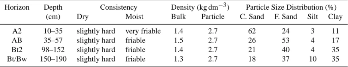
Table 1. Physical properties of selected horizons of Argissol, as per Melo and dos Santos (1996).
Horizon Depth Consistency Density (kg dm−3) Particle Size Distribution (%)
(cm) Dry Moist Bulk Particle C. Sand F. Sand Silt Clay
A2 10–35 slightly hard very friable 1.4 2.7 62 24 3 11
AB 35–57 slightly hard friable 1.5 2.7 26 53 4 17
Bt2 98–152 slightly hard friable 1.4 2.7 21 40 4 35
Bt/Bw 150–190 slightly hard friable 1.3 2.7 18 37 10 35
2002; Pierret et al., 2002; Anderson et al., 2003; Rachmant et al., 2005; Gibson et al., 2006). The principal benefits of CT techniques are: reducing the physical impact of sampling, providing three-dimensional (3-D) information and allowing rapid scanning to study sample dynamics in near real-time (Rasiah and Aylmore, 1998b). Because of these benefits, CT scanning has been used to extract fractal dimensions related to soil structure. Peyton et al. (1994) evaluated the fractal di-mension of macropore-scale density. Zeng et al. (1996) cal-culated fractal lacunarity in a silt loam soil. Several authors have dedicated their attention to the appropriate pore-solid CT threshold, before calculating mass fractal and surface fractal dimensions (Rogasik et al., 1999; Gantzer and An-derson, 2002; Perret et al., 2003; Rachmant et al., 2005). Re-cently, Gibson et al. (2006) compared three fractal analytical methods to quantify the heterogeneity within soil aggregates; in this work, the frequency distribution of pore and solid components was clearly dependent on thresholding, which could not be generalized.
As far as we know, they didn’t quantify this effect onDm
andD1. The aim of the present study is to evaluate the effect
of the image thresholding value as well as the cube size on the calculation of mass fractal dimension (Dm)and entropy
dimension (D1). To this end, soil images from four horizons,
obtained from a Brazilian Argissolo (Melo and dos Santos, 1996) were analyzed to obtain these fractal dimensions ap-plying four different thresholds.
2 Materials and methods
2.1 Soil studied
Intact soil samples were collected from four horizons of an Argissolo in the Brazilian Soil Classification (EMBRAPA SOLOS, 2006), or Ultisol (FAO Soil Classification), formed on the Tertiary Barreiras group of formations in Pernambuco state (Itapirema Experimental Station) presenting a hardset-ting behavior, found throughout the coastal tablelands of northeast Brazil. The natural vegetation of the region is trop-ical, coastal rainforest. Macromorphology and micromor-phology, mineralogy, as well as key physical and character-istics of this soil, have been studied, from a genetic
perspec-tive, by Melo and dos Santos (1996). Physical characteris-tics, of relevance to the current study, are provided in Table 1. 2.2 CT imaging and image pre-treatment
The intact soil samples were imaged using an EVS (now GE Medical. London Canada) MS-8 MicroCT scanner. Though some samples required paring to fit the 64 mm diameter imaging tubes, field orientation was maintained. Imaging pa-rameters were 155 keV and 25µA.
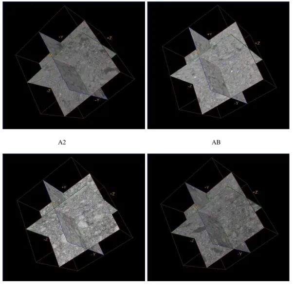
Proprietary software (GE Medical), was used to recon-struct the 16-bit, 3-D imagery from the sequence of axial views. The resulting voxel size was 45.1µm. File sizes ranged from 70 to 200 Mb, which made subsequent process-ing of the entire volume practically impossible. Accordprocess-ingly, one subvolume was extracted from each of the four origi-nal volumes (using GE Medical Microview); care was taken to ensure no edged effect of the subvolume. The subvol-umes measured 256×256×256 units, corresponding to about 16.8 million voxels. A 3-D Gaussian filter in MicroView (GE Healthcare, 2006) was also run on each sub-volume to reduce noise, typical of CT imagery. An example of a typical 3-D imagery is provided in Fig. 1.
2.3 Binary thresholding of CT imagery
A2 AB
Bt2 Bt/Bw
Fig. 1. Typical grey-scale CT imagery (orthogonal planes) of sub-volumes for each of the horizons studied. Dark regions correspond to less attenuating regions (pores), lighter areas to solid components. Z-axis is vertical, withZ+ representing top of sample. Length of edge of cube is 11.54 mm.
four threshold values were identified (Fig. 2): a) lower 3rd standard deviation of solid (low probability containing solid); b) central tendency for air (µCTair); c) equi-probability value
for air and solid and d) mean of the central tendencies for air and solid. Thresholds B and C are the most commonly used in soil science beside a subjective choice comparing the original and binary image by the experts, which we refuse to use in this study. Thresholds A and D were selected to have a total of four values to clearly study their influence on the fractal dimensions.
2.4 Mass fractal dimension
The binarized image is considered to represent two basic phases: pores and solid. Fractal analysis (FA) in 3-D
im-ages involves partitioning the space into cubes to construct samples and recording the number of cubes which cover the pores phase; this is repeated for different size cubes (Perret et al., 2003).
The cube-counting (CC), similar to the box-counting method in 2-D, combines voxels to form larger, mutually exclusive cubes each containing a different set of voxels. Given anL×L×L-voxel image, partitioned to a cube size ofδ×δ×δ, the number of cubes (n(δ))will follow the pro-portion of line sizeδ:
n(δ)∝
L
δ
3
884 A. M. Tarquis et al.: Influence of thresholding in fractal dimensions 0 1 2 3 4 5 6 7 8 9 10
-300 -275 -250 -225 -200 -17
CT values F re q u e n c y Air Solid B D C A µ µ µ
µCTair = µµµµCT
Fig. 2. Graphical representation of the different thresholding cri-teria, used to binarize the frequency distribution of CT values: A – CT value corresponding to 0.01% distribution of the CT values distribution of solid, B – mean of CT values of air (µCTair), C –
equi-probability CT values of air and solid and D – average of mean CT values of air (µCTair) and mean CT values of solid (µCTsolid).
one pixel belonging to the pore space (N (δ)) is recorded. BeingNj(δ)the number of cubes of sizeδwithj pixels
be-longing to the pore space (with a value from 1 toδ×δ×δ):
N (δ)= δ3
X
j=1
Nj(δ) (2)
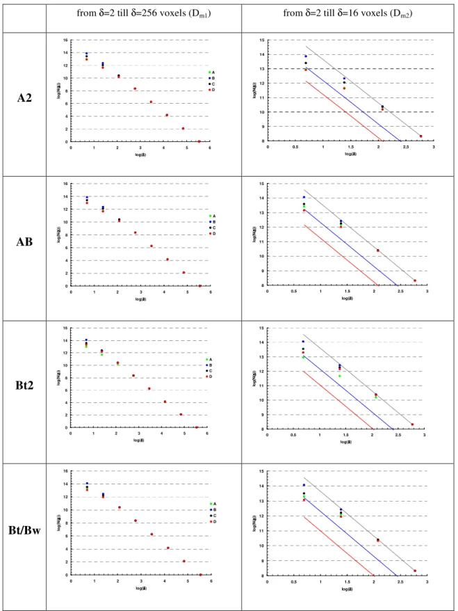
For a fractal set a log-log plot ofN (δ)vs.δgives:
N (δ)∝δ−Dm (3)
which yields a line of slope equal to−Dm; being Dm the
mass fractal dimension. It is expected that, as the object fills the space in 3-D,Dmwill approach the Euclidean dimension
(E)of three.
Given the relation (1) it is now instructive to seek bounds on the values the functionN (δ)can take based on Bird et al. (2006) work. We denote the fraction of the image occu-pied by pore phase at the finest resolution (i.e. porosity) byp. Ifp=1 the number of cubes required to cover the set is Lr2
and this is trivially an upper bound forN(δ) whenp<1. In order to derive a lower bound, we consider the situation in which the cubes cover the set but no part of the complemen-tary set. If this were to occur, then the number of cubes is equal to Lr2f. In general, the cubes will cover part of the complementary set and consequently the former number of cubes is a lower bound forN (δ). We may now write that N (δ)must satisfy the inequalities:
L
r
2
f ≤N (r)≤
L
r
2
(4) In terms of the log-log plot used to extract a mass fractal dimension, these inequalities result in two parallel reference
y = 0.0002x - 0.3336 R2 = 0.9074
y = 0.0002x - 0.9793 R2 = 0.9824
y = 0.0001x - 0.3642 R2 = 0.8858
y = 0.0002x - 0.227 R2 = 0.7248
5% 10% 15% 20% 25% 30% 35%
0 1000 2000 3000 4000 5000 6000
CT units p o ro s it y A2 AB Bt2 Bt/Bw
Fig. 3. Soil porosity versus CT units of threshold for each horizon and sub-volume. Linear fits for each horizon represents the change of porosity per CT unit.
lines of slope−3, between which the measured data must lie. The vertical spacing between these lines is equal to log(p). For all images sharing a common value ofp, the cube count-ing data will lie between these boundcount-ing lines. Analytically, we can conclude that the higher the porosity, the closer the boundary lines are and thenDmvalue will be closer to 3.
2.5 Entropy dimension
This calculation in 3-D imagery involves partitioning the space into cubes to construct samples with multiple scales. The cube-counting method (CC), similar to box-counting method in 2-D, combines voxels to form larger, mutually ex-clusive cubes each containing a different set of voxels. Given anL×L×L-voxel image, partitioned to a cube grid of size δ×δ×δ, the fraction of pore space (µi)in eachn(δ)cubes
(density) is calculated from: µi =
mi
mT
= mi
n(δ)
P
i=1
mi
(5)
wheremi is the number of pore class voxels in cubei, and
mT is the total number of pore class voxels in an image. In
this case, the pore density is the measure and the cube grid the support. When computing the number of cubes of size δ, the possible values of mi range from 0 to δ×δ×δ. So,
ifNj(δ)is the number of cubes containingj voxels of pore
volume in a given grid, Eqs. (4) and (5) can then be combined (Barnsley et al., 1988):
n(δ)
X
i=1
µi(δ)= n(δ)
X
i=1
m i mT = δ3 X
j=1
Nj(δ)
j
mT
(6)
where:mT= δ3
P
j=1
from δ=2 till δ=256 voxels (Dm1) from δ=2 till δ=16 voxels (Dm2)
A2
0 2 4 6 8 10 12 14 16
0 1 2 3 4 5 6
log(δδδδ)
lo
g
(N
(δδδδ
))
A B C D
8 9 10 11 12 13 14 15
0 0.5 1 1.5 2 2.5 3
log(δδδδ)
lo
g
(N
(δδδδ
))
AB
0 2 4 6 8 10 12 14 16
0 1 2 3 4 5 6
log(δδδδ)
lo
g
(N
(δδδδ
))
A B C D
8 9 10 11 12 13 14 15
0 0.5 1 1.5 2 2.5 3
log(δδδδ)
lo
g
(N
(δδδδ
))
Bt2
0 2 4 6 8 10 12 14 16
0 1 2 3 4 5 6
log(δδδδ)
lo
g
(N
(δδδδ
))
A B C D
8 9 10 11 12 13 14 15
0 0.5 1 1.5 2 2.5 3
log(δδδδ)
lo
g
(N
(δδδδ
))
Bt/Bw
0 2 4 6 8 10 12 14 16
0 1 2 3 4 5 6
log(δδδδ)
lo
g
(N
(δδδδ
))
A B C D
8 9 10 11 12 13 14 15
0 0.5 1 1.5 2 2.5 3
log(δδδδ)
lo
g
(N
(δδδδ
))
886 A. M. Tarquis et al.: Influence of thresholding in fractal dimensions
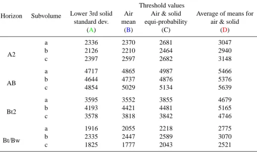
Table 2. Threshold values obtained applying different methods: A) CT value that represent the 0.1% of the CT values distribution corre-sponding to solid; B) average of CT values correcorre-sponding to air; C) intersection point of frequency distribution of CT values correcorre-sponding to air and solid and D) mean of average CT values corresponding to air and average CT values corresponding to solid.
Horizon Subvolume
Threshold values
Lower 3rd solid Air Air & solid Average of means for standard dev. mean equi-probability air & solid
(A) (B) (C) (D)
A2
a 2336 2370 2681 3047
b 2126 2210 2464 2940
c 2397 2597 2682 3148
AB
a 4717 4865 4987 5466
b 4644 4737 4876 5376
c 4854 5029 5134 5639
Bt2
a 3595 3552 3855 4679
b 4193 4421 4481 5165
c 3578 3818 3842 4746
Bt/Bw
a 1916 2055 2218 2775
b 2335 2447 2589 3070
c 1825 1777 2043 2521
By using the distribution functionNj(δ)it simplifies
cal-culations and reduces computational errors (Barnsley et al., 1988). The entropy of the system is estimated through this dimension by the relation (Feder, 1989):
D1= lim
δ→0
n(δ)
P
i=1
µi(δ)log [µi(δ)]
logδ =δlim→0
S(δ)
logδ (7)
The higher theD1is, the lower the information (higher
un-certainty) we have on the distribution of pore/solid fractions achieving a higher homogeneity. Contrary, the lower the val-ues ofD1, the more information (lower uncertainty) we have
on this distribution and then lower homogeneity.
The lower and upper limits of S(δ) were calculated in function of the porosity (p)for 3-D binary images given:
3 ln
L
δ
+ln(p) <− n(δ)
X
i=1
µiln(µi) <3 ln
L
δ
(8)
the bounding functions when included on the plot of entropy against ln(δ)again yield two parallel lines of slope 3, with separation of ln(p). The higher the porosity, the closer the two boundaries andD1will approach 3.
3 Results and discussion
3.1 Thresholding methods
As indicated in Table 2, the mean of the modal values for the air and solid distributions consistently resulted in the
largest thresholding values, followed by the equi-probability value for the two distributions. Though the thresholding val-ues corresponding to the other two criteria were consistently lower than those obtained from both distributions, there was no consistent trend between the air mean and the lower 3rd standard deviation of the solid distributions. A variation of specific thresholding values, among subvolumes of a given sample, suggests the high variability in the intensity field ob-tained from the CT scan. As indicated in Fig. 3, apparent porosity was more sensitive to the selected thresholding cri-teria in the Bt/Bw horizons than for the A2 and AB horizons, which followed a more linear trend. However, Bt/Bw is less sensitive to thresholding criteria than the Bt2 horizon. 3.2 Mass fractal dimension
For all horizons, the porosity obtained varied as a function of the threshold method applied (Table 3). As expected, thresh-old method D gave the higher porosity, from 24% for the A2 horizon to 28% for the AB horizon, and threshold method A gave the lowest, from 8% for the Bt/Bw horizon to 10% for the AB horizon. In all cases, we obtain statistically signif-icant straight-line fits (R2>0.98) for the full range of box sizes considered (from 1 to 256 voxels) as it is shown in Ta-ble 3 (Dm1). The mass fractal dimensions derived from these
calculations are very close to 3, with the lowest being 2.70 for A2 horizon using threshold method A, and the highest 2.94 for horizons AB, Bt2 and Bt/Bw, when applying method D. Comparing among horizons (Table 3), the A2 horizon always exhibited the lowest value inDmand Bt2 the highest value,
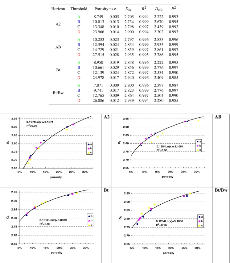
Table 3. Average (three replicates) porosity and mass dimension (Dm)for each horizon and thresholding criteria based on a range fromδ=2
tillδ=256 voxels (Dm1)and fromδ=2 tillδ=16 voxels (Dm2). For all linear fits theR2obtained was higher than 0.98.
Horizon Threshold Porosity±s.e. Dm1 R2 Dm2 R2
A2
A 8.749 0.003 2.703 0.994 2.222 0.993
B 10.013 0.013 2.734 0.999 2.670 0.995 C 13.348 0.010 2.798 0.997 2.439 0.992
D 23.966 0.014 2.900 0.994 2.202 0.993
AB
A 10.253 0.023 2.797 0.996 2.833 0.996
B 12.594 0.024 2.834 0.999 2.933 0.999 C 14.729 0.021 2.859 0.997 2.861 0.997
D 27.515 0.028 2.935 0.995 2.786 0.995
Bt
A 8.950 0.019 2.838 0.996 2.222 0.993
B 10.661 0.029 2.856 0.999 2.776 0.997 C 12.139 0.024 2.872 0.997 2.534 0.990
D 24.978 0.017 2.940 0.996 2.409 0.985
Bt/Bw
A 7.871 0.009 2.800 0.996 2.397 0.987
B 9.741 0.017 2.823 0.999 2.776 0.997 C 12.765 0.009 2.864 0.997 2.504 0.990
D 26.086 0.012 2.939 0.994 2.280 0.985
2.65 2.70 2.75 2.80 2.85 2.90 2.95
5% 10% 15% 20% 25% 30% porosity
D0 a
b
c
0.1971Ln(x)+3.1871 R2=0.98
A2
2.65 2.70 2.75 2.80 2.85 2.90 2.95
5% 10% 15% 20% 25% 30% porosity
D0 a
b
c
0.1284Ln(x)+3.1081 R2
=0.98
AB
2.65 2.70 2.75 2.80 2.85 2.90 2.95
5% 10% 15% 20% 25% 30% porosity
D0 a
b
c
0.1012Ln(x)+3.0839 R2=0.99
Bt
2.65 2.70 2.75 2.80 2.85 2.90 2.95
5% 10% 15% 20% 25% 30% porosity
D0 a
b
c
0.1204Ln(x)+3.1058 R2=0.96
Bt/Bw
Fig. 5. Mass fractal dimension (Dm)versus porosity for each horizon and sub-voxel. Logarithmic regression lines and their corresponding
888 A. M. Tarquis et al.: Influence of thresholding in fractal dimensions
2.51 2.56 2.61 2.66 2.71 2.76 2.81 2.86 2.91
5% 10% 15% 20% 25% 30% porosity
D1
a
b
c
0.2319Ln(x)+3.1484 R2=0.99
A2
2.51 2.56 2.61 2.66 2.71 2.76 2.81 2.86 2.91
5% 10% 15% 20% 25% 30% porosity
D1
a
b
c
0.1769Ln(x)+3.1089 R2=0.98
AB
2.51 2.56 2.61 2.66 2.71 2.76 2.81 2.86 2.91
5% 10% 15% 20% 25% 30% porosity
D1
a
b
c
0.1278Ln(x)+3.0682 R2=0.97
Bt
2.51 2.56 2.61 2.66 2.71 2.76 2.81 2.86 2.91
5% 10% 15% 20% 25% 30% porosity
D1 a
b
c
0.1629Ln(x)+3.1006 R2=0.96
Bt/Bw
Fig. 6. Entropy fractal dimension (D1)versus porosity for each horizon and sub-voxel. Logarithmic regression lines and their corresponding
equation are included in each graphic.
In order to closely examine the relationship between porosity and mass fractal dimension, a bi log plot of N(δ)and δis shown in more detail (Fig. 4). It is now apparent that soil porosity is mainly affecting the smallest voxels from length sizeδ=2 to 16 that influence theDm value obtained. If we
reduce our estimation ofDmto this size range (Dm2)values
are lower and show more variation (Table 3). From now on, we will use onlyDm1and named it asDm.
At the highest porosity values (Table 3), the differences in Dmamong the horizons are much smaller than at the lowest
values. Moreover, it was observed that, for each horizon, the trend was not linear, but rather showed several increments that can be fitted by a logarithmic curve. To study this obser-vation closer, several plots were done to see the variation of Dmversus porosity for each horizon and sub-voxel (Fig. 5).
What can easily be seen is that for a certain horizon it didn’t matter what the porosity for each sub-voxel and threshold was, all of them follow a pattern. This pattern is different de-pending on the horizon. In the case of the horizon AB, sub-voxelcis different from the other two, highlighting a possi-ble propossi-blem in the image due to a beam hardening effect that
was verified. For this reason, we didn’t include sub/voxelc in the logarithmic regression for this horizon.
Comparing these results to the particle size distribution (PSD) and depth for each horizon (Table 1), it can be ob-served that the most superficial one (A2) and with higher coarse sand percentage (62%) presents the steepest curve with respect to porosity (Fig. 5). Next horizon, AB, reduces the curve convexity as it shows a reduction to 26% of coarse sand and its depth (lower than 35 cm) protect it from any tillage practice. With the last two horizons, the clay per-centage increases to double (35%) and has a low percent-age in coarse sand. The curves of D0 versus porosity are
quite close and show the lower coefficients values multiply-ing Ln(porosity).
3.3 Entropy and correlation dimension
After calculating S(δ)for all binary images, it was plotted against log(δ); a clear linear pattern was observed in all plots (data not shown). The same comments that we have made forDmcould be applied here too. Table 4 shows the results
2.65 2.70 2.75 2.80 2.85 2.90 2.95
5% 10% 15% 20% 25% 30%
porosity
D
0
A2
AB
Bt2
Bt/Bw
2.55 2.60 2.65 2.70 2.75 2.80 2.85 2.90
5% 10% 15% 20% 25% 30%
porosity
D
1
A2
AB
Bt2
Bt/Bw
Fig. 7. Mass fractal dimension (Dm)and entropy fractal dimension
(D1)versus porosity for each horizon. Horizon AB is represented
only by sub-voxelsaandb.
The higher the threshold value (from A to D), the higher the porosity andD1increases approaching the value of 3 and the
s.e. decreases. At threshold D allD1are higher than 2.90,
pointing out a high homogeneity. As we did for mass di-mension, we plottedD1 for each horizon versus the
poros-ity of the soil at that threshold value (Fig. 6) realizing again that each sub-voxel differs in the porosity andD1associated,
the three of them variesD1 similarly when the threshold is
pushed forward. For example, this trend for horizon A2 is much more linear forD1 case than forDm values. At the
same time, AB shows a big difference in sub-voxelc with respect to sub-voxelaandb.
Once these fractal dimensions versus porosity have been analyzed, all the horizons are plotted together forD1 and
Dm(Fig. 7). In both it is clear that A2 shows a very
distinc-tive trend more than the other three horizons pointing out the influence of a high percentage of coarse sand and being the most superficial horizon that can be affected by tillage
prac-Table 4. Entropy dimension (D1), average of each horizon based
on the three replicates applying four different threshold values.
Horizon Threshold D1±s.e.
A2
A 2.699 0.033
B 2.739 0.036 C 2.809 0.021
D 2.910 0.011
AB
A 2.876 0.076
B 2.904 0.060 C 2.920 0.051
D 2.969 0.016
Bt2
A 2.915 0.013
B 2.921 0.016 C 2.929 0.007
D 2.958 0.003
Bt/Bw
A 2.846 0.057
B 2.859 0.066 C 2.898 0.037
D 2.957 0.015
tices. Horizon Bt2 shows the minimum slope in variations of DmandD1versus the porosity and therefore, versus
thresh-old, similarly with low content in coarse sand, low content in silt and 35% in clay. AB and Bt/Bw are inside the area marked by the other two horizons. Bt/Bw has the lowest con-tent in coarse sand (18%), a higher concon-tent in clay (35%) as Bt2 but higher content in silt compared with the rest of the horizons (10%).
4 Conclusions
3-D CT images from undisturbed soil samples were obtained from four horizons and three adjacent positions, having a to-tal set of 12 samples. In order to describe the porosity struc-ture, four threshold values were applied to convert each im-age into binary and then calculateDmandD1as a
quantifi-cation of soil morphology.
The sensitivity of each horizon to the threshold value on porosity was revealed indicating the differences in the CT unit values histogram among horizons although with these types of analyses, results cannot reflect the space arrange-ment of pores.
Linear scaling was observed over all the cube sizes for both fractal dimensions, however depending on the range of cube sizes used in the linear regression, the values obtained changed. For example, in one of the imagesDmcould vary
890 A. M. Tarquis et al.: Influence of thresholding in fractal dimensions
DmandD1showed a logarithmic relation with the
appar-ent porosity in the image for the 12 samples studied. Plotting all the data of porosity and itsDmorD1independently of the
threshold applied, the increase of both with respect to poros-ity defining a characteristic feature for each horizon that indi-rectly differentiate their structures. These differences can be explained based on the texture and depth of each horizon. TheseDm variations are in agreement with the functional
box-counting concept presented by Lovejoy et al. (1987) to extract the multiple dimensions of multiscale fields. Further research is necessary to present a wider variability in soil tex-ture and applying this type of analysis so a statistical analysis can be made in order to estimate these relationships. How-ever, from these results we can conclude that the higher the porosity, the harder it is to differentiate the differences inDm
andD1among horizons.
This indicates that fractal/multifractal analysis of the CT unit values could be applied to be able to choose an opti-mal thresholding as it is already used in many areas of geo-science.
Acknowledgements. Second author acknowledges the Canadian
Foundation for Innovation and Ontario Innovation Trust for providing funding to acquire the micro-CT scanning system, as well as EVS (now GE Medical) of London, Canada for designating micro-CT laboratory as Luminary Site. The funding of Madrid Au-tonomous Community (CM) under projects number M070020163 and M0800204139 is greatly appreciated.
Edited by: Q. Cheng
Reviewed by: X. Deyi, K. Oleschko, and two other anonymous referees
References
Anderson, S. H., Gantzer, C. J., Boone, J. M., and Tully, R. J.: Rapid nondestructive bulk density and soil-water content determination by computed tomography, Soil. Sci. Soc. A. J., 52, 35–40, 1988. Anderson, A. N., McBratney, A. B., and FitzPatrick, E. A.: Soil Mass, Surface, and Spectral Fractal Dimensions Estimated from Thin Section Photographs, Soil. Sci. Soc. A. J., 60, 962–969, 1996.
Anderson, S. H., Wang, H., Peyton, R. L., and Gantzer, C. J.: Es-timation of porosity and hydraulic conductivity from x-ray CT-measured solute breakthrough, in: Applications of X-ray Com-puted Tomography in the Geosciences, edited by: Mees, F., Swennen, R., Van Geet, M., and Jacobs, P., p. 135–149, Geo-logical Society of London Spec. Pub. 215, GeoGeo-logical Society of London, London, 2003.
Barnsley, M. F., Devaney, R. L., Mandelbrot, B. B., Peitgen, H. O., Saupe, D., and Voss, R. F.: The Science of Fractal Images, edited by: Peitgen, H. O. and Saupe, D., Springer-Verlag, New York, 66–67, 1988.
Bartoli, F., Bird, N. R., Gomendy, V., Vivier, H., and Niquet, S.: The relation between silty soil structures and their mercury porosime-try curve counterparts: fractals and percolation, Eur. J. Soil Sci., 50, 9–22, 1999.
Baveye, P., Boast, C. W., Ogawa, S., Parlange, J. Y., and Steen-huis, T.: Influence of image resolution and thresholding on the apparent mass fractal characteristics of preferential flow patterns in field soils, Water Resour. Res., 34, 2783–2796, 1998. Bird, N., D´ıaz, M. C., Saa, A., and Tarquis, A. M.: A Review of
Fractal and Multifractal Analysis of Soil Pore-Scale Images, J. Hydrol., 322, 211–219, 2006.
Brakensiek, D. L., Rawls, W. J., Logsdon, S. D., and Edwards, W. M.: Fractal description of macroporosity, Soil Sci. Soc. Am. J., 56, 1721–1723, 1992.
Buczhowski, S., Hildgen, P., and Cartilier, L.: Measurements of fractal dimension by box-counting: a critical analysis of data scatter, Physica A, 252, 23–24, 1998.
Crawford, J. W. and Matsui, N.: Heterogeneity of the pore and solid volume of soil: distinguishing a fractal space from its non-fractal complement, Geoderma, 73, 183–195, 1996.
Crawford, J. W., Baveye, P., Grindrod, P., and Rappoldt, C.: Ap-plication of Fractals to Soil Properties, Landscape Patterns, and Solute Transport in Porous Media, in: Assessment of Non-Point Source Pollution in the Vadose Zone, Geophysical Monograph, 108, edited by: Corwin, D. L., Loague, K., and Ellsworth, T. R., American Geophysical Union, Wahington, D.C., p. 151, 1999. Crawford, J. W., Matsui, N., and Young, I. M.: The relation between
the moisture-release curve and the structure of soil, European J. of Soil Sci., 46, 369–375, 1995.
Dathe, A., Eins, S., Niemeyer, J., and Gerold, G.: The surface frac-tal dimension of the soil-pore interface as measured by image analysis, Geoderma, 103, 203–229, 2001.
Dathe, A. and Thulner, M.: The relationship between fractal prop-erties of solid matrix and pore space in porous media, Geoderma, 129, 279–290, 2005.
Elliot, T. R. and Heck, R. J.: A comparison of 2D and 3D thresh-olding of CT imagery, Can. J. Soil Sci., 87(4), 405–412, 2007. EMBRAPA SOLOS: Sistema de Clasificaˇcao de Solos, 2a Ediˇcao,
Empresa Brasileira de Pesquisa Agropecuaria, Solos, Rio de Janeiro, 306 pp, 2006.
Feder, J.: Fractals, Plenum Press, New York, p. 83–84, 1989. Gantzer, C. J. and Anderson, S. H.: Computed tomographic
measurement of macroporosity in chisel-disk and no-tillage seedbeds, Soil Tillage Res., 64, 101–111, 2002.
GE Healthcare: MicroView 2.1.2 – MicroCT Visualization and Analysis, London, Canada, pp 315, 2006.
Gibson, J. R., Lin, H., and Bruns, M. A.: A comparison of frac-tal analytical methods on 2- and 3-dimensional computed tomo-graphic scans of soil aggregates, Geoderma, 134, 335–348, 2006. Gim´enez, D., Allmaras, R. R., Huggins, D. R., and Nater, E. A.: Mass, surface and fragmentation fractal dimensions of soil frag-ments produced by tillage, Geoderma, 86, 261–278, 1998. Gim´enez, D., Allmaras, R. R., Nater, E. A., and Huggins, D.
R.:. Fractal dimensions for volume and surface of interaggregate pores – scale effects, Geoderma, 77, 19–38, 1997.
Grevers, M. C. J. and de Jong, E.: Evaluation of soil-pore continuity using geostatistical analysis on macroporosity in serial sections obtained by computed tomography scanning, in: Tomography of soil-water-root processes, edited by: Anderson, S. H. and Hop-mans, J. W., p. 73–86, SSSA Spec. Bub., 36, SSSA, Madison, WI, 1994.
Melo, F. J. R. and dos Santos, M. C.: Micromorfologia e mineralo-gia de dois solos de Tabuleiro costeiro de Pernambuco, R. bras. Ci. Solo, 20, 99–108, 1996.
Oleschko, K.: Delesse principle and statistical fractal sets: 1. Di-mensional equivalents, Soil Tillage Res., 49, 255–266, 1998. Oleschko, K., Fuentes, C., Brambila, F., and Alvarez, R.: Linear
fractal analysis of three Mexican soils in different management systems, Soil Technol., 10, 207–223, 1997.
Oleschko, K., Brambila, F., Aceff, F., and Mora, L. P.: From fractal analysis along a line to fractals on the plane, Soil Tillage Res., 45, 389–406, 1998.
Origin Lab Corporation: Origin Pro 7.5, Northampton, MA, pp 257, 2006.
Pachepsky, Y. A., Yakovchenko, V., Rabenhorst, M. C., Pooley, C., and Sikora, L. J.: Fractal parameters of pore surfaces as derived from micromorphological data: effect of long term management practices, Geoderma, 74, 305–319, 1996.
Perret, J. S., Prasher, S. O., Kantzas, A., and Langford, C.: 3D visualization of soil macroporosity using X-ray CAT scanning, Can. Agric. Eng. J., 39, 249–261, 1997.
Perret, J. S., Prasher, S. O., Kantzas, A., and Langford, C.: Charac-terization of macropore morphology in a sandy loam soil using X-ray computer assisted tomography and geostatistical analysis, Can. Water Resou. J., 23, 143–166, 1998.
Perret, J., Prasher, S. O., Kantzas, A., and Langford, C.: Three-Dimensional Quantification of Macropore Networks in Undis-turbed Soil Cores, Soil Sci. Soc. Am. J., 63, 1530–1543, 1999. Perret, J. S., Prasher, S. O., and Kacimov, A. R.: Mass fractal
di-mension of soil macropores using computed tomography: from box-counting to the cube-counting algorithm, European J. Soil Sci., 54, 569–579, 2003.
Perrier, E., Tarquis, A. M., and Dathe, A.: A Program for Fractal and Multifractal Analysis of Two-Dimensional Binary Images. Computer Algorithms versus Mathematical Theory, Geoderma, 134, 284–294, 2006.
Peyton, R. L., Gantzer, C. J., Anderson, S. H., Haeffner, B. A., and Pfeifer, P.: Fractal dimension to describe soil macropore struc-ture using X ray computed tomography, Water Resour. Res., 30, 691–700, 1994.
construction and quantification of macropores using X-ray com-puted tomography and image analysis, Geoderma, 106, 247–271, 2002.
Rasband, W.: ImageJ 1.36, National Insitutes of Health, USA, 153 pp, 2006.
Rasiah, V. and Aylmore, L. A. G.: Estimating microscale spatial distribution of conductivity and pore continuity using computed tomography, Soil Sci. Soc. Am. J., 62, 1197–1202, 1998a. Rasiah, V. and Aylmore, L. A. G.: Characterizing the changes in soil
porosity by computed tomography and fractal dimension, Soil Sci., 163, 203–211, 1998b.
Rachman, A., Anderson, S. H., and Gantzer, C. J.: Computed-Tomographic Measurement of Soil Macroporosity Paramenters as Affected by Staff-Stemmed Grass Hedges, Soil Sci. Soc. Am. J., 69, 1609–1616, 2005.
Rogasik, H., Crawford, J. W., Wendroth, O., Young, I. M., Joshko, M., and Ritz, K.: Discrimination of soil phases by dual energy X-ray tomography, Soil Sci. Soc. Am. J., 63, 741–751, 1999. Saucier, A.: Effective permeability of multifractal porous media,
Physica A, 183, 381–397, 1992.
Tarquis, A. M., Gim´enez, D., Saa, A., D´ıaz, M. C., and Gasc´o, J. M.: Scaling and Multiscaling of Soil Pore Systems Determined by Image Analysis, in: Scaling Methods in Soil Physics, edited by: Pachepsky, Y. A., Radcliffe, D. E., and Selim, H. M. E., CRC Press, 434 pp, 2003.
Tel, T. and Vicsek, T.: Geometrical multifractality of growing struc-tures, J. Phys. A, General, 20, L835–L840, 1987.
Warner, G. S., Nieber, J. L., Moore, I. D., and Geise, R. A.: Char-acterizing macropores in soil by computed tomography, Soil Sci. Soc. Am. J., 53, 653–660, 1989.