JHEP05(2013)090
Published for SISSA by SpringerReceived: March 20, 2013
Accepted: April 30, 2013
Published:May 17, 2013
Studies of jet mass in dijet and W/Z + jet events
The CMS collaboration
E-mail: [email protected]
Abstract:Invariant mass spectra for jets reconstructed using the anti-kTand
Cambridge-Aachen algorithms are studied for different jet “grooming” techniques in data corresponding to an integrated luminosity of 5 fb−1, recorded with the CMS detector in proton-proton collisions at the LHC at a center-of-mass energy of 7 TeV. Leading-order QCD predictions for inclusive dijet and W/Z+jet production combined with parton-shower Monte Carlo models are found to agree overall with the data, and the agreement improves with the implementation of jet grooming methods used to distinguish merged jets of large transverse momentum from softer QCD gluon radiation.
JHEP05(2013)090
Contents
1 Introduction 1
2 Jet clustering algorithms and grooming techniques 3
2.1 Sequential jet clustering algorithms 3
2.2 Filtering algorithm 4
2.3 Trimming algorithm 5
2.4 Pruning algorithm 5
2.5 Groomed jet mass 5
3 The CMS detector and simulation 6
4 Triggers and event reconstruction 7
4.1 Dijet trigger selection 7
4.2 V+jet trigger selection 8
4.3 Binning jets as a function of pT 9
4.4 Event reconstruction 9
5 Event selection 10
6 Influence of pileup on jet grooming algorithms 11
7 Corrections and systematic uncertainties 13
8 Results from dijet final states 15
9 Results from V+jet final states 15
10 Summary 28
The CMS collaboration 33
1 Introduction
The variables most often used in analyses of jet production are jet directions and trans-verse momenta (pT). However, as jets are composite objects, their invariant masses (mJ)
JHEP05(2013)090
evolved jets can be used to discriminate them from lighter objects generated inquantum-chromodynamic (QCD) radiative processes. The same argument also holds for any new massive particles produced at the LHC. For sufficiently large boosts, all the decay products tend to be emitted as collimated groupings into small sections of the detector, and the re-sulting particles can be clustered into a single jet. Jet “grooming” techniques are designed to separate such merged jets from background. These new techniques have been found to be very promising for identifying decays of highly-boosted W bosons and top quarks, and in searches for Higgs bosons and other massive particles [1]. The main advantage of these grooming techniques is their ability to distinguish high pT jets that arise from decays of massive, possibly new, particles. In addition, their robust performance is valuable in the presence of additional interactions in an event (pileup), which is likely to provide an even greater challenge to such analyses in future higher-luminosity runs at the LHC.
Only a few of these promising approaches have been studied in data at the Tevatron [2] or at the LHC [3]. To understand these techniques in the context of searches for new phenomena, the jet mass must be well-modeled through leading-order (LO) or next-to-leading-order (NLO) Monte Carlo (MC) simulations. Much recent theoretical work in QCD has focused on the computation of jet mass, including predictions using advances in an effective field theory of jets (soft collinear effective theory, SCET) [4–23]. Studies of the kind reported in the present analysis can provide an understanding of the extent to which MC simulations that match matrix-element partons with parton showers can model the observed internal jet structure. Results of these studies can also be used to compare data with theoretical computations of jet mass, and to provide benchmarks for the use of these algorithms in searches for highly-boosted Higgs bosons, or new objects beyond the SM, especially by investigating some of the background processes expected in such analyses.
We present a measurement of jet mass in a sample of dijet events, and the first study of such distributions in V+jet events, where V refers to a W or Z boson. The data cor-respond to an integrated luminosity of 5.0 ±0.2 fb−1, collected by the Compact Muon Solenoid (CMS) experiment at the LHC in pp interactions at a center-of-mass energy of 7 TeV. The analysis of these two types of final states provides complementary information because of their different parton-flavor content, since the selected dijet events are domi-nated by gluon-initiated jets, and the V+jet events often contain quark-initiated jets. We focus on measuring the jet mass after applying several jet grooming techniques involving “filtering” [24], “trimming” [25], and “pruning” [26,27] of jets, as discussed in detail below. This work also presents the first attempt to measure the mass of trimmed and pruned jets. To study the dependence of the differential distributions in mJ on jet pT, we measure
the distributions in intervals of jet transverse momentum. Formally, this can be expressed in terms of a double-differential cross section for jet production (d2σ/dp
TdmJ) that is
examined as a function of mJ for several nonoverlapping intervals in pT:
σ= Z
mJ Z
pT
d2σ(m
J, pT)
dmJdpT
dpTdmJ =
X
i
Z
mJ
dσi(mJ)
dmJ
dmJ =
X
i
σi, (1.1)
wherei= 1,2,3, . . .refers to the ith interval inpT, and the sum of contributions over all i is equal to the total observed cross sectionP
JHEP05(2013)090
as a function ofmJ for each pT interval can therefore be written asρi(mJ) =
1
σi ×
dσi
dmJ
, with Z
ρi(mJ) dmJ = 1. (1.2)
The distributions in reconstructed jet mass of eq. (1.2) include corrections used to unfold jets to the “particle” level; thepT intervals are defined for ungroomed jets, following energy corrections for the response of the detector.
For the dijet analysis, pT and mJ correspond to the average transverse momentum
and average jet mass of the two leading jets (i.e., of highest pT): pAVG
T = (pT1+pT2)/2 andmAVG
J = (mJ1+mJ2)/2. For the V+jet analysis, we use themJ andpT of the leading jet. Both quantities depend on the nature of the jet grooming algorithm, as discussed in section 2.
This paper is organized as follows. To introduce the subject, we first discuss jet clus-tering algorithms in section 2, focusing mainly on grooming techniques. After a brief description of the CMS detector and the MC samples in section3, we provide information pertaining to the collected data and a description of event reconstruction in section 4. Selection of events is then described in section 5, and the effect of pileup on jet mass is investigated in section6. This is followed in section7by the correction and unfolding proce-dures that are applied to themJ spectra and their corresponding systematic uncertainties.
In sections 8 and 9, we present the results of the dijet and V+jet analyses, respectively. Finally, observations and remarks on the presented results are summarized in section 10.
The distributions shown are also stored in HEPData format [28].
2 Jet clustering algorithms and grooming techniques
2.1 Sequential jet clustering algorithms
Jets are defined through sequential, iterative jet clustering algorithms that combine four-vectors of input pairs of particles until certain criteria are satisfied and jets are formed. For the jet algorithms considered in this paper, for each pair of particlesiand j, a “distance” metric between the two particles (dij), and the so-called “beam distance” for each particle
(diB), are computed:
dij = min(pT2in, pTj2n)∆R2ij/R2 (2.1)
diB =pT2in, (2.2)
wherepTiandpTjare the transverse momenta of particlesiandj, respectively, “min” refers
to the lesser of the twopTvalues, the integerndepends on the specific jet algorithm, ∆Rij =
p
(∆yij)2+ (∆φij)2 is the distance betweeniandj in rapidity (y= 12ln(E+pz)/(E−pz)) and azimuth (φ), andRis the “size” parameter of order unity [29], with all angles expressed in radians. The particle pair (i, j) with smallest dij is combined into a single object. All
distances are recalculated using the new object, and the procedure is repeated until, for a given objecti, all thedij are greater than diB. Object iis then classified as a jet and not
JHEP05(2013)090
The value for n in eqs. (2.1) and (2.2) governs the topological properties of the jets.Forn= 1 the procedure is referred to as thekT algorithm (KT). The KT jets tend to have irregular shapes and are especially useful for reconstructing jets of lower momentum [29]. For this reason, they are also sensitive to the presence of low-pTpileup (PU) contributions, and are used to compute the mean pT per unit area (in (y, φ)) of an event [30]. For
n = −1, the procedure is called the anti-kT (AK) algorithm, with features close to an idealized cone algorithm. The AK algorithm is used extensively in LHC experiments and by the theoretical community for finding well-separated jets [29]. Forn= 0, the procedure is called the Cambridge-Aachen (CA) algorithm. This relies only on angular information, and, like thekT algorithm, provides irregularly-shaped jets in (y, φ). The CA algorithm is useful in identifying jet substructure [31–33].
Jet grooming techniques [26] that reduce the impact of contributions from the under-lying event (UE), PU, and low-pT gluon radiation can be useful irrespective of the specific nature of analysis. These kinds of contributions to jets are typically soft and diffuse, and hence contribute energy to the jet proportional to the area [30]. Because grooming tech-niques reduce the areas of jets without affecting the core components, the resulting jets are less sensitive to contributions from UE and PU, while still reflecting the kinematics of the hard original process. We consider three forms of grooming, referred to as filtering, trimming, and pruning. Such techniques can be applied to jets clustered through different algorithms (KT, AK, or CA). For the dijet analysis, we choose to cluster jets with the
anti-kT algorithm with R = 0.7 (AK7), as these are used extensively at CMS. For the V+jet analysis, in addition to AK7 jets, we also study CA jets withR= 0.8 (CA8), considered in recent publications involving top-quark tagging [34], and withR= 1.2 (CA12), which was proposed for analyses involving highly-boosted objects [24]. After the initial jet clustering with AK7, CA8, or CA12, the constituents of those jets are reclustered with a (possibly different) jet algorithm (e.g., KT, CA, or AK), applying additional grooming conditions to the sequence of selection criteria used for clustering. The optimal choice of this secondary clustering algorithm depends on the grooming technique, as described below. For the tech-niques we have investigated, the parameters chosen for the algorithms correspond to those chosen by refs. [24–27], nevertheless specific optimization would appear to be advisable for all well-defined searches for new phenomena.
2.2 Filtering algorithm
The “mass-drop/filtering” procedure aims to identify symmetric splitting of jets of large
pT that have large mJ values. It was proposed initially for use in searches for the Higgs
boson [24], but we consider just the filtering aspects of this algorithm for grooming jets. For each jet obtained in the initial clustering procedure, the filtering algorithm defines a new, groomed jet through the following algorithm: (i) the constituents of each jet are reclustered using the CA algorithm withR = 0.3, thereby definingnnew subjetss1, . . . , sn,
JHEP05(2013)090
The new jet has fewer particles than the initial jet, thereby reducing the contributionfrom effects such as underlying event and pileup, and the new mJ and pT values are therefore smaller than those of the initial jet. As will be demonstrated in section2.5, with this choice of parameters, filtering removes the fewest jet constituents, and is therefore the least aggressive of the investigated jet grooming techniques.
2.3 Trimming algorithm
Trimming ignores particles within a jet that fall below a dynamic threshold in pT [25]. It reclusters the jet’s constituents using the kT algorithm with a radiusRsub, accepting only the subjets that have pTsub > fcutλhard, where fcut is a dimensionless cutoff parameter, and λhard is some hard QCD scale chosen to equal the pT of the original jet. The Rsub and fcutparameters of the algorithm are taken to be 0.2 and 0.03, respectively. As will be demonstrated, with this choice of parameters, trimming removes more jet constituents than the filtering procedure, but fewer jet constituents than pruning, and corresponds therefore to a moderately aggressive jet grooming technique.
2.4 Pruning algorithm
Following the clustering of jets using the original algorithm (either AK7, CA8, or CA12), the pruning algorithm [26,27] reclusters the constituents of the jet through the CA algo-rithm, using the same distance parameter, but additional conditions beyond those given in eq. (2.1). In particular, the softer of the two particlesiand j to be merged is removed when the following conditions are met:
zij =
min(pTi, pTj)
pTi+pTj
< zcut (2.3)
∆Rij > Dcut≡α·2
mJ
pT
, (2.4)
where mJ and pT are the mass and transverse momentum of the originally-clustered jet, and zcut and α are parameters of the algorithm, chosen to be 0.1 and 0.5, respectively. In our particular choice of parameters, we have chosen to divide the jet into two “exclusive” subjets (similarly to the exclusive kT algorithm [29], where one clusters constituents until the jets are all separated by the parameter R in eq. 2.1). As will be demonstrated, with this choice of parameters, pruning removes the largest number of jet constituents, and can therefore be regarded as the most aggressive jet grooming technique investigated. It was previously used in the CMS search for tt resonances [34].
2.5 Groomed jet mass
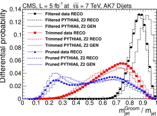
Figure 1 shows a comparison of distributions in the dijet sample for the ratio of groomed AK7 jet mass to the mass of the matched ungroomed AK7 jet, for our three grooming techniques, for data and forpythia6MC simulation [35], using the Z2 tune. Three
JHEP05(2013)090
jet
/ m
Groom jet
m
0
0.1 0.2 0.3 0.4 0.5 0.6 0.7 0.8 0.9
1
D
if
fe
re
n
ti
a
l
p
ro
b
a
b
ili
ty
0
0.02
0.04
0.06
0.08
0.1
0.12
0.14
Filtered data RECO
Filtered PYTHIA6, Z2 RECO Filtered PYTHIA6, Z2 GEN Trimmed data RECO
Trimmed PYTHIA6, Z2 RECO Trimmed PYTHIA6, Z2 GEN Pruned data RECO
Pruned PYTHIA6, Z2 RECO Pruned PYTHIA6, Z2 GEN Filtered data RECO
Filtered PYTHIA6, Z2 RECO Filtered PYTHIA6, Z2 GEN Trimmed data RECO
Trimmed PYTHIA6, Z2 RECO Trimmed PYTHIA6, Z2 GEN Pruned data RECO
Pruned PYTHIA6, Z2 RECO Pruned PYTHIA6, Z2 GEN Filtered data RECO
Filtered PYTHIA6, Z2 RECO Filtered PYTHIA6, Z2 GEN Trimmed data RECO
Trimmed PYTHIA6, Z2 RECO Trimmed PYTHIA6, Z2 GEN Pruned data RECO
Pruned PYTHIA6, Z2 RECO Pruned PYTHIA6, Z2 GEN
= 7 TeV, AK7 Dijets
s
at
-1
CMS, L = 5 fb
Figure 1. Distributions in differential probability for ratios of the jet mass of groomed jets to
their corresponding ungroomed values, for both dijet data andpythia6 (tune Z2) MC simulation, for the three grooming techniques discussed in the text: (i) filtering (circles, peaking near 0.9), (ii) trimming (squares, peaking near 0.75), and (iii) pruning (triangles, more dispersed).
particle-level jets frompythia6 (“PYTHIA GEN”). These three grooming techniques in-volve different jet algorithms for grooming (CA for filtering and pruning,kT for trimming) once the jets are found with AK7. The data and the simulation exhibit similar behavior. In general, the filtering algorithm is the least aggressive grooming technique, with groomed jet masses close to the ungroomed values. The trimming algorithm is moderately aggressive, and the pruning algorithm is the most aggressive of the three. With pruning, a bimodal distribution begins to appear, which is typical of our implementation of this algorithm as we require clustering into two exclusive subjets. In cases where the pruned jet mass is small, jets usually have most of their energy configured in “core” components, with little gluon radiation, which leads to narrow jets. When the pruned jet mass is large, the jets are split more symmetrically, which can be realized in events with gluons splitting into two nodes that fall within ∆R= 0.7 of the original parton.
3 The CMS detector and simulation
The CMS detector [36] is a general-purpose device with many features suited for recon-struction of energetic jets, specifically, the finely segmented electromagnetic and hadronic calorimeters and charged-particle tracking detectors.
JHEP05(2013)090
counterclockwise beam. The polar angleθ is measured relative to the positive z axis andthe azimuthal angle φrelative to thex axis in the x-y plane.
Charged particles are reconstructed in the inner silicon tracker, which is immersed in a 3.8 T axial magnetic field. The CMS tracking detector consists of an inner silicon pixel detector composed of three concentric central layers and two sets of disks arranged forward and backward of the center, and up to ten silicon strip central layers and three inner and nine outer strip disks forward and backward of the center. This arrangement provides full azimuthal coverage for |η|<2.5, where η =−ln[tan(θ/2)] is the pseudorapidity. The pseudorapidity approximates the rapidityyand equalsyfor massless particles. Since many of the reconstructed jets are not massless, we use the rapidity y for characterizing jets in this analysis.
A lead tungstate crystal electromagnetic calorimeter (ECAL) and a brass/scintillator hadronic calorimeter (HCAL) surround the tracking volume and provide photon, electron, and jet reconstruction up to |η|= 3. The ECAL and HCAL cells are grouped into tow-ers projecting radially outward from the center of the detector. In the central region (|η|<1.74), the towers have dimensions of ∆η = ∆φ= 0.087 that increase at larger |η|. ECAL and HCAL cell energies above some chosen noise-suppression thresholds are com-bined within each tower to define the tower energy. Muons are measured in gas-ionization detectors embedded in the steel return yoke outside the solenoid. To improve reconstruc-tion of jets, the tracking and calorimeter informareconstruc-tion is combined in a “particle-flow” (PF) algorithm [37], which is described in section4.4.
For the analysis of dijet events, samples are simulated with pythia6.4 (Tune Z2) [35,
38], pythia8(Tune 4c) [39], andherwig++(Tune 23) [40], and propagated through the
simulation of the CMS detector based onGeant4[41]. Underlying event (UE) and pileup
(PU) are included in the simulations, which are also reweighted to have the simulated PU distribution match the observed PU distribution in the data.
For the V+jet analysis, events with a vector boson produced in association with jets are simulated using MadGraph 5.1 [42]. This matrix element generator is also used to simulate tt events. The MadGraph events are subsequently subjected to parton shower-ing, simulated withpythia6using the Z2 Tune [38]. To compare hadronization in different
generators, we generate V+jet samples in which parton showering and hadronization are simulated with herwig++. Diboson (WW, WZ, and ZZ) events are also generated with
pythia6. Single-top-quark samples are produced with powheg [43], and the lepton
en-riched dijet samples are produced with pythia6 using the Z2 Tune. CTEQ6L1 [44] is the default set of parton distribution functions used in all these samples, except for the single-top-quark MC, which uses CTEQ6M.
4 Triggers and event reconstruction
4.1 Dijet trigger selection
trig-JHEP05(2013)090
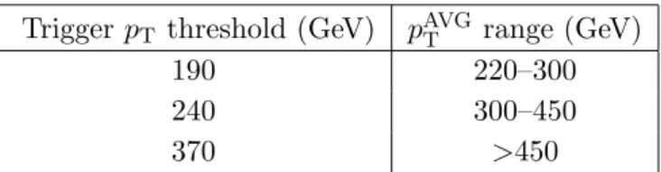
Trigger pT threshold (GeV) pAVGT range (GeV)190 220–300
240 300–450
370 >450
Table 1. TriggerpTthresholds for individual jets, and correspondingpAVGT intervals used to assign
the triggered events in the dijet analysis.
ger requirements. As the instantaneous luminosity is time-dependent, the specific jet-pT thresholds change with time. The triggers used to select dijet events have partial overlap. Those with lower-pT thresholds have high prescale settings to accommodate the higher data-acquisition rates, and some events selected with these lower-pT triggers are also col-lected at higher thresholds.
To avoid double counting of phase space, each event is assigned to a specific trigger. To do this, we compute the trigger efficiency as a function of reconstructed pAVG
T , select an interval in trigger efficiency where the efficiency is maximum (>95%) for that range of
pAVG
T , and assign that trigger to the appropriatep AVG
T interval. The assignment is based on the jetpT values reconstructed offline (but not groomed). Table1shows thepT thresholds for each of the jet triggers used in the analysis, and the corresponding intervals of pT to which the triggered events are assigned.
4.2 V+jet trigger selection
Several triggers are also used to collect events corresponding to the topology of V+jet events, where the V decays via electrons or muons in the final state. For the W+jet channels, the triggers consist of several single-lepton triggers, with lepton identification criteria applied online. To assure an acceptable event rate, leptons are required to be isolated from other tracks and energy depositions in the calorimeters. For the W(µνµ)
channel, the trigger thresholds for the muonpTare in the range of 17 to 40 GeV. The higher thresholds are used at higher instantaneous luminosity. The combined trigger efficiency for signal events that pass offline requirements (described in section5) is≈92%.
For the W(eνe) events, the electron pT threshold ranges from 25 to 65 GeV. To en-hance the fraction of W+jet events in the data, the single-electron triggers are also re-quired to have minimum thresholds on the magnitude of the imbalance in transverse en-ergy (Emiss
T ) and on the transverse mass (mT) of the (electron + E miss
T ) system, where
m2 T = 2E
e TE
miss
T (1−cosφ), andφis the angle between the directions ofp e
T andE miss T . The combined efficiency for electron W+jet events that pass the offline criteria is≈99%.
The Z(µµ) channel uses the same single-muon triggers as the W(µνµ) channel. The
JHEP05(2013)090
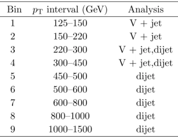
Bin pT interval (GeV) Analysis1 125–150 V + jet
2 150–220 V + jet
3 220–300 V + jet,dijet 4 300–450 V + jet,dijet
5 450–500 dijet
6 500–600 dijet
7 600–800 dijet
8 800–1000 dijet
9 1000–1500 dijet
Table 2. Intervals in ungroomed jetpTfor the V+jet and dijet analyses.
4.3 Binning jets as a function of pT
The jetpT bins introduced in eq. (1.1) are given in table2for V+jet and dijet events. The jet pT is re-evaluated for each grooming algorithm. Because there are large biases due to jet misassignment in the dijet events, especially at smallpT (when three particle-level jets are often reconstructed as two jets in the detector, or vice versa), thepT intervals for these events begin at 220 GeV. Furthermore, the smaller number of events in the V+jet samples precludes the study of these events beyondpT = 450 GeV.
4.4 Event reconstruction
As indicated above, events are reconstructed using the particle-flow algorithm, which com-bines the information from all subdetectors to reconstruct the particle candidates in an event. The algorithm categorizes particles into muons, electrons, photons, charged hadrons, and neutral hadrons. The resulting PF candidates are passed through each jet clustering algorithm of section 2, as implemented inFastJet (Version 3.0.1) [45,46].
The reconstructed interaction vertex characterized by the largest value of P
i(pTtrki )2, where pTtrki is the transverse momentum of the ith charged track associated with the ver-tex, is defined as the leading primary vertex (PV) of the event. This vertex is used as the reference vertex for all PF objects in the event. A pileup interaction can affect the recon-struction of jet momenta andEmiss
T , as well as lepton isolation and b-tagging efficiency. To mitigate these effects, a track-based algorithm is used to remove all charged hadrons that are not consistent with originating from the leading PV.
JHEP05(2013)090
are matched to signals in the muon chambers, and (ii) in which a global fit is performedto a track seeded by signals in the external muon system. The muon candidates are required to be reconstructed through both algorithms. Additional identification criteria are imposed on muon candidates to reduce the fraction of tracks misidentified as muons, and to reduce contamination from muon decays in flight. These criteria include the number of hits detected in the tracker and in the outer muon system, the quality of the fit to a muon track, and its consistency of originating from the leading PV.
Charged leptons from V-boson decays are expected to be isolated from other energy depositions in the event. For each lepton candidate, a cone with radius 0.3 for muons and 0.4 for electrons is chosen around the direction of the track at the event vertex. When the scalar sum of the transverse momenta of reconstructed particles within that cone, excluding the contribution from the lepton candidate, exceeds≈10% of thepTof the lepton candidate, that lepton is ignored. The exact isolation requirement depends on the η, pT, and flavor of the lepton. Muons and electrons are required to have pT > 30 GeV and > 80 GeV, respectively. The large threshold for electrons ensures good trigger efficiency. To avoid double counting, isolated charged leptons are removed from the list of PF objects that are clustered into jets.
After removal of isolated leptons and charged hadrons from pileup vertices, only the neutral hadron component from pileup remains and is included in the jet clustering. This remaining component of pileup to the jet energy is removed by applying a correction based on a mean pT per unit area of (∆y×∆φ) originating from neutral particles [30,49]. This quantity is computed using the kT algorithm, and corrects the jet energy by the amount of energy expected from pileup in the jet cone. This “active area” method adds a large number of soft “ghost” particles to the clustering sequence to determine the effective area subtended by each jet. This procedure is done for all grooming algorithms just as for the ungroomed jets. The active area of a groomed jet is smaller than that of an ungroomed jet, and the pileup correction is therefore also smaller. Different responses in the endcap and central barrel calorimeters necessitate using η-dependent jet corrections. The amount of energy expected from the remnants of the hard collision (the underlying event) is estimated from minimum-bias data and MC events, and is added back into the jet.
In addition, the pileup-subtracted jet four-momenta in data are corrected for nonlin-earities inηandpT by using apT- andη-dependent correction to account for the difference between the response in MC-simulated events and data [50]. The jet corrections are derived for the ungroomed jet algorithms but are also applied to the groomed algorithms, thereby adding additional systematic uncertainty in the energy of groomed jets.
5 Event selection
JHEP05(2013)090
Dijet events are required to have at least two AK7 jets, each with pT >50 GeV and|y|<2.5, and each jet must satisfy the jet quality criteria discussed in ref. [37]. No third-jet veto is applied.
Reconstruction of W and Z bosons in V+jet events begins with identification of charged leptons and a calculation of Emiss
T , described in the previous section. Candidates for Z →
ℓ+ℓ− (ℓ= e or µ) decays are reconstructed by combining two isolated electrons or muons
and requiring the dilepton invariant mass to be in the 80 < Mℓℓ < 100 GeV range. An
accurate measurement ofEmiss
T is essential for distinguishing the W signal from background processes. TheETmiss in the event is defined using the PF objects, and this analysis requires
Emiss
T >50 GeV. Candidate W→ℓνℓ decays are identified primarily through the presence
of a significant Emiss
T and a single isolated lepton of large pT, with pT and mT of the W candidate obtained by combining the lepton and theETmiss vectors.
The analysis of V+jet events is mainly of interest for the regime of pV
T >120 GeV, in which the opposing jet tends to have largepT as well, because of momentum conservation. In fact, the leading jet in each event (independent of clustering algorithm and jet radius) is required to have pT > 125 GeV and |y| < 2.5. A back-to-back topology between the vector boson and the leading jet is ensured by the additional selection of ∆φ(V, jet)> 2 and ∆R(ℓ,jet)>1. Requiring such highly boosted jets, in addition to the tight isolation criteria for the leptons, greatly suppresses the background from multijet production. In the W→ℓνℓ+jet analysis, additional rejection of multijet background is achieved by requiring
mT(W)>50 GeV. No subleading-jet veto is applied.
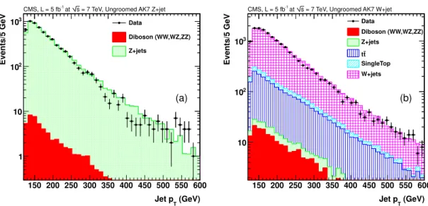
Figures 2(a) and (b) show the pT distributions for the leading AK7 jet selected in Z+jet and W+jet candidate events, respectively. Given the unique signature for highly-boosted vector bosons recoiling from jets, the selections suffice to define very pure samples of V+jet events. In the Z(ℓℓ)+jet analysis, the additional constraint on dilepton mass removes almost all background contributions, yielding a purity of ≈99% for Z+jet events, with≈1% contamination from diboson production. The W+jet candidate sample contains
≈82% W+jet events, with small background contributions from tt (13%), single top-quark (3%), and diboson and Z+jet (1% each) events based on MC simulation. The small number of events expected from these processes are subtracted using MC predictions for the jet mass from the W+jet candidate events, before correcting the data for detector effects. Similarly, the small number of events expected from diboson production are subtracted from the Z +jet candidates.
6 Influence of pileup on jet grooming algorithms
JHEP05(2013)090
(GeV)
T
Jet p 150 200 250 300 350 400 450 500 550 600
Events/5 GeV
1 10
2
10
3
10
(a)
Data
Diboson (WW,WZ,ZZ) Z+jets
= 7 TeV, Ungroomed AK7 Z+jet s
at
-1
CMS, L = 5 fb
(GeV)
T
Jet p 150 200 250 300 350 400 450 500 550 600
Events/5 GeV
10
2
10
3
10
(b)
Data
Diboson (WW,WZ,ZZ) Z+jets
t t SingleTop W+jets
= 7 TeV, Ungroomed AK7 W+jet s
at
-1
CMS, L = 5 fb
Figure 2. ThepTdistribution for the leading AK7 jet in accepted (a) Z+jet and (b) W+jet events.
Ratio of slopes Measured Expected
s0.7/s0.5 2.7±0.9 (stat.) (0.7/0.5)3 = 2.74
s0.8/s0.5 3.3±1.0 (stat.) (0.8/0.5)3 = 4.10
s0.8/s0.7 1.2±0.2 (stat.) (0.8/0.7)3 = 1.49
Table 3. Slopes of linear fits ofhmJias a function ofNPV for AK jets of differentR values.
of large angular extent that contain many particles. Grooming techniques are designed to reduce the effective area of such jets and thereby minimize sensitivity to pileup. We examine this issue through studies of jet mass in the presence of pileup.
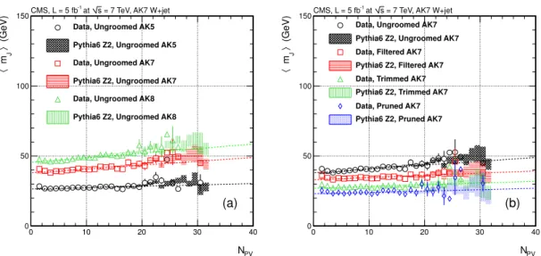
The mean jet mass hmJi for AK jets is presented for size parameters R = 0.5, 0.7,
and 0.8, as a function of the total number of reconstructed primary vertices (NPV) in figure 3(a), for data and MC simulation. The mean mass for NPV = 1 increases linearly with the jet radius from 0.5 to 0.8. A measure of the dependence of hmJi on pileup is
given by the slope of a linear fit to the jet mass versus NPV. The ratios of these slopes (sR) are found to be roughly consistent with the ratio of the third power of the jet radius,
as summarized in table3.
This is in agreement with predictions for scaling of the mean mass [51]. TheR3 dependence can be understood in terms of the increase of the jet area as R2. Simultaneously, the contribution of these particles to the jet mass scales with the distance between them, or
≈R/2, yielding another power ofR.
In figure 3(b) we show the dependence of hmJi on NPV, for AK7 jets, for different
grooming algorithms. The grooming significantly reduces the impact of pileup onhmJi, as
reflected by the decrease of the slope of the linear fit to the groomed-jet data points, as summarized in table4.
The observed agreement between data and simulation in figure 3provides support for our characterization of jet grooming and pileup, and the decrease in slopes suggests that grooming is indeed an effective tool for suppressing the impact of pileup on jets with large
JHEP05(2013)090
PV
N
0 10 20 30 40
(GeV)
〉
J
m
〈
0 50 100 150
Data, Ungroomed AK5 Pythia6 Z2, Ungroomed AK5 Data, Ungroomed AK7 Pythia6 Z2, Ungroomed AK7 Data, Ungroomed AK8 Pythia6 Z2, Ungroomed AK8
(a)
= 7 TeV, AK7 W+jet s
at
-1
CMS, L = 5 fb
PV
N
0 10 20 30 40
(GeV)
〉
J
m
〈
0 50 100 150
Data, Ungroomed AK7 Pythia6 Z2, Ungroomed AK7 Data, Filtered AK7 Pythia6 Z2, Filtered AK7 Data, Trimmed AK7 Pythia6 Z2, Trimmed AK7 Data, Pruned AK7 Pythia6 Z2, Pruned AK7
(b)
= 7 TeV, AK7 W+jet s
at
-1
CMS, L = 5 fb
Figure 3. Distributions of the average jet mass for AK jets as a function of the number of
reconstructed primary vertices: (a) for different jet radii, and (b) for AK7 jets, comparing the impact of grooming algorithms to results without grooming.
Jet R Clustering algorithm sR(GeV/PV)
AK5 ungroomed 0.10±0.03 (stat.) AK7 ungroomed 0.28±0.03 (stat.) AK7 filtered 0.16±0.02 (stat.) AK7 trimmed 0.12±0.04 (stat.) AK7 pruned 0.10±0.05 (stat.) AK8 ungroomed 0.33±0.03 (stat.)
Table 4. Values of slopes for the dependence ofhmJionNPV for AK jets with different radii and
clustering algorithms.
7 Corrections and systematic uncertainties
JHEP05(2013)090
Systematic uncertainties are estimated by modifying the response matrix for eachsource of uncertainty by ±1 standard deviation, and comparing the mass distribution to the nominal results, based on simulated pythia6 events. The difference in the unfolded mass spectrum from such a change is taken as the uncertainty arising from that source.
The experimental uncertainties that can affect the unfolding of the jet mass include the jet energy scale (JES), jet energy resolution (JER), and jet angular resolution (JAR). The uncertainty from JES is estimated by raising and lowering the jet four-momenta by the measured uncertainty as a function of jet pT and η [50], which typically corresponds to 1–2% for the jets in this analysis. Two additional pT- and η-independent uncertainties are included: a 1% uncertainty to account for differences observed between the measured and predicted W mass for high-pT jets in a tt-enriched sample, and a 3% uncertainty to account for differences in the groomed and ungroomed energy responses found in MC simulation [34].
The impact of uncertainties in JER and JAR on mJ are evaluated by smearing the
jet energies, as well as the resolutions in η and φ, each by 10% in the MC simulation relative to the particle-level generated jets [50]. These estimated uncertainties on JER and JAR are found to be essentially the same for all jet grooming techniques in MC studies. Since this analysis uses jets constructed from PF constituents, the charged particles have excellent energy and angular resolutions, but their use induces a dependence on tracking uncertainties, e.g., tracking efficiency. This dependence is accounted for implicitly in the
±10% changes in jet energy and angular resolutions, since such changes would lead to a difference between expected and observed values of these quantities. The same is true for the neutral electromagnetic component of the jet (primarily from π0
→γγ decays). The remaining sources of uncertainty are estimated from MC simulation. The tracking information is not sensitive to the neutral hadronic component of jets, and this small contribution is taken directly from simulation. We estimate this remaining uncertainty by comparing the unfolded data using pythia6 and using herwig++, and assign the
difference as a systematic uncertainty. This also accounts for the uncertainty from modeling parton showers. The latter effect often comprises the largest uncertainty in the unfolded jet mass distributions as described below. Other theoretical ambiguities that can affect the unfolding of the jet mass include the variation of the parton distribution functions and the modeling of initial and final-state radiation (ISR/FSR). The former was investigated and found to be much smaller than the difference between the unfolding withpythia6and the
unfolding withherwig++, and hence is neglected. The latter is included implicitly in the uncertainty betweenpythia6and herwig++.
As described in section 4.4, the jets used in this analysis are reconstructed after re-moving the charged hadrons that appear to emanate from subleading primary vertices. This procedure produces a dramatic (≈60%) reduction in the pileup contribution to jets. The residual uncertainty from pileup is obtained through MC simulation, estimated by increasing and decreasing the cross section for minimum-bias events by 8%.
JHEP05(2013)090
particle-level jets to reconstructed jets, and the magnitude of the bias correction is alsoadded to the overall systematic uncertainty. Such misassignments are negligible in the V+jet analysis.
8 Results from dijet final states
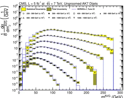
The differential probability distributions of eq. (1.2) for mAVG
J of the two leading jets in
dijet events, corrected for detector effects in the jet mass, are displayed in figures 4–7 for seven bins in pAVG
T along with the herwig++ predictions. The p AVG
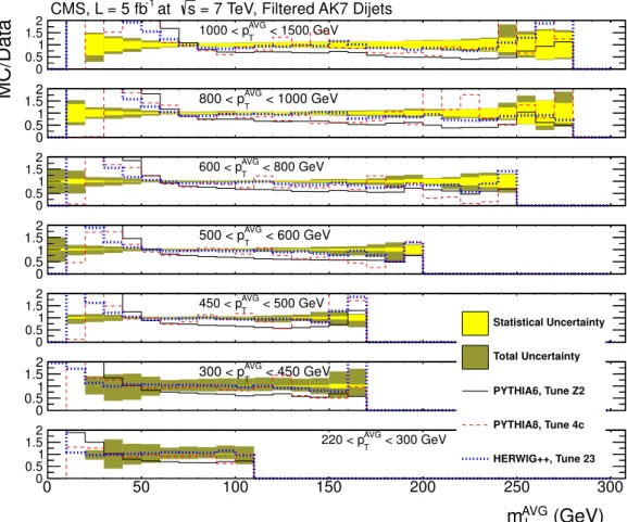
T is not corrected to the particle level, because the correction is expected to be negligible for the momenta considered. Results are shown for ungroomed jets and for the three categories of grooming. Each distribution is normalized to unity. The ratios of the MC simulations used in figures4– 7to the results for data, forpythia6,pythia8, and forherwig++are given in figures8–
11, respectively.
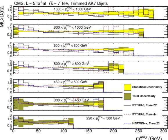
The largest systematic uncertainty is from the choice of parton-shower modeling used to calculate detector corrections, with small, but still significant uncertainties arising from jet energy scale and resolution, and small contributions from jet angular resolution and pileup. In the 220–300 GeV and 300–450 GeV jet-pT bins, the mJ < 50 GeV region is dominated
by uncertainties from unfolding (50–100%), which are negligible for pAVGT >450 GeV. For
mJ > 50 GeV, the JES, JER, JAR, and pileup uncertainties each contribute ≈10%. For
the 450–1000 GeVpT bins, parton showering dominates the uncertainties, which is around 50–100% below the peak of themJ distribution and 5–10% for the rest of the distribution.
ForpT>1000 GeV, statistical uncertainty dominates the entire mass range.
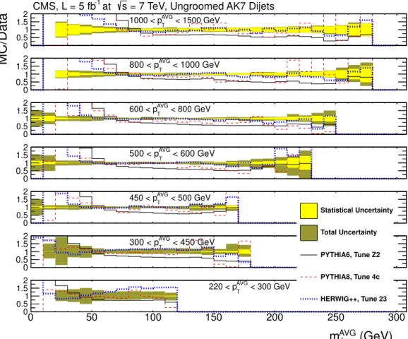
For clarity, the distributions in figures 8–11 are truncated where few events are recorded. Bins in mAVG
J with uncertainties of > 100% are ignored to avoid overlap with
more precise measurements in otherpAVG
T bins. The agreement withherwig++modeling of parton showers appears to be best for pAVGT >300 GeV and m
AVG
J >20 GeV. However,
the ungroomed and filtered jets show worse agreement for 20 < mAVG
J < 50 GeV when
pAVG
T > 450 GeV. For all generators and all p AVG
T bins, the agreement is better at larger jet masses. The disagreement is largest at the very lowest mass values, which correspond to the region most sensitive to the underlying event description and pileup, and where the amount of showering is apparently underestimated in the simulation.
9 Results from V+jet final states
This section provides the probability density distributions as functions of the mass of the leading jet in V+jet events. These distributions are corrected for detector effects in the jet mass, and are compared to MC expectations from MadGraph (interfaced to pythia6)
and herwig++. The jet mass distributions are studied in different ranges ofpT between
JHEP05(2013)090
(GeV)
AVG J
m
0 50 100 150 200 250 300
GeV 1 A V G J dm σ d σ 1 -6 10 -5 10 -4 10 -3 10 -2 10 -1 10 1 10 2 10 3 10 4 10 5 10 6 10 7 10 8
10 at s = 7 TeV, Ungroomed AK7 Dijets
-1
CMS, L = 5 fb
Statistical Uncertainty Total Uncertainty HERWIG++, Tune 23
) 0
220 - 300 GeV (x 10 1)
300 - 450 GeV (x 10 2)
450 - 500 GeV (x 10 3)
500 - 600 GeV (x 10
) 4
600 - 800 GeV (x 10 5)
800 - 1000 GeV (x 10 6)
1000 - 1500 GeV (x 10
Figure 4. Unfolded distributions for the mean mass of the two leading jets in dijet events for
reconstructed AK7 jets, separated according to intervals in pAVG
T (the mean pT of the two jets).
The data are shown by the symbols indicating different bins in the mean pT of the two jets.
The statistical uncertainty is shown in light shading, and the total uncertainty in dark shading. Predictions fromherwig++are given by the dotted lines. To enhance visibility, the distributions for larger values ofpAVG
T are scaled up by the factors given in the legend.
(GeV)
AVG J
m
0 50 100 150 200 250 300
GeV 1 A V G J dm σ d σ 1 -6 10 -5 10 -4 10 -3 10 -2 10 -1 10 1 10 2 10 3 10 4 10 5 10 6 10 7 10 8
10 at s = 7 TeV, Filtered AK7 Dijets
-1
CMS, L = 5 fb
Statistical Uncertainty Total Uncertainty HERWIG++, Tune 23
) 0
220 - 300 GeV (x 10 300 - 450 GeV (x 101) 450 - 500 GeV (x 102) 3)
500 - 600 GeV (x 10
) 4
600 - 800 GeV (x 10 5)
800 - 1000 GeV (x 10 6)
1000 - 1500 GeV (x 10
Figure 5. Unfolded distributions for the mean mass of the two leading jets in dijet events for
reconstructed filtered AK7 jets, separated according to intervals in pAVG
T (the meanpTof the two
jets). The data are shown by the symbols indicating different bins in the meanpT of the two jets.
The statistical uncertainty is shown in light shading, and the total uncertainty in dark shading. Predictions fromherwig++are given by the dotted lines. To enhance visibility, the distributions for larger values ofpAVG
JHEP05(2013)090
(GeV)
AVG J
m
0 50 100 150 200 250 300
GeV 1 A V G J dm σ d σ 1 -6 10 -5 10 -4 10 -3 10 -2 10 -1 10 1 10 2 10 3 10 4 10 5 10 6 10 7 10 8
10 at s = 7 TeV, Trimmed AK7 Dijets
-1
CMS, L = 5 fb
Statistical Uncertainty Total Uncertainty HERWIG++, Tune 23
) 0
220 - 300 GeV (x 10 1)
300 - 450 GeV (x 10 2)
450 - 500 GeV (x 10 3)
500 - 600 GeV (x 10
) 4
600 - 800 GeV (x 10 5)
800 - 1000 GeV (x 10 6)
1000 - 1500 GeV (x 10
Figure 6. Unfolded distributions for the mean mass of the two leading jets in dijet events for
reconstructed trimmed AK7 jets, separated according to intervals inpAVG
T (the meanpTof the two
jets). The data are shown by the symbols indicating different bins in the meanpT of the two jets.
The statistical uncertainty is shown in light shading, and the total uncertainty in dark shading. Predictions fromherwig++are given by the dotted lines. To enhance visibility, the distributions for larger values ofpAVG
T are scaled up by the factors given in the legend.
(GeV)
AVG J
m
0 50 100 150 200 250 300
GeV 1 A V G J dm σ d σ 1 -6 10 -5 10 -4 10 -3 10 -2 10 -1 10 1 10 2 10 3 10 4 10 5 10 6 10 7 10 8
10 at s = 7 TeV, Pruned AK7 Dijets
-1
CMS, L = 5 fb
Statistical Uncertainty Total Uncertainty HERWIG++, Tune 23
) 0
220 - 300 GeV (x 10 300 - 450 GeV (x 101) 450 - 500 GeV (x 102) 3)
500 - 600 GeV (x 10
) 4
600 - 800 GeV (x 10 5)
800 - 1000 GeV (x 10 6)
1000 - 1500 GeV (x 10
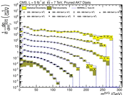
Figure 7. Unfolded distributions for the mean mass of the two leading jets in dijet events for
reconstructed pruned AK7 jets, separated according to intervals in pAVG
T (the meanpTof the two
jets). The data are shown by the symbols indicating different bins in the meanpT of the two jets.
The statistical uncertainty is shown in light shading, and the total uncertainty in dark shading. Predictions fromherwig++are given by the dotted lines. To enhance visibility, the distributions for larger values ofpAVG
JHEP05(2013)090
MC/Data
(GeV)
AVG J
m
0 0.5 1
1.52 AVG < 1500 GeV
T
1000 < p
0 0.51
1.52 AVG < 1000 GeV T
800 < p
0
0.51
1.52 AVG < 800 GeV
T
600 < p
0 0.51
1.52 500 < pAVGT < 600 GeV
0
0.51
1.52 AVG < 500 GeV
T
450 < p
0 0.51
1.52 300 < pAVGT < 450 GeV
0 50 100 150 200 250 300
0
0.51
1.52 220 < pAVGT < 300 GeV
Statistical Uncertainty
Total Uncertainty
PYTHIA6, Tune Z2
PYTHIA8, Tune 4c
HERWIG++, Tune 23 , Ungroomed AK7 Dijets
= 7 TeV s
at
-1
CMS, L = 5 fb
Figure 8. Ratio of MC simulation to unfolded distributions of the jet mass for AK7 jets for the
seven bins inpAVG
T . The statistical uncertainty is shown in light shading, and the total uncertainty
JHEP05(2013)090
MC/Data
(GeV)
AVG J
m
0 0.5 1
1.52 AVG < 1500 GeV
T
1000 < p
0 0.51
1.52 AVG < 1000 GeV T
800 < p
0
0.51
1.52 AVG < 800 GeV
T
600 < p
0 0.51
1.52 500 < pAVGT < 600 GeV
0
0.51
1.52 AVG < 500 GeV
T
450 < p
0 0.51
1.52 300 < pAVGT < 450 GeV
0 50 100 150 200 250 300
0
0.51
1.52 220 < pAVGT < 300 GeV
Statistical Uncertainty
Total Uncertainty
PYTHIA6, Tune Z2
PYTHIA8, Tune 4c
HERWIG++, Tune 23 , Filtered AK7 Dijets
= 7 TeV s
at
-1
CMS, L = 5 fb
Figure 9. Ratio of MC simulation to unfolded distributions of the jet mass for filtered AK7 jets
for the seven bins in pAVG
T . The statistical uncertainty is shown in light shading, and the total
JHEP05(2013)090
MC/Data
(GeV)
AVG J
m
0 0.5 1
1.52 AVG < 1500 GeV
T
1000 < p
0 0.51
1.52 AVG < 1000 GeV T
800 < p
0
0.51
1.52 AVG < 800 GeV
T
600 < p
0 0.51
1.52 500 < pAVGT < 600 GeV
0
0.51
1.52 AVG < 500 GeV
T
450 < p
0 0.51
1.52 300 < pAVGT < 450 GeV
0 50 100 150 200 250 300
0
0.51
1.52 220 < pAVGT < 300 GeV
Statistical Uncertainty
Total Uncertainty
PYTHIA6, Tune Z2
PYTHIA8, Tune 4c
HERWIG++, Tune 23 , Trimmed AK7 Dijets
= 7 TeV s
at
-1
CMS, L = 5 fb
Figure 10. Ratio of MC simulation to unfolded distributions of the jet mass for trimmed AK7
jets for the seven bins inpAVG
T . The statistical uncertainty is shown in light shading, and the total
JHEP05(2013)090
MC/Data
(GeV)
AVG J
m
0 0.5 1
1.52 AVG < 1500 GeV
T
1000 < p
0 0.51
1.52 AVG < 1000 GeV T
800 < p
0
0.51
1.52 AVG < 800 GeV
T
600 < p
0 0.51
1.52 500 < pAVGT < 600 GeV
0
0.51
1.52 AVG < 500 GeV
T
450 < p
0 0.51
1.52 300 < pAVGT < 450 GeV
0 50 100 150 200 250 300
0
0.51
1.52 220 < pAVGT < 300 GeV
Statistical Uncertainty
Total Uncertainty
PYTHIA6, Tune Z2
PYTHIA8, Tune 4c
HERWIG++, Tune 23 , Pruned AK7 Dijets
= 7 TeV s
at
-1
CMS, L = 5 fb
Figure 11. Ratio of MC simulation to unfolded distributions of the jet mass for pruned AK7 jets
for the seven bins in pAVG
T . The statistical uncertainty is shown in light shading, and the total
JHEP05(2013)090
(GeV)
J
m
0 50 100 150
GeV 1 J dm σ d σ 1 -3 10 -1 10 10 3 10 5 10 7 10 8 10 ) 0 10 ×
= 125-150 GeV (
j pT ) 2 10 ×
= 150-220 GeV (
j pT ) 4 10 ×
= 220-300 GeV (
j pT ) 6 10 ×
= 300-450 GeV (
j
pT Pythia6, Tune Z2
Herwig++, Tune 23
Stat. Uncertainty Total Uncertainty MC/Data 0 0.5 1 1.5 2
= 125 - 150 GeV
j pT 0 0.5 1 1.5 2
= 150 - 220 GeV
j pT 0 0.5 1 1.5 2
= 220 - 300 GeV
j
pT
(GeV)
J
m
0 50 100 150
0 0.5 1 1.5 2
= 300 - 450 GeV
j
pT
= 7 TeV, Ungroomed AK7 Z+jet s
at -1 CMS, L = 5fb
Figure 12. Unfolded, ungroomed AK7mJdistribution for Z(ℓℓ)+jet events. The data (black
sym-bols) are compared to MC expectations fromMadGraph+pythia6 (solid lines) andherwig++ (dotted lines) on the left. The ratio of MC to data is given on the right. The statistical uncertainty is shown in light shading, and the total uncertainty in dark shading.
(GeV)
J
m
0 50 100 150
GeV 1 J dm σ d σ 1 -3 10 -1 10 10 3 10 5 10 7 10 8 10 ) 0 10 ×
= 125-150 GeV (
j pT ) 2 10 ×
= 150-220 GeV (
j pT ) 4 10 ×
= 220-300 GeV (
j pT ) 6 10 ×
= 300-450 GeV (
j
pT Pythia6, Tune Z2
Herwig++, Tune 23
Stat. Uncertainty Total Uncertainty MC/Data 0 0.5 1 1.5 2
= 125 - 150 GeV
j pT 0 0.5 1 1.5 2
= 150 - 220 GeV
j pT 0 0.5 1 1.5 2
= 220 - 300 GeV
j
pT
(GeV)
J
m
0 50 100 150
0 0.5 1 1.5 2
= 300 - 450 GeV
j
pT
= 7 TeV, Filtered AK7 Z+jet s
at -1 CMS, L = 5fb
Figure 13. Unfolded AK7 filteredmJ distribution for Z(ℓℓ)+jet events. The data (black symbols)
are compared to MC expectations fromMadGraph+pythia6(solid lines) andherwig++(dotted lines) on the left. The ratio of MC to data is given on the right. The statistical uncertainty is shown in light shading, and the total uncertainty in dark shading.
For clarity, the distributions are also truncated at large mass values where few events are recorded. Jet-mass bins with relative uncertainties>100% are also ignored to minimize overlap with more precise measurements in other pT bins.
JHEP05(2013)090
(GeV)
J
m
0 50 100 150
GeV 1 J dm σ d σ 1 -3 10 -1 10 10 3 10 5 10 7 10 8 10 ) 0 10 ×
= 125-150 GeV (
j pT ) 2 10 ×
= 150-220 GeV (
j pT ) 4 10 ×
= 220-300 GeV (
j pT ) 6 10 ×
= 300-450 GeV (
j
pT Pythia6, Tune Z2
Herwig++, Tune 23
Stat. Uncertainty Total Uncertainty MC/Data 0 0.5 1 1.5 2
= 125 - 150 GeV
j pT 0 0.5 1 1.5 2
= 150 - 220 GeV
j pT 0 0.5 1 1.5 2
= 220 - 300 GeV
j
pT
(GeV)
J
m
0 50 100 150
0 0.5 1 1.5 2
= 300 - 450 GeV
j
pT
= 7 TeV, Trimmed AK7 Z+jet s
at -1 CMS, L = 5fb
Figure 14. Unfolded AK7 trimmedmJdistribution for Z(ℓℓ)+jet events. The data (black symbols)
are compared to MC expectations fromMadGraph+pythia6(solid lines) andherwig++(dotted lines) on the left. The ratio of MC to data is given on the right. The statistical uncertainty is shown in light shading, and the total uncertainty in dark shading.
(GeV)
J
m
0 50 100 150
GeV 1 J dm σ d σ 1 -3 10 -1 10 10 3 10 5 10 7 10 8 10 ) 0 10 ×
= 125-150 GeV (
j pT ) 2 10 ×
= 150-220 GeV (
j pT ) 4 10 ×
= 220-300 GeV (
j pT ) 6 10 ×
= 300-450 GeV (
j
pT Pythia6, Tune Z2
Herwig++, Tune 23
Stat. Uncertainty Total Uncertainty MC/Data 0 0.5 1 1.5 2
= 125 - 150 GeV
j pT 0 0.5 1 1.5 2
= 150 - 220 GeV
j pT 0 0.5 1 1.5 2
= 220 - 300 GeV
j
pT
(GeV)
J
m
0 50 100 150
0 0.5 1 1.5 2
= 300 - 450 GeV
j
pT
= 7 TeV, Pruned AK7 Z+jet s
at -1 CMS, L = 5fb
Figure 15. Unfolded AK7 prunedmJ distribution for Z(ℓℓ)+jet events. The data (black symbols)
are compared to MC expectations fromMadGraph+pythia6(solid lines) andherwig++(dotted lines) on the left. The ratio of MC to data is given on the right. The statistical uncertainty is shown in light shading, and the total uncertainty in dark shading.
JHEP05(2013)090
(GeV)
J
m
0 50 100 150
GeV 1 J dm σ d σ 1 -3 10 -1 10 10 3 10 5 10 7 10 8 10 ) 0 10 ×
= 125-150 GeV (
j pT ) 2 10 ×
= 150-220 GeV (
j pT ) 4 10 ×
= 220-300 GeV (
j pT ) 6 10 ×
= 300-450 GeV (
j
pT Pythia6, Tune Z2
Herwig++, Tune 23
Stat. Uncertainty Total Uncertainty MC/Data 0 0.5 1 1.5 2
= 125 - 150 GeV
j pT 0 0.5 1 1.5 2
= 150 - 220 GeV
j pT 0 0.5 1 1.5 2
= 220 - 300 GeV
j
pT
(GeV)
J
m
0 50 100 150
0 0.5 1 1.5 2
= 300 - 450 GeV
j
pT
= 7 TeV, Pruned CA8 Z+jet s
at -1 CMS, L = 5fb
Figure 16. Unfolded CA8 prunedmJ distribution for Z(ℓℓ)+jet events. The data (black symbols)
are compared to MC expectations fromMadGraph+pythia6(solid lines) andherwig++(dotted lines) on the left. The ratio of MC to data is given on the right. The statistical uncertainty is shown in light shading, and the total uncertainty in dark shading.
(GeV)
J
m
0 50 100 150
GeV 1 J dm σ d σ 1 -3 10 -1 10 10 3 10 5 10 7 10 8 10 ) 2 10 ×
= 150-220 GeV (
j pT ) 4 10 ×
= 220-300 GeV (
j pT ) 6 10 ×
= 300-450 GeV (
j
pT Pythia6, Tune Z2
Herwig++, Tune 23
Stat. Uncertainty Total Uncertainty MC/Data 0 0.5 1 1.5 2
= 150 - 220 GeV
j pT 0 0.5 1 1.5 2
= 220 - 300 GeV
j
pT
(GeV)
J
m
0 50 100 150
0 0.5 1 1.5 2
= 300 - 450 GeV
j
pT
= 7 TeV, Filtered CA12 Z+jet s
at -1 CMS, L = 5fb
Figure 17. Unfolded CA12 filteredmJ distribution for Z(ℓℓ)+jet events. The data (black symbols)
are compared to MC expectations fromMadGraph+pythia6(solid lines) andherwig++(dotted lines) on the left. The ratio of MC to data is given on the right. The statistical uncertainty is shown in light shading, and the total uncertainty in dark shading.
events. For groomed CA jets, both pythia6 and herwig++ provide good agreement with the data, with some possible inconsistency for mJ < 20 GeV and at large mJ for
JHEP05(2013)090
(GeV)
J
m
0 50 100 150
GeV 1 J dm σ d σ 1 -3 10 -1 10 10 3 10 5 10 7 10 8 10 ) 0 10 ×
= 125-150 GeV (
j pT ) 2 10 ×
= 150-220 GeV (
j pT ) 4 10 ×
= 220-300 GeV (
j pT ) 6 10 ×
= 300-450 GeV (
j
pT Pythia6, Tune Z2
Herwig++, Tune 23
Stat. Uncertainty Total Uncertainty MC/Data 0 0.5 1 1.5 2
= 125 - 150 GeV
j pT 0 0.5 1 1.5 2
= 150 - 220 GeV
j pT 0 0.5 1 1.5 2
= 220 - 300 GeV
j
pT
(GeV)
J
m
0 50 100 150
0 0.5 1 1.5 2
= 300 - 450 GeV
j
pT
= 7 TeV, Ungroomed AK7 W+jet s
at -1 CMS, L = 5fb
Figure 18. Distributions in mJ for unfolded, ungroomed AK7 jets in W(ℓνℓ)+jet events. The
data (black symbols) are compared to MC expectations fromMadGraph+pythia6 (solid lines) and herwig++(dotted lines) on the left. The ratios of MC to data are given on the right. The statistical uncertainty is shown in light shading, and the total uncertainty in dark shading.
(GeV)
J
m
0 50 100 150
GeV 1 J dm σ d σ 1 -3 10 -1 10 10 3 10 5 10 7 10 8 10 ) 0 10 ×
= 125-150 GeV (
j pT ) 2 10 ×
= 150-220 GeV (
j pT ) 4 10 ×
= 220-300 GeV (
j pT ) 6 10 ×
= 300-450 GeV (
j
pT Pythia6, Tune Z2
Herwig++, Tune 23
Stat. Uncertainty Total Uncertainty MC/Data 0 0.5 1 1.5 2
= 125 - 150 GeV
j pT 0 0.5 1 1.5 2
= 150 - 220 GeV
j pT 0 0.5 1 1.5 2
= 220 - 300 GeV
j
pT
(GeV)
J
m
0 50 100 150
0 0.5 1 1.5 2
= 300 - 450 GeV
j
pT
= 7 TeV, Filtered AK7 W+jet s
at -1 CMS, L = 5fb
Figure 19. Distributions in mJ for unfolded, filtered AK7 jets in W(ℓνℓ)+jet events. The
data (black symbols) for different bins in pT are compared to MC expectations from
Mad-Graph+pythia6 (solid lines) and herwig++ (dotted lines) on the left. The ratios of MC to data are given on the right. The statistical uncertainty is shown in light shading, and the total uncertainty in dark shading.
W(ℓνℓ)+jet events for the ungroomed, filtered, trimmed, and pruned clustering algorithms,
JHEP05(2013)090
(GeV)
J
m
0 50 100 150
GeV 1 J dm σ d σ 1 -3 10 -1 10 10 3 10 5 10 7 10 8 10 ) 0 10 ×
= 125-150 GeV (
j pT ) 2 10 ×
= 150-220 GeV (
j pT ) 4 10 ×
= 220-300 GeV (
j pT ) 6 10 ×
= 300-450 GeV (
j
pT Pythia6, Tune Z2
Herwig++, Tune 23
Stat. Uncertainty Total Uncertainty MC/Data 0 0.5 1 1.5 2
= 125 - 150 GeV
j pT 0 0.5 1 1.5 2
= 150 - 220 GeV
j pT 0 0.5 1 1.5 2
= 220 - 300 GeV
j
pT
(GeV)
J
m
0 50 100 150
0 0.5 1 1.5 2
= 300 - 450 GeV
j
pT
= 7 TeV, Trimmed AK7 W+jet s
at -1 CMS, L = 5fb
Figure 20. Distributions in mJ for unfolded, trimmed AK7 jets in W(ℓνℓ)+jet events. The
data (black symbols) for different bins in pT are compared to MC expectations from
Mad-Graph+pythia6 (solid lines) and herwig++ (dotted lines) on the left. The ratios of MC to data are given on the right. The statistical uncertainty is shown in light shading, and the total uncertainty in dark shading.
(GeV)
J
m
0 50 100 150
GeV 1 J dm σ d σ 1 -3 10 -1 10 10 3 10 5 10 7 10 8 10 ) 0 10 ×
= 125-150 GeV (
j pT ) 2 10 ×
= 150-220 GeV (
j pT ) 4 10 ×
= 220-300 GeV (
j pT ) 6 10 ×
= 300-450 GeV (
j
pT Pythia6, Tune Z2
Herwig++, Tune 23
Stat. Uncertainty Total Uncertainty MC/Data 0 0.5 1 1.5 2
= 125 - 150 GeV
j pT 0 0.5 1 1.5 2
= 150 - 220 GeV
j pT 0 0.5 1 1.5 2
= 220 - 300 GeV
j
pT
(GeV)
J
m
0 50 100 150
0 0.5 1 1.5 2
= 300 - 450 GeV
j
pT
= 7 TeV, Pruned AK7 W+jet s
at -1 CMS, L = 5fb
Figure 21. Distributions in mJ for unfolded, pruned AK7 jets in W(ℓνℓ)+jet events. The
data (black symbols) for different bins in pT are compared to MC expectations from
JHEP05(2013)090
(GeV)
J
m
0 50 100 150
GeV 1 J dm σ d σ 1 -3 10 -1 10 10 3 10 5 10 7 10 8 10 ) 0 10 ×
= 125-150 GeV (
j pT ) 2 10 ×
= 150-220 GeV (
j pT ) 4 10 ×
= 220-300 GeV (
j pT ) 6 10 ×
= 300-450 GeV (
j
pT Pythia6, Tune Z2
Herwig++, Tune 23
Stat. Uncertainty Total Uncertainty MC/Data 0 0.5 1 1.5 2
= 125 - 150 GeV
j pT 0 0.5 1 1.5 2
= 150 - 220 GeV
j pT 0 0.5 1 1.5 2
= 220 - 300 GeV
j
pT
(GeV)
J
m
0 50 100 150
0 0.5 1 1.5 2
= 300 - 450 GeV
j
pT
= 7 TeV, Pruned CA8 W+jet s
at -1 CMS, L = 5fb
Figure 22. Distributions in mJ for unfolded, pruned CA8 jets in W(ℓνℓ)+jet events. The
data (black symbols) for different bins in pT are compared to MC expectations from
Mad-Graph+pythia6 (solid lines) and herwig++ (dotted lines) on the left. The ratios of MC to data are given on the right. The statistical uncertainty is shown in light shading, and the total uncertainty in dark shading.
(GeV)
J
m
0 50 100 150
GeV 1 J dm σ d σ 1 -3 10 -1 10 10 3 10 5 10 7 10 8 10 ) 2 10 ×
= 150-220 GeV (
j pT ) 4 10 ×
= 220-300 GeV (
j pT ) 6 10 ×
= 300-450 GeV (
j
pT Pythia6, Tune Z2
Herwig++, Tune 23
Stat. Uncertainty Total Uncertainty MC/Data 0 0.5 1 1.5 2
= 150 - 220 GeV
j pT 0 0.5 1 1.5 2
= 220 - 300 GeV
j
pT
(GeV)
J
m
0 50 100 150
0 0.5 1 1.5 2
= 300 - 450 GeV
j
pT
= 7 TeV, Filtered CA12 W+jet s
at -1 CMS, L = 5fb
Figure 23. Distributions in mJ for unfolded, filtered CA12 jets in W(ℓνℓ)+jet events. The
data (black symbols) for different bins in pT are compared to MC expectations from
JHEP05(2013)090
10 Summary
We have presented the differential distributions in jet mass for inclusive dijet and V+jet events, defined through the anti-kT algorithm for a size parameter of 0.7 for ungroomed jets, as well as for jets groomed through filtering, trimming, and pruning. In addition, similar distributions for V+jet events were given for pruned Cambridge-Aachen jets with a size parameter of 0.8, as well as for filtered Cambridge-Aachen jets with a size parameter of 1.2. The impact of pileup on jet mass was also investigated.
Higher-order QCD matrix-element predictions for partons, coupled to parton-shower Monte Carlo programs that generate jet mass in dijet and V+jet events, are found to be in good agreement with data. A comparison of data with MC simulation indicates that both pythia6 and herwig++ reproduce the data reasonably well, and that the
herwig++ predictions for more aggressive grooming algorithms, i.e., those that remove
larger fractions of contributions to the original ungroomed jet mass, agree somewhat better with observations. It is also observed that the more aggressive grooming procedures lead to somewhat better agreement between data and MC simulation.
In comparing the results from the V+jet analysis with those for the two leading jets in multijet events, the predictions provide slightly better agreement with the V+jet data. This observation suggests that simulation of quark jets is better than of gluon jets. Differences between data and simulation are larger at small jet mass values, which also correspond to the region more affected by pileup and soft QCD radiation.
These studies represent the first detailed investigations of techniques for characterizing jet substructure based on data collected by the CMS experiment at a center-of-mass energy of 7 TeV. For the trimming and pruning algorithms, these studies mark the first publication on this subject from the LHC, and provide an important benchmark for their use in searches for massive particles. Finally, the intrinsic stability of these algorithms to pileup effects is likely to contribute to a more rapid and widespread use of these techniques in future high-luminosity runs at the LHC.
Acknowledgments