Time analysis for temporary gravitational capture - Stable orbits

A&A 377, 1119–1127 (2001) DOI: 10.1051/0004-6361:20011165

c

ESO 2001

Astronomy

&

Astrophysics

Time analysis for temporary gravitational capture

Stable orbits

O. C. Winter and E. Vieira Neto⋆

1

Grupo de Dinˆamica Orbital & Planetologia, UNESP, CP 205, Guaratinguet´a, CEP 12500-000, SP, Brazil 2 _{e-mail:[email protected]}

Received 20 April 2001 / Accepted 20 August 2001

Abstract. In a previous work, Vieira Neto & Winter (2001) numerically explored the capture times of particles as temporary satellites of Uranus. The study was made in the framework of the spatial, circular, restricted three-body problem. Regions of the initial condition space whose trajectories are apparently stable were determined. The criterion adopted was that the trajectories do not escape from the planet during an integration of 105

years. These regions occur for a wide range of orbital initial inclinations (i_{). In the present work it is studied the reason}

for the existence of such stable regions. The stability of the planar retrograde trajectories is due to a family of simple periodic orbits and the associated quasi-periodic orbits that oscillate around them. These planar stable orbits had already been studied (H´enon 1970; Huang & Innanen 1983). Their results are reviewed using Poincar´e surface of sections. The stable non-planar retrograde trajectories, 110o

≤i <₁₈₀o_{, are found to be tridimensional}

quasi-periodic orbits around the same family of periodic orbits found for the planar case (i_{= 180}o

). It was not found any periodic orbit out of the plane associated to such quasi-periodic orbits. The largest region of stable prograde trajectories occurs ati_{= 60}o_{. Trajectories in such region are found to behave as quasi-periodic orbits} evolving similarly to the stable retrograde trajectories that occurs ati_{= 120}o

.

Key words.planets and satellites: general – astrometry – celestial mechanics

1. Introduction

In a previous paper (Vieira Neto & Winter 2001) we have studied the problem of temporary gravitational capture of Uranus hypothetical satellites. The approach adopted was to compute the capture times for a significant part of the initial conditions space. The results were presented in terms of gray-coded diagrams of semi-major axis (a) ver-sus eccentricity (e) taking fixed values for the other initial orbital elements. One of the important features presented in the results were the regions of prisoner trajectories, tra-jectories that did not escape for an integration period of 105_years.

The main purpose of the present work is try to better understand the reason for the existence of such regions of apparent stability. In this paper we concentrate our efforts on the apparently stable regions that appeared for initial conditions of retrograde orbits at pericenter in opposition and for other values of initial inclination (Vieira Neto & Winter 2001).

The case of planar retrograde periodic orbits (i = 180◦_{) has been studied by several authors (H´enon 1965a;}

Send offprint requests to: O. C. Winter, e-mail:[email protected]

⋆ _{UNESP Post Doctor Program.}

1965b, 1966a, 1966b, 1969, 1970; Broucke 1968; Jefferys 1971; Benest 1971, 1974, 1975, 1976, 1977). In Sect. 2 we revisit this problem using Poincar´e surface of sec-tion to locate and measure the size of the stable regions and compare them to the results derived from capture times (Vieira Neto & Winter 2001). Then, we explore the apparently stable regions in the case of tridimensional ret-rograde orbits in Sect. 3.1. The case of tridimensional pro-grade orbits is analyzed in Sect. 3.2.

In the present work, we do not consider two kinds of stationary large prograde orbits, theg1, g2 family (H´enon 1970), also called S and N (Gorkavyi 1993), since they are inside the lobe defined by the Lagragean pointL1.

2. Planar retrograde orbits

The region of the initial conditions space with apparently stable retrograde orbits determined for the Sun-Jupiter mass ratio (Huang & Innanen 1983; Brunini 1996) resem-bles the results for the Sun-Uranus mass ratio (Vieira Neto & Winter 2001). In Fig. 1 we reproduce a diagram indi-cating the initial conditions in terms ofaversuse, taking i = ω = Ω = 0◦ _{and τ = 0 (i is the orbital} inclina-tion, ω is the argument of pericenter, Ω is the longitude

of the ascending node and τ is the time of pericenter’s passage), with capture times longer than 105 _{years (gray} area), called prisoner trajectories. This result is repro-duced from Vieira Neto & Winter (2001). The black lines correspond to contours of fixed values of Jacobi constant. The points A, B and C correspond to three particular pe-riodic orbits to be discussed later on this paper.

In order to better understand the reason for the exis-tence of such apparently stable region we used the tech-nique of Poincar´e surfaces of section. Following is pre-sented the method and the results.

2.1. Poincar´e surfaces of section

In order to determine the orbital elements of a particle at any instant it is necessary to know its position (x, y) and velocity ( ˙x,y˙); these correspond to a point in a four dimen-sional phase space. The existence of the Jacobi constant implies the existence of a three dimensional surface in the four dimensional space. For a fixed value of the Jacobi constant only three of the four quantities are needed, say x, y and ˙x, since the other one, ˙y is determined, up to a change in sign, by the Jacobi constant. By defining a plane, sayy= 0, in the resulting three dimensional space, the values ofxand ˙xcan be plotted every time the parti-cle hasy= 0. The ambiguity in the sign of ˙y is removed by considering only those crossing with a fixed sign of ˙y. The section is obtained by fixing a plane in phase space and plotting the points when the trajectory intersects this plane in a particular direction. This technique is good at determining the regular or chaotic nature of the trajec-tory. In the Poincar´e map, quasi-periodic orbits appear as closed well-defined curves. Periodic orbits appear as isolated single points inside such islands. Any “fuzzy” dis-tribution of points in the surface of section implies that the trajectory is chaotic.

This is the method of the Poincar´e surface of section or the Poincar´e map. It has been largely used to deter-mine the location and size of regular and chaotic regions in the phase space of the circular restricted three-body problem. H´enon (1965ab, 1966a,b) explored the problem of primaries with equal masses (µ= 0.5) and later (H´enon 1969, 1970) he considered the Hill’s case. More recently, the interior (Winter & Murray 1994a, 1997a) and exte-rior (Winter & Murray 1994b, 1997b) regions of the Sun-Jupiter case (µ = 0.001) were fully explored using this same technique.

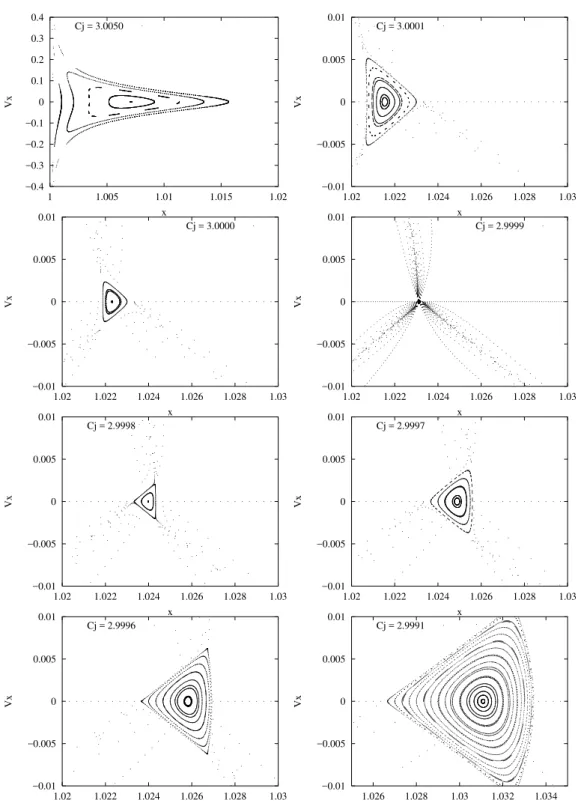
In order to explore the region of apparent stability shown in Fig. 1 we produced about thirty Poincar´e sur-faces of section. The range ofCjconsidered coincide with the range needed to cover the gray area given in Fig. 1 (2.9991 ≤ Cj ≤ 3.0050). A sample of the Poincar´e sur-faces of section generated are given in Fig. 2 . The center of the islands for each surface of section corresponds to one periodic orbit. They are members of a family of sim-ple retrograde periodic orbits called family “f” (Stromgren 1935).

0 0.2 0.4 0.6 0.8 1

0 0.5 1 1.5 2

Eccentricity

Semi−Major Axis (A.U) A

B

C

Fig. 1.Diagram indicating the initial conditions in terms ofa

versuse_{, taking}i₌ω_{= Ω = 0}◦_{andτ = 0, with capture times}

longer than 105

years (gray area). This plot was reproduced using the results from Vieira Neto & Winter (2001). The black lines correspond to contours of fixed values of Jacobi constant. The points A, B and C correspond to three particular periodic orbits.

2.2. Periodic orbits and stable regions

The center of the small island shown in the surface of section withCj= 2.9999 corresponds to the periodic orbit indicated by point B in Fig. 1. The largest islands curves give the size of the regular regions. The evolution of the size of the islands as the Jacobi constant decreases shows that the size of the regular regions decrease up to Cj = 2.9999 and then increase again (Fig. 2). The phenomenon which occurs atCj= 2.9999 has already been verified by other authors (H´enon 1970; Winter 2000) and it is due to the appearance of a 3:1 resonance (Arnold 1987). Note the change in the shape of the islands before and afterCj= 2.9999. That is equivalent to the change of the contours before and after point B (Fig. 1), from almost vertical lines to almost horizontal lines.

The size and location of the stable region associated to pericentric initial conditions can be determined by mea-suring the size and location of the largest islands of the surface of section. The horizontal width of the largest is-land for each surface of section (Fig. 2) can be converted into a pair of values of semi-major axis and eccentricity (Winter & Murray 1997a; Winter 2000). Proceeding with such computations, our results reveal that the stable re-gions from the surfaces of section corresponds exactly to the length of its Cj contour given in Fig. 1. Therefore, the apparently stable regions obtained computing capture times (Vieira Neto & Winter 2001) are in fact stable re-gions due to the quasi-periodic orbits associated to the periodic orbits of family “f”.

−0.4 −0.3 −0.2 −0.1 0 0.1 0.2 0.3 0.4

1 1.005 1.01 1.015 1.02

Vx

x Cj = 3.0050

−0.01 −0.005 0 0.005 0.01

1.02 1.022 1.024 1.026 1.028 1.03

Vx

x Cj = 3.0001

−0.01 −0.005 0 0.005 0.01

1.02 1.022 1.024 1.026 1.028 1.03

Vx

x

Cj = 3.0000

−0.01 −0.005 0 0.005 0.01

1.02 1.022 1.024 1.026 1.028 1.03

Vx

x

Cj = 2.9999

−0.01 −0.005 0 0.005 0.01

1.02 1.022 1.024 1.026 1.028 1.03

Vx

x Cj = 2.9998

−0.01 −0.005 0 0.005 0.01

1.02 1.022 1.024 1.026 1.028 1.03

Vx

x Cj = 2.9997

−0.01 −0.005 0 0.005 0.01

1.02 1.022 1.024 1.026 1.028 1.03

Vx

x Cj = 2.9996

−0.01 −0.005 0 0.005 0.01

1.026 1.028 1.03 1.032 1.034

Vx

x Cj = 2.9991

Fig. 2.Set of Poincar´e surfaces of section for different values of Jacobi constant,C_{j. The range of}C_{jconsidered in these plots}

coincide with the range needed to cover the gray area given in Fig. 1. The horizontal width of the largest island for each surface of section corresponds to the length of itsC_{j contour given in Fig. 1. The center of the small island shown in the surface of}

section withC_{j= 2}._{9999 corresponds to the periodic orbit indicated by point B in Fig. 1. Note the change in the shape of the}

islands before and afterCj= 2.9999. That is equivalent to the change of the contours before and after point B (Fig. 1), from almost vertical lines to almost horizontal lines. Also note the difference on the scales ofa_{for the first (top left corner) and the}

last (bottom right corner) plots.

than that of orbit A. However, the trajectories show an oval shape centered in the planet. The usual effects of such eccentricities can only be clearly seen from the trajectories draw in the non-rotating planetocentric system.

−0.05 −0.04 −0.03 −0.02 −0.01 0 0.01 0.02 0.03 0.04 0.05

0.95 0.97 0.99 1.01 1.03 1.05

y

x Baricentric Rotating

A B C

−0.05 −0.04 −0.03 −0.02 −0.01 0 0.01 0.02 0.03 0.04 0.05

−0.05 −0.03 −0.01 0.01 0.03 0.05

η

ξ

Non−Rotating Planetocentric

A B C

Fig. 3. Trajectories of the three simple periodic orbits A, B and C indicated in Fig. 1. From the trajectories draw in the

baricentric rotating system we can see that they originated from periodic orbits of the first kind (e_{≈0). The initial eccentricity}

of orbit C is higher than that of orbit B, which is higher than that of orbit A. However, the trajectories show an oval shape centered in the planet. The usual effects of such eccentricities can only be clearly seen from the trajectories in the non-rotating planetocentric system.

−0.02 −0.01 0 0.01 0.02

0.98 0.99 1 1.01 1.02

y

x a = 0.13873 e = 0.000

−0.02 −0.01 0 0.01 0.02

0.98 0.99 1 1.01 1.02

y

x a = 0.13868 e = 0.013

−0.02 −0.01 0 0.01 0.02

0.98 0.99 1 1.01 1.02

y

x a = 0.13933 e = 0.400

−0.02 −0.01 0 0.01 0.02

0.98 0.99 1 1.01 1.02

y

x a = 0.14672 e = 0.800

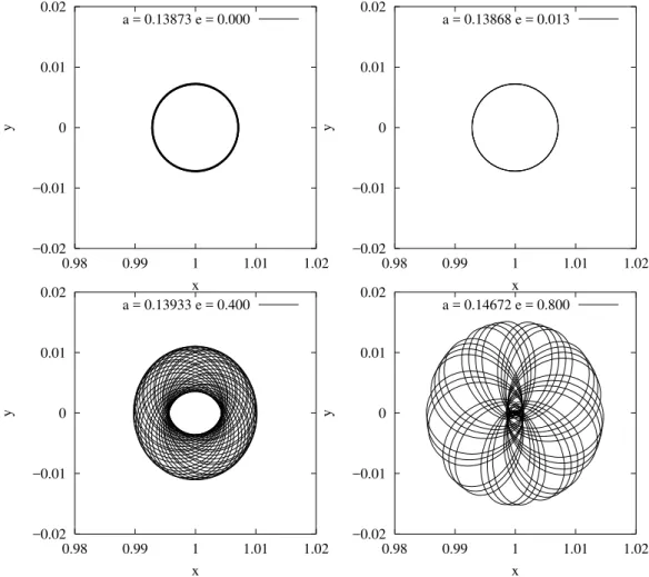
Fig. 4.Sample of stable orbits with C_{j = 3}._{005. All these trajectories have initial} a_≈0._{14 AU and their initial eccentricity is}

indicated in each plot. The trajectory corresponding to point A in Fig. 1 is the periodic orbit with initiale_{= 0}._{013. The other}

−0.06 −0.04 −0.02 0 0.02 0.04 0.06

0.94 0.96 0.98 1 1.02 1.04 1.06

y

x a = 1.400 e = 0.62904

−0.06 −0.04 −0.02 0 0.02 0.04 0.06

0.94 0.96 0.98 1 1.02 1.04 1.06

y

x a = 2.006 e = 0.70201

−0.06 −0.04 −0.02 0 0.02 0.04 0.06

0.94 0.96 0.98 1 1.02 1.04 1.06

y

x a = 2.400 e = 0.73946

−0.06 −0.04 −0.02 0 0.02 0.04 0.06

0.94 0.96 0.98 1 1.02 1.04 1.06

y

x a = 2.600 e = 0.75544

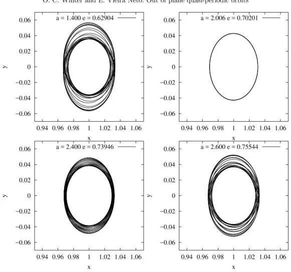
Fig. 5.Sample of stable orbits withCj= 2.9991. All these trajectories have initial eccentricity between 0.6 and 0.8, while their

initial semi-major axis is indicated in each plot. The trajectory corresponding to point C in Fig. 1 is the periodic orbit with

a_{= 2}._{006 AU. The other five trajectories shown are quasi-periodic orbits oscillating around the periodic orbit. Note that the}

amplitude of oscillation increases as the initial semi-major axis gets far from the value of the periodic orbit’s semi-major axis.

the cases withCj= 3.0050 andCj= 2.9991. A sample of stable orbits with Cj = 3.005 is presented in Fig. 4. All these trajectories have initiala≈0.1387 AU and their ini-tial eccentricity is indicated in each plot. The trajectory corresponding to point A in Fig. 1 is the periodic orbit with initial e = 0.013. The other five trajectories shown are quasi-periodic orbits oscillating around the periodic orbit. Note that the amplitude of oscillation increases as the initial eccentricity gets far from the value of the peri-odic orbit’s eccentricity.

A sample of stable orbits withCj= 2.9991 is presented in Fig. 5. All these trajectories have high initial eccentric-ity, between 0.6 and 0.8, while their initial semi-major axis are indicated in each plot. The trajectory corresponding to point C in Fig. 1 is the periodic orbit witha= 2.006 AU. The other five trajectories shown are quasi-periodic orbits oscillating around the periodic orbit. Note that the ampli-tude of oscillation increases as the initial semi-major axis gets far from the value of the periodic orbit’s semi-major axis.

The limiting case of this kind of periodic orbit can be seen as epicyclic orbits, as described in Chauvineau & Mignard (1990).

3. Stability of regions out of the plane

0 0.2 0.4 0.6 0.8 1

0 0.2 0.4 0.6 0.8 1

e a (A.U.) i=20o 0 0.2 0.4 0.6 0.8 1

0 0.2 0.4 0.6 0.8 1

e a (A.U.) i=30o 0 0.2 0.4 0.6 0.8 1

0 0.2 0.4 0.6 0.8 1

e a (A.U.) i=40o 0 0.2 0.4 0.6 0.8 1

0 0.2 0.4 0.6 0.8 1

e a (A.U.) i=50o 0 0.2 0.4 0.6 0.8 1

0 0.2 0.4 0.6 0.8 1

e a (A.U.) i=60o 0 0.2 0.4 0.6 0.8 1

0 0.2 0.4 0.6 0.8 1

e a (A.U.) i=70o 0 0.2 0.4 0.6 0.8 1

0 0.2 0.4 0.6 0.8 1

e a (A.U.) i=80o 0 0.2 0.4 0.6 0.8 1

0 0.2 0.4 0.6 0.8 1

e a (A.U.) i=110o 0 0.2 0.4 0.6 0.8 1

0 0.2 0.4 0.6 0.8 1

e a (A.U.) i=120o 0 0.2 0.4 0.6 0.8 1

0 0.2 0.4 0.6 0.8 1

e a (A.U.) i=130o 0 0.2 0.4 0.6 0.8 1

0 0.2 0.4 0.6 0.8 1

e a (A.U.) i=140o 0 0.2 0.4 0.6 0.8 1

0 0.2 0.4 0.6 0.8 1

e a (A.U.) i=150o 0 0.2 0.4 0.6 0.8 1

0 0.5 1 1.5 2

e a (A.U.) i=160o 0 0.2 0.4 0.6 0.8 1

0 0.5 1 1.5 2

e a (A.U.) i=170o 0 0.2 0.4 0.6 0.8 1

0 0.5 1 1.5 2

e

a (A.U.) i=180o

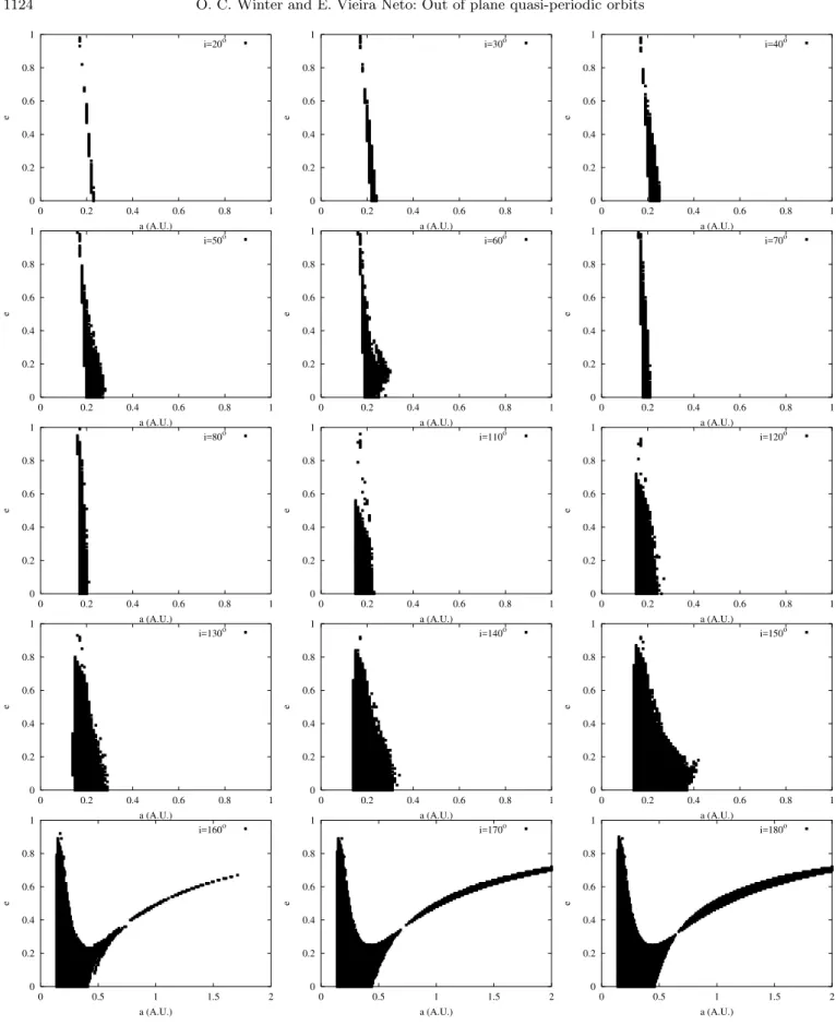
Fig. 6.Set of diagrams showing the initial conditions in terms ofa_versuse_{, taking}ω_{= Ω = 0}◦_{andτ= 0, with capture times}

longer than 105

−0.01 −0.005 0 0.005 0.01

0.99 0.995 1 1.005 1.01

y

x i=180o

−0.01 −0.005 0 0.005 0.01

0.99 0.995 1 1.005 1.01

z

x i=180o

−0.01 −0.005 0 0.005 0.01

0.99 0.995 1 1.005 1.01

y

x i=140o

−0.01 −0.005 0 0.005 0.01

0.99 0.995 1 1.005 1.01

z

x i=140o

−0.01 −0.005 0 0.005 0.01

0.99 0.995 1 1.005 1.01

y

x i=120o

−0.01 −0.005 0 0.005 0.01

0.99 0.995 1 1.005 1.01

z

x i=120o

Fig. 7.Sample of stable orbits with the same initial eccentricity,e_{= 0}._{013. The initial inclination of each trajectory is indicated}

on the plot. The trajectories are shown projected in theXY _{plane (left column) and in the}XZ _{plane (right column). The}

periodic orbit A is shown in the first pair of plots. The other two pairs of plots present 3-D quasi-periodic orbits around the planar periodic one. Note that the amplitude of oscillation increases as the initial inclination decreases.

From Fig. 6 we can see that the largest region for prograde orbits occurs at i = 60◦_{. While in the case} of retrograde orbits the largest region occurs at i = 180 deg. We can also note that there is no prograde or-bit with a ≥ 0.32 AU, while there are retrograde orbits with a ≥ 2 AU. Hamilton & Burns (1991) studied the forces components acting on the problem of initially cir-cular trajectories. They concluded that in the planar case

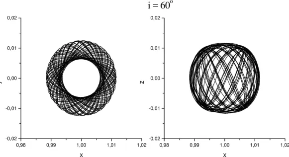
0,98 0,99 1,00 1,01 1,02 -0,02

-0,01 0,00 0,01 0,02

z

x

0,98 0,99 1,00 1,01 1,02

-0,02 -0,01 0,00 0,01 0,02

y

x

i = 60

Fig. 8. A regular orbit with initial inclination of 60◦_{. The trajectory is shown projected in theXY plane (top view) and in}

the XZ_{plane (edge on). Note that the behavior of this trajectory is very much similar to the quasi-periodic orbit with initial}

inclination of 120◦_{shown in Fig. 7, but with a larger amplitude of oscillation.}

retrograde prisoner trajectories was found to be the exis-tence of the family of periodic orbits “f” and the quasi-periodic orbits oscillating around them. Therefore, one could expect that there would be periodic orbits out of the plane in order to explain the existence of the inclined prisoner trajectories shown in Fig. 6. Therefore, we per-formed a search for such periodic orbits without success.

3.1. Tridimensional retrograde orbits

Exploring the orbital evolution of inclined retrograde pris-oner trajectories we identified a pattern related to the pla-nar periodic orbits of family “f”. A sample of such orbits with the same initial eccentricity,e= 0.013, but different initial inclinations is given in Fig. 7. The initial inclination of each trajectory is indicated on the plot. The trajecto-ries are shown projected in the XY plane (left column) and in the XZ plane (right column). The periodic orbit A is shown in the first pair of plots. The other three pairs of plots shown suggest that they are tridimensional quasi-periodic orbits oscillating around the planar quasi-periodic one. Note that the amplitude of oscillation increases as the ini-tial inclination decreases. However, that is not the case for all the retrograde prisoner trajectories given in Fig. 6. The trajectories on the borders of the regions (black ar-eas) do not show quasi-periodic orbit’s behavior despite of the fact that these trajectories did not escape for an inte-gration period of 105 _{years. Such trajectories will escape} later. The trajectories are similar to the case shown in Figs. 12 and 13 of Hamilton & Burns (1991). That might be explained because of the problem’s fractal-like nature (Murison 1989). They show a sort of sticking phenomenon (Winter & Murray 1995).

3.2. Tridimensional prograde orbits

In the case of inclined prograde prisoner trajectories, the results are not much different from the inclined retrograde case. In Fig. 8 we present a regular orbit with initial in-clination of 60◦_{. The trajectory is shown projected in the} XY plane and in theXZplane. Note that the behavior of this trajectory is very much similar to the quasi-periodic orbit with initial inclination of 120◦_{shown in Fig. 7, but} with a larger amplitude of oscillation. Therefore, that would mean that the inclined prograde prisoner trajec-tories would be tridimensional quasi-periodic orbits os-cillating around the planar periodic orbit of family “f”. Similarly to the inclined retrograde prisoner trajectories region, the trajectories on the borders of the regions (gray areas) do not show quasi-periodic orbit’s behavior for the same reason.

Acknowledgements. We would like to thanks T. Stuchi and A. A. Corrˆea for some fruitful discussions on periodic orbits out of the plane. This work was partially funded by Fapesp (Proc. 98/15025-7) and Fundunesp (Proc. 458/2000-DFP). These supports are gratefully acknowledged. We also would like to thanks Dr. N. Gorkavyi for the advice and the com-ments on this paper.

References

Arnold, V. I. 1987, M´etodos Matem´aticos da Mecˆanica Cl´assica (Editora Mir, Moscow)

Benest, D. 1971, A&A, 13, 157 Benest, D. 1974, A&A, 32, 39 Benest, D. 1975, A&A, 45, 353 Benest, D. 1976, A&A, 53, 231 Benest, D. 1977, A&A, 54, 568

Chauvineau, B., & Mignard, F. 1990, Icarus, 83, 360 Gorkavyi, N. 1993, Astron. Lett., 19(6), 448

Hamilton, D. P., & Burns, J. A. 1991, Icarus, 92, 118 Hamilton, D. P., & Krivov, A. V. 1997, Icarus, 128, 241 H´enon, M. 1965a, Ann. Astr., 28, 499

H´enon, M. 1965b, Ann. Astr., 28, 992

H´enon, M. 1966a, Bull. astr., Paris, 1, fasc. 1, 57 H´enon, M. 1966b, Bull. astr., Paris, 1, fasc. 2, 49 H´enon, M. 1969, A&A, 1, 223

H´enon, M. 1970, A&A, 9, 24

Huang, T. Y., & Innanen, K. A. 1983, AJ, 88, 10

Jefferys, W. H. 1971, An Atlas of Surfaces of Section for the Restricted Three Bodies University of Texas, Austin Murison, M. A. 1989, AJ, 98, 2346

Stromgren, E. 1935, Bull. Astr., Paris, 9, 87

Vieira Neto, E., & Winter, O. C. 2001, AJ, 122, 1, 440 Winter, O. C., & Murray, C. D. 1994a, Atlas of the planar,

circular, restricted three-body problem. I. Internal Orbits, QMW Maths Notes, No. 16 (Queen Mary and Westfield College, London, UK)

Winter, O. C., & Murray, C. D. 1994b, Atlas of the planar, cir-cular, restricted three-body problem. II. External Orbits, QMW Maths Notes, No. 17 (Queen Mary and Westfield College, London, UK)

Winter, O. C., & Murray, C. D. 1995, In From Newton to Chaos, NATO ASI Series B: Phys., 336, 193