Time analysis for temporary gravitational capture: Satellites of Uranus

(1)

THEASTRONOMICALJOURNAL, 122 : 440È448, 2001 July

TIME ANALYSIS FOR TEMPORARY GRAVITATIONAL CAPTURE : SATELLITES OF URANUS E. VIEIRANETO1ANDO. C. WINTER

Grupo deDinaümicaOrbital e Planetologia, Departamento deMatematica,Universidade Estadual Paulista, C.P. 205, 12500-000Guaratingueta,SP, Brazil ;ernesto=feg.unesp.br, ocwinter=feg.unesp.br

Received 2000 May 23 ; accepted 2001 March 28

ABSTRACT

We study the problem of gravitational capture in the framework of the Sun-Uranus-particle system. Part of the space of initial conditions is systematically explored, and the duration of temporary gravita-tional capture is measured. The location and size of di†erent capture-time regions are given in terms of diagrams of initial semimajor axis versus eccentricity. The other initial orbital elementsÈinclination (i), longitude of the node ()), argument of pericenter (u), and time of pericenter passage (q)Èare Ðrst taken to be zero. Then we investigate the cases with u\90¡, 180¡, and 270¡. We also present a sample of results for )\_{90¡, considering the cases} _i\_{60¡, 120¡, 150¡, and 180¡. Special attention is given to the} inÑuence of the initial orbital inclination, taking orbits initially in opposition at pericenter. In this case, the initial inclination is varied from 0¡ to 180¡ in steps of 10¡. The success of the Ðnal stage of the capture problem, which involves the transformation of temporary captures into permanent ones, is highly dependent on the initial conditions associated with the longest capture times. The largest regions of the initial-conditions space with the longest capture times occur at inclinations of 60¡È70¡ and 160¡. The regions of possible stability as a function of initial inclination are also delimited. These regions include not only a known set of retrograde orbits, but also a new sort of prograde orbit with inclinations greater than zero.

Key words :celestial mechanics È minor planets, asteroids È planets and satellites : general È planets and satellites : individual (Uranus)

1

.

INTRODUCTION

The diversity and quantity of moons in the outer solar system is remarkable. Most of these moons, called regular satellites, were probably formed in a protosatellite disk around their planets. These satellites have quasi-circular orbits close to the planetÏs equatorial plane and also are not too far from it (less than 100 planetary radii). How-ever, there are some moons with orbits very di†erent from these, with high eccentricity, high inclination (some are retrograde), and, for most of them, semimajor axes of more than a hundred planetary radii. All the giant planets have irregular satellites, but only in 1997 were the Ðrst irregular moons around Uranus discovered (Gladman et al. 1998). Such irregular planetary satellites may possibly be captured asteroids, as noted by Kuiper (1961). Nevertheless, a purely gravitational mechanism cannot stabilize an orbit around a planet, as proved by Hopf (1930). Some kind of dissipative force is necessary to accomplish the capture. Pollack, Burns, & Tauber (1979) have given some examples of these forces. In general, gas drag is the most efficient, as a result of its ability to reduce the semimajor axis, eccentricity, and incli-nation of the orbit (Hunten 1979).

In general, gravitational capture is studied in the frame-work of the restricted three-body problem, with numerical simulations. The complexity of this problem can be seen in Cordeiro, Viera Martins, & Leonel (1999). However, a precise deÐnition of gravitational capture has not been well established. For example, Heppenheimer (1975) deÐned capture as the passage of the particle by the colinear Lagrangian point L1. Huang & Innanen (1983) used initial conditions satisfying the mirror theorem, and the orbit was considered to be in the capture region (as deÐned by Henon

ÈÈÈÈÈÈÈÈÈÈÈÈÈÈÈ

1Postdoctoral program.

1970) if the particles did not escape from this region in a period of time between 10 and 1000 years.

As pointed out by Brunini (1996), dissipative di†usion is, in general, a slow process, so captures with long times increase the probability of permanent capture. Therefore, the study of the duration of gravitational capture is relevant because it provides important information about the kind of dissipative process that can turn a temporary capture into a permanent one.

In the present work, we study the capture time, i.e., the length of temporary gravitational capture. We have chosen the Sun-Uranus system to perform this research. The moons discovered by Gladman et al. (1998) are not in the capture region, they have Jacobi constants greater than the value for the L1 Lagrangian point for the Sun-Uranus system, and therefore they are in a stable region. However, they are the main motivation for this research.

Heppenheimer & Porco (1977), using a di†erent approach, also studied the lifetimes of satellites in the prox-imity of the central body. They created an analytical method by which to estimate the capture time. However, their theory only provides order-of-magnitude estimates, thought rather conservative.

The deÐnition used here for capture is taken from Yama-kawa (1992). In his concept, a parameter deÐned as the two-body energy due to the planet-particle system is moni-tored. A trajectory that begins with an elliptical orbit around the planet has a negative value of this parameter. When its sign turns from negative to positive, the trajectory changes from an ellipse to a hyperbola, i.e., the particle escapes from the gravitational domain of the planet. This escape trajectory is also a captured one if the time propaga-tion is inverted.

We explore the capture time for a wide range of initial conditions using a purely gravitational mechanism. In the next section, we present the approach adopted in the

(2)

TEMPORARY GRAVITATIONAL CAPTURE 441

present work. Section 3 contains the results in terms of diagrams of semimajor axis versus eccentricity. The capture times given in these diagrams are statistically analyzed. The e†ect of the noncircularity of UranusÏs orbit and the e†ects of perturbations due to Jupiter, Saturn, and both together are studied. Some Ðnal considerations are given in the last section.

2

.

THE GRAVITATIONAL CAPTURE APPROACH

We have considered the three-dimensional circular restricted three-body problem, for the Sun, Uranus, and a particle, as our standard dynamical system. The trajectories are integrated from initial conditions in the vicinity of the planet until the particle escapes. A negative time step is used, so the escape trajectory is a capture one when the time is stepped forward. The initial conditions are the orbital elements of the particle relative to Uranus (planetocentric orbital elements).

This circular restricted three-body system is not integra-ble, and its total energy and angular momentum are not conserved. Nevertheless, it has an integral of the motion, the Jacobi constant,C_J. The value of this constant is used to determine whether a trajectory can escape from the planet or not.

The procedure adopted to characterize a gravitational capture is the same as that presented by Yamakawa (1992). The idea is based on monitoring of the two-body orbital energy, deÐned as

E\v2

2 [

k

r , (1)

wherevis the particleÏs velocity in the Ðxed system,ris its orbital radial distance, andkis the mass parameter.

The two-body (Uranus-particle) energy is not constant, because of the perturbation of the third body (the Sun). The value ofEalong the trajectory gives a clue to which body (the Sun or Uranus) exerts the dominant gravitational inÑu-ence on the particleÏs trajectory. Vieira Neto (1999) made extensive experiments withE, showing that this parameter efficiently characterizes temporary gravitational capture. The changing of the energyÏs sign indicates that the oscu-lating orbit has switched from closed to open (escape) or from an open orbit to a closed one (capture).

3

.

CAPTURE TIME

As stated above, a di†usion process is necessary to turn a temporary gravitational capture into a permanent one. This process is slow and needs a relatively long time to be e†ec-tive. Therefore, it is relevant to locate gravitational capture trajectories that remain around the planet for a long time. Such trajectories are potential candidates for the initial con-ditions of the known irregular satellites.

In this section, we present a systematic and detailed exploration relative to the problem of timing in temporary capture. With an extensive numerical study, it is possible to classify regions of the space of initial conditions according to their capture times. A grid of initial orbital conditions is deÐned, and we generate gray-scale images representing the distribution of the capture times in the space of semimajor axis versus eccentricity.

The following Ðgures show how the capture time varies depending on the initial conditions. Each image comprises a grid of semimajor axis and eccentricity, taking the initial

values of the other orbital elements as Ðxed. The orbital elements are relative to Uranus. The grid of semimajor-axis initial values starts at 0.01 AU and goes to 2 AU, in steps of 0.01 AU. The eccentricity initial value runs from 0 to 0.99, in steps of 0.01. Thus, each point in the image corresponds to one trajectory. Each trajectory is integrated with a negative time step from zero to[50,000 yr.

As a result of the conÐguration of the initial orbital ele-ments, the initial two-body energy, relative to Uranus, has a negative value (closed orbit around the planet). With the perturbation from the third body (the Sun), the energy changes value. When the value of the orbital energy becomes positive (open orbit), it is considered an escape and the integration is interrupted. The time elapsed from the initial conditions to the escape condition is stored. We refer to this time as the capture time, atlhough the actual length of time for a temporary capture is higher than this value. For initial conditions satisfying the mirror theorem (Roy & Ovenden 1955), the values for the capture time are in fact twice the values indicated in this paper. This is the case for most of the trajectories considered here.

The numerical integrations were also stopped if the par-ticle had a collision with the planet or if the integration time surpassed[_{50,000 yr. If the particle does not escape within} a period of 50,000 yr, its trajectory is referred to as a ““ prisoner ÏÏ orbit.

In the Ðgures, the solid lines indicate the zero-velocity curve withC_J\C_J,L1.Therefore, these lines deÐne limits for the sets of initial conditions that can generate temporary capture trajectories for the restricted three-body problem. White regions inside these lines represent initial conditions for prisoner trajectories. The planetary collision trajec-tories, those that collide with Uranus, are indicated by plus signs.

3.1. Planar Case

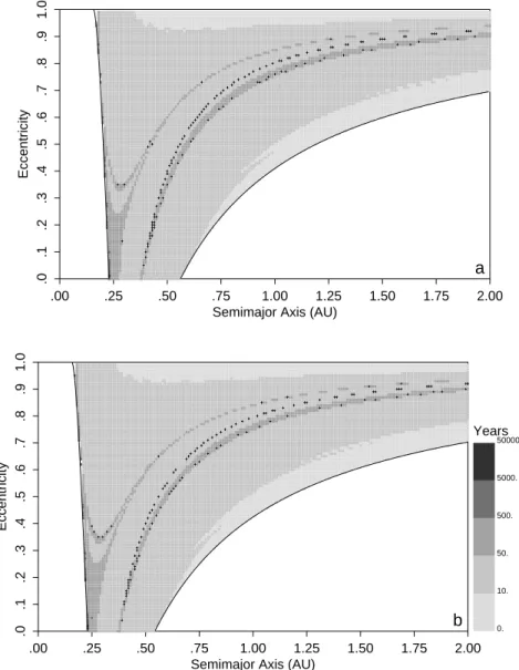
The prograde planar case is studied Ðrst. We examine the dependence of the capture times for di†erent values of the longitude of pericenter, u. Figure 1 shows two outcomes. The di†erences are in the initial value of the longitude of pericenter :u\0¡ in Figure 1a, andu\180¡ in Figure 1b. The other two orbital elements are)\0¡ andq\0.

Because of the geometry of the orbits in Figure 1a, the initial positions of the particles correspond to opposition to the Sun, and in Figure 1bthey are in inferior conjunction. Nevertheless, the structures are very similar in terms of the capture times. It can be seen that the shortest times are dominant. In general, the capture times are shorter than 500 yr, which is less than about four Keplerian orbital periods in the case of semimajor axes greater than 1 AU.

Capture times between 50 and 500 yr, which exhibit a bow-shaped region in the middle of both panels, are sur-rounded by collisions. A speciÐc conÐguration of semimajor axis and eccentricity gives rise to an almost well deÐned curve for the collisions. There is high instability in the neighborhood of this curve, and the behavior of the trajec-tory is sensitive to small changes in the initial conditions. There are three possibilities : (1) collisions, (2) rapid escape (10È50 yr), and (3) trajectories that take a longer time to escape (50È500 yr). There are also a few trajectories with capture times between 5000 and 50,000 yr and even higher than 50,000 yr (the white regions in the upper left corner).

(3)

.00 .25 .50 .75 1.00 1.25 1.50 1.75 2.00 Semimajor Axis (AU)

.0

.1

.2

.3

.4

.5

.6

.7

.8

.9

1.0

Eccentricity

a

.0

.1

.2

.3

.4

.5

.6

.7

.8

.9

1.0

Eccentricity

0. 10. 50. 500. 5000. 50000. Years

b

442 VIEIRA NETO & WINTER Vol. 122

FIG. 1.ÈCapture times in the initial-conditions space of semimajor axis vs. eccentricity. Time, in years, is represented by the gray scale. The range of initial

conditions considered is delimited by the zero-velocity curves associated with L1 (solid lines). The particles are initially at pericenter with i\0¡ and (a)u\0¡ or (b)u\180¡. The other orbital elements are)\0¡ andq\0. The white regions inside the range of initial conditions considered correspond to trajectories that exceed 50,000 yr without escape (““ prisoner ÏÏ trajectories). Plus signs correspond to collision trajectories.

other orbital elements are the same as in Figure 1. This change generates di†erent structures for the capture times. These sets of initial conditions do not satisfy the mirror theorem ; nevertheless, computations of the numerical inte-grations forward in time for these initial conditions conÐrm that the capture times are roughly double the values pre-sented in Figures 2aand 2b.

The structure seen in Figure 2a is very much similar to that in Figure 2b. They mainly present short capture times, which seem to be a characteristic of planar, prograde orbits, independent of the value ofu. The main contrast between Figures 1 and 2 is the collision trajectories that occur for the cases in whichu\90¡ oru\270¡. One can also note that the prisoner orbits (white region) are at lower values of eccentricity in those cases.

3.2. Inclined Case

In this subsection, we explore the inÑuence of orbital inclination on the capture time. Figure 3 shows the results for a range of inclinations from 10¡ to 180¡, in steps of 10¡, and taking)\0¡,u\0¡, andq\0.

Short capture times (¹500 yr) dominate the space of initial conditions. However, one of the most important fea-tures of Figure 3 is the evolution in the quantity of prisoner orbits as the inclination increases. The number of these tra-jectories increases and occupies larger regions of the space. Initially, at i\0¡ (Fig. 1a), there are almost no prisoner orbits. As the inclination increases, the number of prisoner orbits starts to grow, occupying a region of low semimajor-axis values, but for almost all values of eccentricity. When the value of the inclination reaches 160¡ (Fig. 3p), a narrow strip of prisoner orbits appears. It is interesting to note that for i\150¡ (just 10¡ apart), this same region in the a-e diagram is full of short capture times (Fig. 3o). The narrow strip becomes wider as the initial inclination increases. It reaches its apex fori\180¡ (Fig. 3r), the planar retrograde orbits.

(4)

.0

.1

.2

.3

.4

.5

.6

.7

.8

.9

1.0

Eccentricity

a

.0

.1

.2

.3

.4

.5

.6

.7

.8

.9

1.0

Eccentricity

0. 10. 50. 500. 5000. 50000. Years

b

No. 1, 2001 TEMPORARY GRAVITATIONAL CAPTURE 443

FIG. 2.ÈSame as Fig. 1, but for particles initially at pericenter withi\0¡ and (a)u\90¡ or (b)u\270¡

prisoner trajectories. This process occurs gradually, as the inclination rises from 110¡ to 180¡.

For the i\180¡ case (retrograde orbits), a sample of initial conditions inside the narrow strip (prisoner trajectories) was numerically integrated for 10 Myr, and the trajectories did not escape. This region is associated with the stability of retrograde orbits detected byHenon(1970) and also studied by several other authors, for the planar case (i\_{180¡). The stability of retrograde orbits for the} spatial case (160¡¹i\180¡) and the prograde case (i^60¡) is studied in Winter & Vieira Neto (2001).

Part of the structure seen in Figure 3r(i\180¡) can be compared to the results of Huang & Innanen (1983). In their work, the stability regions were determined for planar retrograde orbits in the Sun-Jupiter-particle system. The location of the prisoner trajectories in our Figure 3ris in good agreement with Figure 2 of their work.

Huang & Innanen (1983) also suggested that the initial conditions that cause long capture times should be near the stability boundaries in the phase space around the planet. Our results conÐrm that the long capture times are near the borders of the prisoner trajectories. However, it can be seen that the distribution of capture times along such boundaries

is not uniform. For instance, in Figure 3rit is possible to see a high concentration of long capture times (500È5000 yr) only around (a,e)\(0.58, 0.33).

Figure 4ashows the percentage of trajectories that collide with the planet and the percentage of trajectories that remain imprisoned within a period of 50,000 yr for each inclination. These data were obtained from Figure 1a and Figure 3. For prograde orbits, 0¡¹i\90¡, there are few collisions. At each inclination in this range, fewer than 1% of the trajectories collide with the planet. At 90¡ inclination, more than 2% of the trajectories result in collisions. At i\100¡, the number of collisions increases a bit and starts to decrease slowly. The majority of the collisions occur for small values of the semimajor axis,a\0.3 AU.

(5)

.0

.1

.2

.3

.4

.5

.6

.7

.8

.9

1.0

Eccentricity

a

.0

.1

.2

.3

.4

.5

.6

.7

.8

.9

1.0

Eccentricity

0. 10. 50. 500. 5000. 50000. Years

b

.0

.1

.2

.3

.4

.5

.6

.7

.8

.9

1.0

Eccentricity

c

.0

.1

.2

.3

.4

.5

.6

.7

.8

.9

1.0

Eccentricity

d

.0

.1

.2

.3

.4

.5

.6

.7

.8

.9

1.0

Eccentricity

e

.0

.1

.2

.3

.4

.5

.6

.7

.8

.9

1.0

Eccentricity

0. 10. 50. 500. 5000. 50000. Years

f

444 VIEIRA NETO & WINTER

FIG. 3.ÈSame as Fig. 1, but for particles initially at pericenter withu\0¡ and orbital inclination varying from 10¡ to 180¡ with*i\10¡ in (a)È(r),

respectively.

Since the prisoner orbits might be regular (periodic and quasi-periodic orbits), they are not candidate temporary capture orbits unless the dynamical system is altered in order to include other perturbations. Therefore, the orbits with high capture times, 500È5000 and 5000È50,000 yr, become the most relevant to this study. From Figure 3, it can be seen that such orbits are located on the borders of the region dominated by the prisoner trajectories. Figure 4b shows the percentage of these trajectories as a function of initial inclination. The number of trajectories with high capture times is relatively small. For trajectories with capture times between 5000 and 50,000 yr, there are peaks at i\60¡ and at i\160¡. For trajectories with capture times in the interval 500È5000 yr, the peaks occur ati\_70¡ and at i\160¡. From Figure 4a it can be seen that the

maxima in the distribution of prisoner trajectories are close to the maxima of these groups of capture times. This means that where there exist more stable orbits (the prisoner orbits), there are a larger number of trajectories with long capture times. This relation enhances the probability of capture in such locations. Another important fact is that for planar retrograde orbits (i\180¡), there are few trajectories with long capture times. The capture probability in this case is lower than for the case described above (i\60¡ and i\_160¡).

(6)

.0

.1

.2

.3

.4

.5

.6

.7

.8

.9

1.0

Eccentricity

g

.0

.1

.2

.3

.4

.5

.6

.7

.8

.9

1.0

Eccentricity

h

.0

.1

.2

.3

.4

.5

.6

.7

.8

.9

1.0

Eccentricity

i

.0

.1

.2

.3

.4

.5

.6

.7

.8

.9

1.0

Eccentricity

0. 10. 50. 500. 5000. 50000. Years

j

.0

.1

.2

.3

.4

.5

.6

.7

.8

.9

1.0

Eccentricity

k

.0

.1

.2

.3

.4

.5

.6

.7

.8

.9

1.0

Eccentricity

l

.0

.1

.2

.3

.4

.5

.6

.7

.8

.9

1.0

Eccentricity

m

.0

.1

.2

.3

.4

.5

.6

.7

.8

.9

1.0

Eccentricity

0. 10. 50. 500. 5000. 50000. Years

n

(7)

.0

.1

.2

.3

.4

.5

.6

.7

.8

.9

1.0

Eccentricity

o

.0

.1

.2

.3

.4

.5

.6

.7

.8

.9

1.0

Eccentricity

p

.0

.1

.2

.3

.4

.5

.6

.7

.8

.9

1.0

Eccentricity

q

.0

.1

.2

.3

.4

.5

.6

.7

.8

.9

1.0

Eccentricity

0. 10. 50. 500. 5000. 50000. Years

r

0 0.2 0.4 0.6 0.8 1 1.2 1.4

0 20 40 60 80 100 120 140 160 180

Trajectories percentage

Inclination (degrees) b 500−5000 years

5000−50000 years 0

2 4 6 8 10 12 14

0 20 40 60 80 100 120 140 160 180

Inclination (degrees) a Colision

Prisioner

0 10 20 30 40 50 60 70 80

0 to 10 10 to 50 50 to 500 500 to 5000 5000 to 50000

Years

446 VIEIRA NETO & WINTER Vol. 122

FIG. 3.ÈContinued

FIG. 4.ÈPercentage distribution of trajectories as a function of

inclina-tion. (a) Prisoner and collision trajectories, i.e., those that exceed 50,000 yr without escape and those that collide with Uranus. (b) A group of trajec-tories with long capture times, 500È5000 and 5000È50,000 yr. For each set of initial conditions, the inclination varies from 0¡ to 180¡ withu\0¡.

yielding the percentage of trajectories in the time interval for each inclination. The points are the mean and the error bars are the standard deviation for each time interval, taking into account the inclinations from 0¡ to 180¡. Con-sidering that the interval from 0 to 10 yr is a subinterval of that from 0 to 50 yr, it is possible to Ðt an exponential curve to the distribution of trajectories. The results show that 86.51% of the trajectories have capture times shorter than 50 yr, 12.48% are in the capture-time interval from 50 to 500 yr, and just about 1% are in the two subsequent inter-vals (see Fig. 4b).

Computation of the capture times for di†erent values of the longitude of pericenter and the longitude of the node reveals a simpler structure to the semimajor-axis versus

FIG. 5.ÈDistribution of temporary capture trajectories as a function of

(8)

.0

.1

.2

.3

.4

.5

.6

.7

.8

.9

1.0

Eccentricity

a

.0

.1

.2

.3

.4

.5

.6

.7

.8

.9

1.0

Eccentricity

b

.0

.1

.2

.3

.4

.5

.6

.7

.8

.9

1.0

Eccentricity

c

.0

.1

.2

.3

.4

.5

.6

.7

.8

.9

1.0

Eccentricity

0. 10. 50. 500. 5000. 50000. Years

d

No. 1, 2001 TEMPORARY GRAVITATIONAL CAPTURE 447

eccentricity space. They do not present prisoner trajectories with initial conditions far from the planet. In those cases the furthest prisoner trajectories found havea(1]_e₎_\_{0.6 AU.}

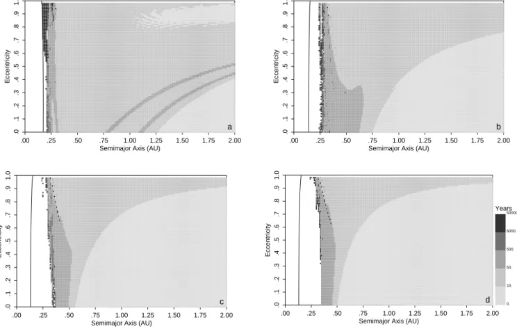
Figure 6 shows the structure of the capture times for initial values of )\90¡, u\0¡, and q\0. The inclina-tions arei\_{60¡ (Fig. 6}_a_), _i\_{120¡ (Fig. 6}_b_),_i\_{150¡ (Fig.} 6c), andi\180¡ (Fig. 6d). For the planar case (i\0¡ and i\_{180¡), the ascending node (}₎_{) is not deÐned. Thus, for} i\0¡ the results presented in Figure 2a for )\0¡ and u\_{90¡ are the same for}₎\_{90¡ and}_u\_0¡.

In our computations we also found that at i\90¡ the prisoner trajectories change to collision trajectories in the same way as shown in Figure 3. The initial conditions for these Ðgures do not obey the mirror theorem, but as stated above, the total times for temporary gravitational capture are almost twice those given by the scale shown in Figure 6.

The distribution of the capture times for)\_{90¡ is very} di†erent from and less interesting than the anterior case, )\0¡. Nevertheless, the locations of high capture times are also in the proximity of the border of the prisoner region.

3.3. Perturbations

In order to estimate the inÑuence of the eccentricity and inclination of UranusÏs orbit and the gravitational pertur-bations due to Jupiter and Saturn in our results, we per-formed some sample numerical simulations. The tests were made, and compared, with the case of Figure 3r: i\_180¡,

)\0¡,u\0¡, andq\0.

The complexity of the system was increased gradually. First, the trajectories of the particles were simulated with

the eccentricity of Uranus. The region of prisoner trajec-tories changes very slightly, mainly for low values of the eccentricity of the particle and for low semimajor-axis values.

The inclination of Uranus has much less of an e†ect than does the eccentricity. The trajectories were also simulated with the presence of Jupiter, Saturn, and both together. Saturn presented a stronger e†ect than Jupiter, but neither of them signiÐcantly modiÐed the structure of the capture-time diagram. The presence of both planets has an e†ect very similar to that of Saturn alone.

4

.

FINAL CONSIDERATIONS

The study of capture times presented here a†ords material for the second stage of the gravitational capture problem : the change of a temporary gravitational capture into a permanent one. The results presented show the detailed structure of the main part of the initial-conditions space in terms of the capture time. In particular, we have localized the longest capture times. It is interesting to explore the behavior of particles near these trajectories when a dissipative force is applied. In general, these forces are small perturbations compared with the gravitational forces involved. Therefore, it is necessary for a satellite to orbit for a relatively long time to su†er their e†ects and be converted into a permanent satellite.

Another relevant result presented in this work is the loca-tion of the possibly stable region observed for retrograde orbits at a large distance from the planet. Benest (1971) and Huang & Innanen (1983), among others, studied similar

FIG. 6.ÈSame as Fig. 1, but for particles initially at pericenter with (a)i\60¡, (b)i\120¡, (c)i\150¡, and (d)i\180¡. The other orbital elements are

(9)

448 VIEIRA NETO & WINTER

regions for Jupiter. However, they presented results only for the planar case. In the present work, it was possible to identify these regions not just for retrograde orbits but also for a whole range of di†erent initial inclinations. The results show that these regions also exist for prograde orbits.

The e†ects due to UranusÏs eccentricity and inclination and the perturbations of Jupiter and Saturn do not signiÐ-cantly a†ect the structure of capture times given by the

restricted three-body retrograde case. Many details of the available phase space still remain unexplored and will require additional studies.

This work was partially funded by the Brazilian agencies FAPESP under grant 98/15025-7 and Fundunesp under grant 458/2000-DFP. This support is gratefully acknowl-edged.

REFERENCES Benest, D. 1971, A&A, 13, 157

Brunini, A. 1996, Celest. Mech. Dyn. Astron., 64, 79

Cordeiro, R. R., Viera Martins, R., & Leonel, E. D. 1999, AJ, 117, 1634 Gladman, B. J., Nicholson, P. D., Burns, J. A., Kavelaars, J. J., Marsden,

B. G., Williams, G. V., & O†utt, W. B. 1998, Nature, 392, 897 M. 1970, A&A, 9, 24

Henon,

Heppenheimer, T. A. 1975, Icarus, 24, 172

Heppenheimer, T. A., & Porco, C. 1977, Icarus, 30, 385 Hopf, E. 1930, Math. Ann., 103, 710

Huang, T.-Y., & Innanen, K. A. 1983, AJ, 88, 1537

Hunten, D. M. 1979, Icarus, 37, 113

Kuiper, G. P. 1961, in The Solar System, Vol. 3, Planets and Satellites, ed. G. P. Kuiper & B. M. Middlehurst (Chicago : Univ. Chicago Press), 575 Pollack, J. B., Burns, J. A., & Tauber, M. E. 1979, Icarus, 37, 587 Roy, A. E., & Ovenden, M. W. 1955, MNRAS, 115, 296

Vieira Neto, E. 1999, Ph.D. thesis, Inst. Nac. Pesquisas Espaciais (INPE-7033-TDI/663)