Atmospheric transport and chemistry of trace gases in LMDz5B: evaluation and implications for inverse modelling

(1)

GMDD

7, 4993–5048, 2014

Atmospheric transport in LMDZ

R. Locatelli et al.

Title Page

Abstract Introduction

Conclusions References

Tables Figures

◭ ◮

Back Close

Full Screen / Esc

Printer-friendly Version Interactive Discussion

Discussion

P

a

per

|

Discus

sion

P

a

per

|

Discussion

P

a

per

|

Discussion

P

a

per

Geosci. Model Dev. Discuss., 7, 4993–5048, 2014 www.geosci-model-dev-discuss.net/7/4993/2014/ doi:10.5194/gmdd-7-4993-2014

This discussion paper is/has been under review for the journal Geoscientific Model Development (GMD). Please refer to the corresponding final paper in GMD if available.

Atmospheric transport and chemistry of

trace gases in LMDz5B: evaluation and

implications for inverse modelling

R. Locatelli1, P. Bousquet1, F. Hourdin2, M. Saunois1, A. Cozic1, F. Couvreux3,

J.-Y. Grandpeix2, M.-P. Lefebvre2,3, C. Rio2, P. Bergamaschi4, S. D. Chambers5,

U. Karstens6, V. Kazan1, S. van der Laan*, H. A. J. Meijer7, J. Moncrieff8,

M. Ramonet1, H. A. Scheeren4,7, C. Schlosser9, M. Schmidt1,**, A. Vermeulen10,

and A. G. Williams5

1

Laboratoire des Sciences du Climat et de l’Environnement (LSCE), Gif-sur-Yvette, France

2

Laboratoire de Meteorologie dynamique (LMD) – Jussieu, Paris, France

3

Centre National de Recherches Météorologiques (CNRM-Game), Météo-France, Toulouse, France

4

Institute for Environmental and Sustainability, Joint Research Centre, European Commission, Ispra, Italy

5

Australian Nuclear Science and Technology Organisation, Locked Bag 2001, Kirrawee DC, NSW 2232, Australia

6

Max Planck Institute for Biogeochemistry, Jena, Germany

7

(2)

GMDD

7, 4993–5048, 2014

R. Locatelli et al.

Title Page

Tables Figures

◭ ◮

Back Close

Full Screen / Esc

Discussion

P

a

per

|

Discus

sion

P

a

per

|

Discussion

P

a

per

|

Discussion

P

a

per

8

School of GeoSciences and Centre for Terrestrial Carbon Dynamics, University of Edinburgh, Edinburgh, UK

9

Federal Office for Radiation Protection (BfS), Willy-Brandt-Str. 5, 38226 Salzgitter, Germany

10

Energy research Centre of the Netherlands (ECN), Petten, the Netherlands

*

now at: Centre for Ocean and Atmospheric Sciences, School of Environmental Sciences, University of East Anglia, Norwich, UK

**

now at: Institut für Umweltphysik, Heidelberg University, INF 229, 69120 Heidelberg, Germany

Received: 4 June 2014 – Accepted: 15 July 2014 – Published: 31 July 2014 Correspondence to: R. Locatelli (robin.locatelli@lsce.ipsl.fr)

(3)

GMDD

7, 4993–5048, 2014

R. Locatelli et al.

Title Page

Tables Figures

◭ ◮

Back Close

Full Screen / Esc

Discussion

P

a

per

|

Discus

sion

P

a

per

|

Discussion

P

a

per

|

Discussion

P

a

per

Abstract

Representation of atmospheric transport is a major source of error in the estimation of greenhouse gas sources and sinks by inverse modelling. Here we assess the impact on trace gas mole fractions of the new physical parameterisations recently implemented in the Atmospheric Global Climate Model LMDz to improve vertical diffusion, mesoscale 5

mixing by thermal plumes in the planetary boundary layer (PBL), and deep convec-tion in the troposphere. At the same time, the horizontal and vertical resoluconvec-tion of the model used in the inverse system has been increased. The aim of this paper is to evaluate the impact of these developments on the representation of trace gas trans-port and chemistry, and to anticipate the implications for inversions of greenhouse gas 10

emissions using such an updated model.

Comparison of a one-dimensional version of LMDz with large eddy simulations shows that the thermal scheme simulates shallow convective tracer transport in the PBL over land very efficiently, and much better than previous versions of the model. This result is confirmed in three dimensional simulations, by a much improved repro-15

duction of the Radon-222 diurnal cycle. However, the enhanced dynamics of tracer concentrations induces a stronger sensitivity of the new LMDz configuration to exter-nal meteorological forcings. At larger scales, the inter-hemispheric exchange is slightly slower when using the new version of the model, bringing them closer to observations. The increase in the vertical resolution (from 19 to 39 layers) significantly improves the 20

representation of stratosphere/troposphere exchange. Furthermore, changes in atmo-spheric thermodynamic variables, such as temperature, due to changes in the PBL mixing, significantly modify chemical reaction rates and the equilibrium value of reac-tive trace gases.

One implication of LMDz model developments for future inversions of greenhouse 25

(4)

GMDD

7, 4993–5048, 2014

R. Locatelli et al.

Title Page

Tables Figures

◭ ◮

Back Close

Full Screen / Esc

Discussion

P

a

per

|

Discus

sion

P

a

per

|

Discussion

P

a

per

|

Discussion

P

a

per

1 Introduction

A better knowledge of biogeochemical cycles is fundamental to improving our under-standing of processes and feedbacks involved in climate change. Carbon dioxide (CO2) and methane (CH₄), the two main anthropogenic greenhouse gases, currently play a key role in biogeochemical cycles. Improving the global estimates of their sources 5

and sinks are therefore highly sought after. To date, considerable uncertainty remains regarding the annual global terrestrial CO₂ sink (Ciais et al., 2013), and a consen-sus has yet to be reached on the cause of recent increases of atmospheric methane (Rigby et al., 2008; Bousquet et al., 2011; Kai et al., 2011; Aydin et al., 2011; Levin et al., 2012). Indeed, large uncertainties still exist in the estimates of major methane 10

sources and sinks (Kirschke et al., 2013; Ciais et al., 2013).

One of the methods to derive greenhouse gas sources and sinks is to adapt the inverse problem theory to the atmospheric sciences: from observations (in-situ mea-surements, satellite retrievals, etc.) and a prior knowledge of emissions, it is possible to derive emissions of a given greenhouse gas using a Bayesian formalism together 15

with an atmospheric chemistry-transport model (CTM), or with a global climate model (GCM) (Rodgers, 2000; Tarantola, 2005). This method has been widely used since the mid-nineties to estimate sources and sinks of CO2(Rayner et al., 1999; Bousquet et al., 1999; Peylin et al., 2005; Chevallier et al., 2005) and CH₄(Hein et al., 1997; Houweling et al., 1999; Bousquet et al., 2006; Chen and Prinn, 2006; Bergamaschi et al., 2010). 20

The consistency of inverse estimates of regional emissions by inverse modelling is mostly dependent on: (a) the number, accuracy and spatio-temporal coverage of ob-servations constraining the inversion, (b) the ability of the CTM to simulate atmospheric processes (Gurney et al., 2002; Locatelli et al., 2013), and (c) the quality of prior es-timates. Regarding observations, the situation is slowly improving but remains at the 25

(5)

GMDD

7, 4993–5048, 2014

R. Locatelli et al.

Title Page

Tables Figures

◭ ◮

Back Close

Full Screen / Esc

Discussion

P

a

per

|

Discus

sion

P

a

per

|

Discussion

P

a

per

|

Discussion

P

a

per

2012). On the modelling side, developments have been made to improve resolution and transport, but the assimilation of continental sites close to emission areas remains challenging for global CTMs with too coarse resolutions. For example, Geels et al. (2007) showed large differences in the ability of CTMs to reproduce synoptic varia-tions of CO2 at continental sites. More recently, Locatelli et al. (2013) showed that 5

deficiencies in CTM simulations of atmospheric methane are responsible for errors in inverse estimates increasing from 5 % at the global scale to 150 % at model resolution (∼300 km×300 km). These two studies and others (Chevallier et al., 2010; Houweling

et al., 2010; Kirschke et al., 2013) have pointed out that the skills of CTMs require ur-gent improvements to reduce uncertainties in trace gas source/sink estimates and take 10

full advantage of the available and increasing data.

In the PYVAR (PYthon VARiational) variational inverse framework (Chevallier et al., 2005), the transport component (an offline version of the LMDz atmospheric model Hourdin et al., 2006) is coupled to a simplified linear chemical scheme, SACS (Sim-plified Atmospheric Chemistry System ; Pison et al., 2009) and simulates atmospheric 15

gas concentrations from prior emission estimates. Recently, some limitations of the PYVAR-LMDz-SACS combination regarding large-scale transport have been high-lighted, which may lead to biases in estimates of trace gas emissions. For example, Locatelli et al. (2013) showed that the fast inter-hemispheric (IH) exchange rate of LMDz-SACS introduces a negative (positive) bias in estimated CH₄ emissions in the 20

southern (northern) hemisphere compared to CTMs with slower IH exchange rates. Moreover, as with some other coarse-resolution CTMs, LMDz-SACS appears to un-derestimate synoptic variability of trace gases at the surface compared to observations (Geels et al., 2007; Locatelli et al., 2013). Consequently, biases can occur in emission estimates, especially at the regional scale. The versions of LMDz-SACS used so far 25

are also in the low resolution range of CTMs used worldwide to model greenhouse gases (Patra et al., 2011), in both the vertical (19 layers representing the surface from surface to 2 hPa) and horizontal (3.75◦

×2.5◦). Overall, several aspects of LMDz need

(6)

GMDD

7, 4993–5048, 2014

R. Locatelli et al.

Title Page

Tables Figures

◭ ◮

Back Close

Full Screen / Esc

Discussion

P

a

per

|

Discus

sion

P

a

per

|

Discussion

P

a

per

|

Discussion

P

a

per

Paths to improve the representation of trace gas concentrations may differ for “on-line” (GCM) and “offline” (CTM) models. “Offline” models use external meteorological fields (from weather forecast centres) for inputs inducing a dependence on meteoro-logical model performances. Consequently, intensive and consistent pre-processing of the meteorological fields is necessary to ensure the quality and comparibility of re-5

sults. Indeed, Bregman et al. (2001) showed that performance of CTMs might largely differ depending on how meteorological fields are used. For example, Segers et al. (2002) designed an interpolation and re-gridding method for mass fluxes in the spec-tral domain (as is generally employed in meteorological models). Furthermore, to limit inconsistencies, the meteorological model and CTM should employ similar physical pa-10

rameterisations. Thus, physical parameterisations are generally imposed by weather forecast centre strategies; although some adaptations may be made. For example, Monteil et al. (2013) proposed an extension of their advection scheme by accounting for horizontal mixing in the presence of deep convection in order to improve the mod-elling of IH exchange, which have been highlighted to be underestimated in Patra et al. 15

(2011), by the TM5 model.

“Online” models compute their own transport and meteorology, using physical con-servation laws, and parameterise subgrid-scale transport processes at the same time. Physical, dynamical and chemical processes interact directly and consistently as they do in the real world. Consequently, e_fforts to improve the atmospheric transport of “on-20

line” models are generally focused on the physical and/or dynamical schemes. The efficacy of these developments can then be evaluated using trace gas observations (Belikov et al., 2013; Geels et al., 2007). A caveat of online models representing trace gas concentrations is that they need to be nudged towards real meteorology in some way if one wants to represent the actual transport for a given year.

25

(7)

GMDD

7, 4993–5048, 2014

R. Locatelli et al.

Title Page

Tables Figures

◭ ◮

Back Close

Full Screen / Esc

Discussion

P

a

per

|

Discus

sion

P

a

per

|

Discussion

P

a

per

|

Discussion

P

a

per

version for the inverse system has also been doubled (from 19 to 39 layers) and the horizontal resolution improved (from 72 to 96 points in latitude). The impact of these modifications has already been evaluated in a dynamical and physical sense (Hourdin et al., 2006, 2013b) but not yet for the transport of trace gases.

The aim of this paper is to evaluate the ability of the modified LMDz model to trans-5

port trace gases, with the ultimate goal to use this new version to estimate trace gas sources and sinks with inverse modelling. In Sect. 2, we describe the various LMDz configurations compared and evaluated in this study. In Sect. 3.1, we compare a sin-gle column model version of LMDz to a large eddy simulation (LES) to evaluate the new PBL transport parameterisations. In Sect. 3.2, we use Radon-222 observations 10

to evalute the ability of the new parameterisations to reproduce diurnal cycles of trace gas concentrations. In Sect. 4, we evaluate the large scale model behaviour. Finally, in Sect. 5, we discuss the implications of this new version of the LMDz model for future inversion studies of greenhouse gas emissions.

2 Modelling of atmospheric transport in LMDz

15

The LMDz atmospheric general circulation model (GCM) is the atmospheric compo-nent of the Institut Pierre-Simon Laplace Coupled Model (IPSL-CM) used for climate change projections in the 3rd (Marti et al., 2010) and 5th (Dufresne et al., 2013) phase of the Coupled Model Intercomparison Project (CMIP3 and CMIP5, respectively), which contributed significantly to the two most recent Intergovernmental Panel on Climate 20

Change (IPCC) assessment reports.

The LMDz version used in the inverse system of Chevallier et al. (2005) parame-terises deep convection according to Tiedtke (1989). The local closure of Louis (1979) is employed in the surface layer and a vertical diffusion scheme (Laval et al., 1981) operates in the boundary layer, in which turbulent diffusion coefficients depend on 25

(8)

GMDD

7, 4993–5048, 2014

R. Locatelli et al.

Title Page

Tables Figures

◭ ◮

Back Close

Full Screen / Esc

Discussion

P

a

per

|

Discus

sion

P

a

per

|

Discussion

P

a

per

|

Discussion

P

a

per

important sub-grid scale processes. Indeed, sub-grid scale schemes using a local ap-proach (as in Laval et al., 1981) are not able to simulate the different scales acting in the boundary layer (Zhang et al., 2005). In particular, coherent structures of the convective boundary layer such as thermals are not represented well by such local approaches (Bougeault and Lacarrère, 1989; Rio and Hourdin, 2008).

5

With these issues in mind, Hourdin et al. (2002) developed a mass-flux approach to describe the dry convective structures of the boundary layer: the thermal plume model. This model has been combined with the Yamada (1983) diffusion scheme to represent local and non-local transport within the convective boundary layer in a unified way. The thermal plume model has been extended to represent both dry and cloudy thermals by 10

Rio and Hourdin (2008). The result is a significant improvement of the representation of the diurnal cycle of thermodynamical and dynamical variables of the boundary layer and of shallow cumulus clouds.

Concerning the parameterisation of deep convection, the Tiedtke (1989) scheme has been replaced by that of Emanuel (1991). Both are so-called mass-flux schemes. 15

The atmospheric column is divided into three parts: a convective-scale updraft, a convective-scale downdraft, and compensating subsidence in the environment. Both convective-scale updraft and downdraft are handled di_fferently in the two schemes. The Tiedtke scheme uses for the updraft an entraining plume approach with prescribed en-trainment and deen-trainment rates at each level. The downdraft is driven by evaporation 20

in a way to maintain it saturated until cloud base. The Emanuel scheme uses for the up-draft the so-called “episodic mixing and buoyancy sorting” approach, in which parcels of the adiabatic updraft originating from low-levels layers are mixed with environmental air at each level, forming mixtures of different buoyancies. Each mixture then moves adiabatically up or down to its level of neutral buoyancy where it detrains into the en-25

(9)

GMDD

7, 4993–5048, 2014

R. Locatelli et al.

Title Page

Tables Figures

◭ ◮

Back Close

Full Screen / Esc

Discussion

P

a

per

|

Discus

sion

P

a

per

|

Discussion

P

a

per

|

Discussion

P

a

per

transport of the natural radionuclides210Pb and7Be using Tiedtke (1989) and Emanuel (1991) schemes for convection and different scavenging parameterisations, confirmed that Emanuel (1991) captures the mean climate better, even though none of the con-figurations lead to satisfactory agreements on a daily scale in the Tropics. Rio et al. (2009) showed that the thermal plume model, by representing the shallow convection 5

phase, delays the initiation of deep convection. The coupling of the Emanuel (1991) scheme with the parameterisation of cold pools developed by Grandpeix and Lafore (2010) via a new triggering and closure formulation also leads to the self-sustainement of deep convection through the afternoon and early evening, in better agreemeent with observations.

10

Concerning model resolution in the inverse system, the current version of LMDz has a grid of 96 cells in longitude by 72 cells in latitude (about 3.75◦

×2.5◦), with 19 layers in

the vertical. This configuration was adopted in 2003 to balance computing time issues regarding variational inversions and spatio-temporal resolution of flux estimates by in-verse methods. With recent advances in computing power, the coarse LMDz-SACS 15

resolution, especially in the vertical, is thought to have become a significant limitation. Consequently, a new LMDz-SACS configuration was designed with 39 vertical layers, and 96 points both in longitudinal and latitudinal directions.

We henceforth use “NP” to refer to the new physical parameterisation package of LMDz: the Yamada (1983) diffusion scheme combined with the cloudy thermal plume 20

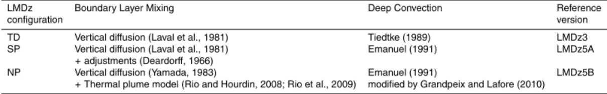
model (Rio and Hourdin, 2008; Rio et al., 2009) and the Emanuel (1991) convection scheme revisited by Grandpeix and Lafore (2010) with a new triggering and closure for-mulation and the representation of cold pools driven by the evaporation of precipitation. This configuration is very similar to LMDz5B (Hourdin et al., 2013b), which has been used to produce a set of CMIP5 simulations with IPSL-CM5B. We use “TD” to refer 25

(10)

GMDD

7, 4993–5048, 2014

R. Locatelli et al.

Title Page

Tables Figures

◭ ◮

Back Close

Full Screen / Esc

Discussion

P

a

per

|

Discus

sion

P

a

per

|

Discussion

P

a

per

|

Discussion

P

a

per

version of LMDz (hereafter named “SP” standing for Standard Physic), which uses the Emanuel (1991) scheme for convection, but not the thermals, and also differs from TD in the boundary layer mixing (a counter-gradient term on potential temperature is added according to Deardorff, 1966). This last configuration is the LMDz5A version used for CMIP5 simulations with IPSL-CM5A and is very close to the original LMDz4 5

version (Hourdin et al., 2006). Unless otherwise specified, all versions of LMDz are run with 96x96 points in both horizontal directions, and with 39 vertical layers. A summary of model versions is presented in Table 1.

3 Evaluation of atmospheric transport in the PBL

In this section, we investigate the ability of the LMDz model to represent transport of 10

tracers in the planetary boundary layer, first at one dimension (Sect. 3.1) and then with the 3-D model (Sect. 3.2).

3.1 LMDz Single Column Model vs. Large Eddy Simulation

In recent decades, several comparisons have been made between Single Column Models (SCM) and Large Eddy Simulations (LES) to better understand physical pa-15

rameterisations (Ayotte et al., 1996; Galmarini, 1998).

Here we compare three single-column versions of LMDz with LES from the non-hydrostatic model Meso-NH (Lafore et al., 1998). Originally, these LES were designed to evaluate the conditional sampling used by Couvreux et al. (2010) for the improve-ment of convective boundary layer mass-flux parameterisations. Here, we use them 20

(11)

GMDD

7, 4993–5048, 2014

R. Locatelli et al.

Title Page

Tables Figures

◭ ◮

Back Close

Full Screen / Esc

Discussion

P

a

per

|

Discus

sion

P

a

per

|

Discussion

P

a

per

|

Discussion

P

a

per

tracer is emitted every minute with a constant surface flux, and has a first-order decay time constant of 15 min. The horizontal LES resolution is 40 m and there are 40 verti-cal levels between the surface and 4000 metres. We consider the LES as our point of reference.

The three versions of LMDz-SCM used are differentiated by their deep convection 5

and vertical diffusion parameterisations. Firstly, SCM-TD uses the Tiedtke (1989) deep convection scheme, while SCM-SP uses the Emanuel (1991) deep convection scheme. Both of these versions use a local formulation of the turbulence to represent small-scale mixing. In the following we also refer to Emanuel (1991) scheme using “KE” abbreviation. Secondly, SCM-NP contains the most recent physical parameterisations 10

introduced in LMDz (thermal plume model of Rio and Hourdin, 2008; Rio et al., 2009 combined with Yamada, 1983 vertical diffusion). In SCM-TD and SCM-SP, the deep convection scheme is meant to represent both shallow and deep convection so that the Tiedtke and Emanuel schemes have to be activated to represent this case of fair-weather cumulus. However, in SCM-NP, shallow convection is handled by the thermal 15

plume model and the Emanuel scheme is deactivated in this simulation.

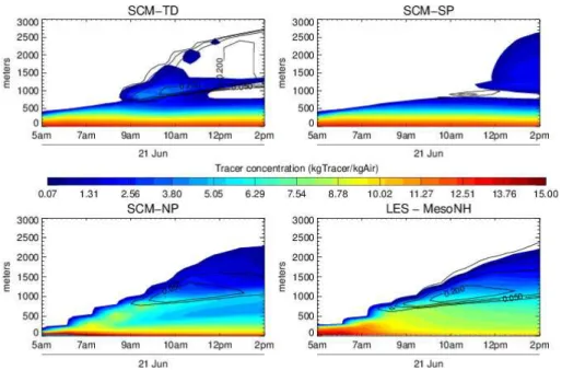
During the 9 h LES (Fig. 1, bottom right), the usual boundary layer thickening is observed during the morning related to incoming solar radiation. Physical processes acting in the boundary layer (small-scale turbulence, convection, mixing by thermal plumes, etc.) vertically distribute the surface-emitted tracer. At 1:00 p.m. LT (Local 20

Time), the tracer is diluted within a layer reaching 2000 metres.

The three LMDz-SCM versions exhibit markedly different skills in their attempt to re-produce the LES reference case. In the SCM-TD and SCM-SP simulations, the tracer is confined within a 500 m layer near the surface until 9 a.m. LT (SCM-TD) or 12 p.m. LT (SCM-SP). In SCM-TD, some tracer mass is transported vertically after 9 a.m. LT, but 25

tracer concentrations in the upper layers stay much lower than in the LES case. Indeed, tracer mixing ratios are insignifiant at 2000 m after 11 a.m., while they reach 3.5 kg kg−1

(12)

GMDD

7, 4993–5048, 2014

R. Locatelli et al.

Title Page

Tables Figures

◭ ◮

Back Close

Full Screen / Esc

Discussion

P

a

per

|

Discus

sion

P

a

per

|

Discussion

P

a

per

|

Discussion

P

a

per

LES. In particular, surface mixing ratios are largely over-estimated (9 kg kg−1 _{in the}

LES vs. 13 kg kg−1 _{in SCM-SP). These statements suggest that vertical mixing during}

a shallow convection case are badly represented in SCM-TD and SCM-SP. By contrast, SCM-NP shows better agreement with the LES reference: the tracer is vertically mixed in a layer that is thickening during the day as in the reference. Given that the KE scheme 5

was deactivated in the SCM-NP simulations, in order to highlight thermal actions on vertical mixing, it appears that thermals and vertical diffusion are responsible for the good representation of atmospheric transport in this case of shallow convection. How-ever, it is also important to note that tracer mixing ratios are slightly under-estimated in the mixed layer. It is especially true at 12 p.m. around 500 m: SCM-NP simulates tracer 10

mixing ratios of 5 kg kg−1_{, while they reach 8 kg kg}−1 _{in the LES. The underestimation}

of tracer concentrations in the mixed layer could be due to an underestimation of de-trainment from thermals at those levels or to the underestimation of vertical mixing by the diffusive scheme.

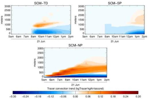
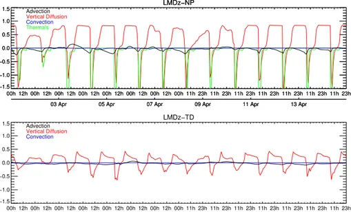
We hereafter define trends as the change of mixing ratios (or activity for 222Rn, 15

Sect. 3.2.2) due to a certain transport process (unit: mass mixing ratio (or Bq m−3 _for

222

Rn) per a unit of time; processes: PBL mixing, convection, thermals and advection). Here, the unit is kilogram per kilogram per second (kg kg−1_s−1_{). Trends in the vertical}

transport of tracers in the boundary layer due to deep convection (TD and SCM-SP) and thermal plumes (SCM-NP) are shown in Fig. 2. Positive trends (red colours) 20

at a specific level mean that the process brings tracer to this level. Conversely, nega-tive trends (blue colours) mean that the process moves some tracer to another level. In SCM-TD and SCM-SP, vertical transport of the tracer within the PBL (after 9 a.m. and 12 p.m. respectively) is not due to the PBL and turbulent diffusion scheme but, in an opportunistic way, to deep convection (Fig. 2, top left and top right). In SCM-NP, 25

(13)

GMDD

7, 4993–5048, 2014

R. Locatelli et al.

Title Page

Tables Figures

◭ ◮

Back Close

Full Screen / Esc

Discussion

P

a

per

|

Discus

sion

P

a

per

|

Discussion

P

a

per

|

Discussion

P

a

per

to simulate convection reaching only 2000 m height, whereas the modelling of atmo-spheric transport within cumulus-topped convective boundary layer is well reproduced by the thermal scheme (Rio and Hourdin, 2008). This case of the atmospheric trans-port of a short-lived tracer confirms that the thermal plume model of Rio and Hourdin (2008); Rio et al. (2009) is really efficient at properly simulating shallow convective 5

mixing over land.

3.2 Three dimensional simulations of222Rn

3.2.1 Statistical evaluation in the PBL

After a promising 1-D evaluation (Sect. 3.1), we seek here to evaluate the new physical parameterisations of LMDz for 3-D simulations on longer time and spatial scales. To 10

do so, we used the different versions of LMDz (Table 1) to simulate concentrations of the natural radioactive gas radon (222Rn). Radon is particularly well suited to evaluate diurnal mixing in the continental lower troposphere because it is a poorly soluble gas, and it is only emitted by continental surfaces and has a half-life of 3.8 days. These physical characteristics have lead radon to be used in many studies evaluating the per-15

formance of GCMs (Mahowald et al., 1997; Genthon and Armengaud, 1995; Belikov et al., 2013). Radon is produced from the radioactive decay of uranium-238 and is emit-ted fairly uniformly from terrestrial surfaces. Generally, radon emissions are quite well known globally (Zhang et al., 2011), and it is considered that a flux of 1 atom cm−2_s−1

is approximately valid for ice-free terrestrial surfaces (Jacob et al., 1997). While con-20

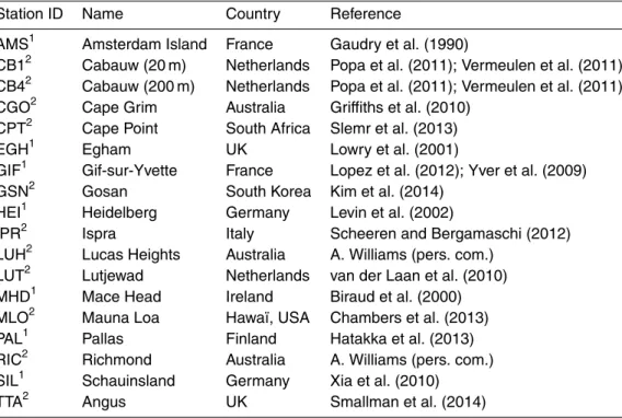
tinuous radon measurements exist worldwide, the coverage is better in Europe. There-fore, here we use a refined radon flux map for European emissions (Karstens et al., 2014), the rest of the continental lands emitting 1 atom cm−2_s−1_{between 60 and 60}◦_S

and 0.5 atom cm−2_s−1 _{between 60 and 70}◦_{N (excluding Greenland). Elsewhere, no}

radon flux is considered. As a consequence, our analysis is focused mainly on Euro-25

(14)

GMDD

7, 4993–5048, 2014

R. Locatelli et al.

Title Page

Tables Figures

◭ ◮

Back Close

Full Screen / Esc

Discussion

P

a

per

|

Discus

sion

P

a

per

|

Discussion

P

a

per

|

Discussion

P

a

per

measurements are available for this study. Note that different measurement techniques are used at the stations to measure222Rn. In particular, 222Rn measurements using methods based on short-lived daughters applied a station depended disequilibrium factor (Schmithüsen, 2014).

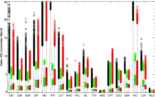
Figure 3 provides a statistical overview of the performance of the NP and TD mod-5

els by comparing measured and simulated hourly radon concentrations over a 6 year period (2006–2011). Here the red boxplots represent the NP simulations, whereas the green boxplots correspond to simulations using the current version of LMDz in PYVAR (the TD simulation). The black boxplots represent the observations.

For most stations, the box width (representing the interquartile range) is relatively 10

similar between observed and simulated values. However, large di_fferences occur in the extreme values (black circles). The observed high concentration “outliers” correspond primilarly to pre-dawn measurements on stable nights when PBL heights are lowest. A considerably better agreement is generally found between observed outliers and those simulated by NP, meaning that the NP simulation is better at representing the 15

shallow nocturnal PBL mixing depths associated with stable atmospheric conditions. Nocturnal mixing depths in TD, on the other hand, are too deep when the atmosphere is stable, or nearly stable, resulting in considerable underestimation of the outlier radon values.

More precisely, skills of TD and NP simulations may be very di_fferent at some specific 20

stations. For example, NP simulation gives remarkably good results at Heidelberg (HEI) station where NP is able to reproduce the strong diurnal cycle of222Rn concentrations measured at this site. On the contrary, TD time series at Heidelberg are very smooth and the diurnal cycle amplitude is strongly under-estimated. Similar results are found at Richmond (RIC) station in Australia. At Ispra (IPR) station, both TD and NP models dis-25

(15)

GMDD

7, 4993–5048, 2014

R. Locatelli et al.

Title Page

Tables Figures

◭ ◮

Back Close

Full Screen / Esc

Discussion

P

a

per

|

Discus

sion

P

a

per

|

Discussion

P

a

per

|

Discussion

P

a

per

of LMDz, for this complex location. This is a typical example of representativity errors in global models.

3.2.2 Case studies in the PBL

Here, we illustrate some typical LMDz behaviours in two case studies: at Heidelberg (Germany) in April 2009 (Figs. 4 and 5) and Lutjewad (Netherlands) in February 2008 5

(Figs. 6 and 7).

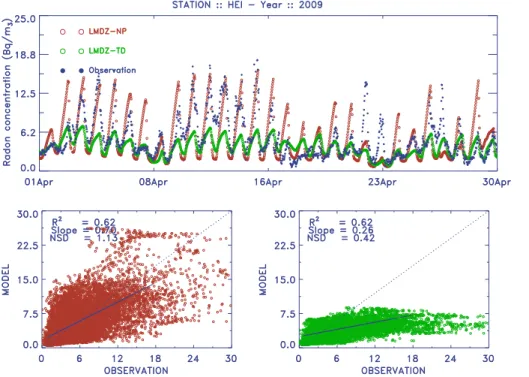
At Heidelberg in April 2009 (Fig. 4), NP reproduces the radon diurnal cycle very well, especially the peak nocturnal concentrations between the 8 and the 16 April. TD, on the other hand, poorly reproduces the amplitude of the diurnal cycle; with peak nocturnal values (7 Bq m−3_{) reaching less than half of the observed peaks (18 Bq m}−3_).

10

As a consequence, for the whole month of April, normalized standard deviations (NSD) are much better for NP (1.13) than for TD (0.42).

To better understand the contrasting behaviour of the two LMDz versions here, we compare time series of process trends for the first half of April 2009 at Heidelberg (Fig. 5). Trends are expressed here in Bq m−3_h−1_{. Similar trend daily cycles are clearly}

15

evident for each process. Vertical diffusion trends are positive from 18:00 to 08:00 UTC in NP. Indeed, with low nocturnal PBL height, vertical diffusion processes distribute the surface emitted radon throughout only a shallow layer resulting in a strong accumu-lation of radon near the surface. Vertical diffusion trends then become negative until 14:00 UTC. The PBL starts to grow in the morning, with the increase in solar radiation, 20

and radon accumulated near the surface over the previous night is mixed with low radon air from higher levels, resulting in lower sampled radon concentrations and a negative vertical diffusion trend. When radon is well-mixed throughout the PBL by vertical dif-fusion processes, the vertical di_ffusion trend becomes positive again, since radon is emitted at the surface. The thermals scheme transports high levels of radon from the 25

(16)

GMDD

7, 4993–5048, 2014

R. Locatelli et al.

Title Page

Tables Figures

◭ ◮

Back Close

Full Screen / Esc

Discussion

P

a

per

|

Discus

sion

P

a

per

|

Discussion

P

a

per

|

Discussion

P

a

per

trend is null), and the impact of advection on radon concentration at Heidelberg station is generally insignificant.

For TD, the vertical diffusion trend is relatively similar to NP, although the magnitude of its diurnal cycle is 60 % smaller. Indeed, maximum (minimum) of vertical diffusion trend does not exceed 0.4 Bq m−3_h−1 ₍

−0.5 Bq m−3h−1, respectively), while it reaches

5

0.8 Bq m−3_h−1 ₍

−1.5 Bq m−3h−1) in the NP simulation. In TD, the vertical diffusion is

generally acting in a thicker layer, so the accumulation of radon close to surface is less pronounced, leading to smaller vertical diffusion trends. As was the case for NP, convection and advection processes are insignificant for TD, which contains no ther-mals. Despite the differences noted above, R-squared statistics are equal in NP and 10

TD (0.62 for the two simulations) for Heidelberg in April 2009 (Fig. 4 bottom). One factor contributing to R-square values for NP lower than expected was that NP occa-sionally simulated peaks that were not observed as evident in Fig. 4 toward the end of April 2009, which fastly degrades the R-square statistic in the NP case.

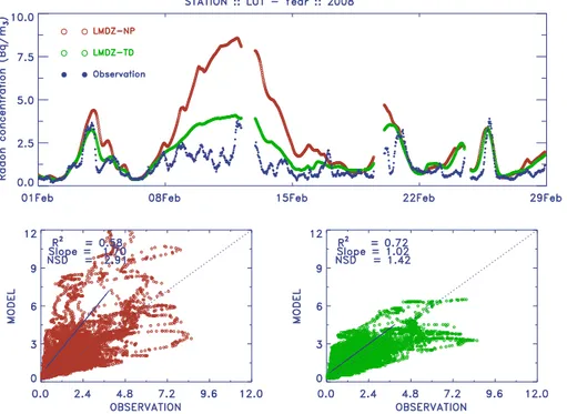
We now investigate this issue with the example of radon time series at Lutjewad in 15

February 2008 (Fig. 6). Indeed, a peak reaching 9 Bq m−3_{(4 Bq m}−3_{) is simulated by NP}

(TD respectively) between the 8 and the 15 February, while smaller peaks are observed (around 3 Bq m−3_{). However, the analysis of physical process trends at Lutjewad for the}

same period (Fig. 7) is relatively similar to Heidelberg’s analysis. To understand this apparent inconsistency, an analysis of near-surface quantities has been performed. 20

When two-metre temperatures (T2 M) simulated by TD and NP are compared with those obtained from the ERA-Interim product (not shown here), it is found that they are quite di_fferent (up to 7◦_{) during the month of February 2008. Consequently, the PBL heights}

are probably very different between the models and the reanalysed data, and one can not expect any good scores for modelling of radon transport to Lutjewad during this 25

(17)

GMDD

7, 4993–5048, 2014

R. Locatelli et al.

Title Page

Tables Figures

◭ ◮

Back Close

Full Screen / Esc

Discussion

P

a

per

|

Discus

sion

P

a

per

|

Discussion

P

a

per

|

Discussion

P

a

per

We have also looked at surface characteristics for the Heidelberg case. Both sim-ulations are able to reproduce diurnal cycle of T2 M given by ERA-Interim product in April 2009. However, only222Rn simulated by NP is able to fit the strong222Rn diurnal cycle measured at Heidelberg in April 2009. This confirms again that responses in TD simulations are much smoother than in NP simulations.

5

4 Modelling of large-scale atmospheric transport

In this section, we investigate the ability of different LMDz versions to represent large-scale (e.g. inter-hemispheric or troposphere/stratosphere) trace gas exchanges. To do so, we focus on longer-lived species, such as the inert sulfur hexafluoride (SF6) (Sects. 4.1, 4.2.1 and 4.3) or carbon dioxide (CO2) (Sect. 4.2.2), and reactive methane 10

(CH₄) (Sect. 4.4).

4.1 Large-scale transport features of LMDz configuration using SF6simulations

SF6 is a trace gas used in equipment for electrical transmission and distribution sys-tems and in the reactive metals industry (Maiss and Brenninkmeijer, 1998). It has been widely used to study atmospheric transport (Denning et al., 1999; Law et al., 2008; 15

Patra et al., 2009). Since it is inert, SF6is very long-lived in the troposphere and strato-sphere (between 800 to 3200 years; Ravishankara et al., 1993; Morris et al., 1995), which makes SF₆a powerful tool for assessing large-scale modelling of transport pro-cesses in the atmosphere (Maiss et al., 1996).

Here we employ monthly zonal averages of SF6to investigate boundary layer mixing 20

(mixing due to vertical di_ffusion in TD and SP, and mixing due to both vertical di_ffusion and thermal plumes in NP), convection and advection (unit is mass mixing ratio per month (pptm month−1_{)) as modelled in LMDz for three di}

(18)

GMDD

7, 4993–5048, 2014

R. Locatelli et al.

Title Page

Tables Figures

◭ ◮

Back Close

Full Screen / Esc

Discussion

P

a

per

|

Discus

sion

P

a

per

|

Discussion

P

a

per

|

Discussion

P

a

per

(July, see Fig. 8) as convection intensity over locations where SF₆ is mainly emitted (between 30 and 60◦_{N) is maximum during summer.}

First of all, we detail the general transport pathway for the three configurations of LMDz. Vertical diffusion (including thermal plumes in NP) mixes SF₆ from the sur-face throughout the boundary layer (Fig. 8, top). This is very clear between 30 and 5

60◦_{N where SF}

6emissions are stronger. Above the boundary layer, vertical diffusion gradually reduces and vertical transport is mainly accomplished by deep convection (Fig. 8, middle), which moves SF6 from the boundary layer to the top of the tropo-sphere (∼200 hPa). The large positive convection trend area between 30 and 60◦N is

consistent with the location of both strong convection area over continents and strong 10

SF₆ emissions at this period of the year. Then, tropospheric SF₆ is advected from 30–60◦_{N to 15}◦_S–15◦_{N band by meridional advection (Fig. 8, bottom). Finally, SF}

6is transported from the high to the low levels of the troposphere by subsident motions forming the descending branch of the Hadley cell between 15S and 5N (blue plume on Fig. 8, middle).

15

General characteristics of large-scale transport look similar between model versions but one can wonder how much the three configurations of the model (NP, TD and SP) differ. Looking at the transport in the boundary layer, the main difference is the height at which mixing due to vertical diffusion (and thermals for NP configuration) transports SF₆. In TD or SP, vertical di_ffusion processes transport SF₆up to 600 hPa, while in NP 20

SF6 is transported slightly higher, up to 500 hPa. If one splits the processes acting in the boundary layer for the NP configuration, one finds that vertical diffusion is mainly active from surface to 900 hPa and thermals are responsible for SF₆transport in higher parts of the boundary layer as has been shown in Sect. 3.1. Moreover, when using the Tiedtke (1989) scheme (TD), convection transports SF6across more layers than in the 25

(19)

GMDD

7, 4993–5048, 2014

R. Locatelli et al.

Title Page

Tables Figures

◭ ◮

Back Close

Full Screen / Esc

Discussion

P

a

per

|

Discus

sion

P

a

per

|

Discussion

P

a

per

|

Discussion

P

a

per

convection trends over 40◦_{N in NP and SP that the intensity of convection is weaker}

when the thermal plume model is activated, which can be expected.

4.2 IH exchange with SF6and biospheric-CO2simulations

4.2.1 SF6simulations

The IH exchange of trace gases simulated by CTMs is very valuable indicators of 5

how atmospheric transport performs at the global scale. For example, Patra et al. (2011) compare the IH exchange time simulated by di_fferent CTMs with an indirectly-measured exchange time using SF6 measurements. Their method use SF6 measure-ments at two stations of the Northern Hemisphere (Barrow (Alaska, USA) and Mauna Loa (Hawaï, USA) stations) and two stations of the Southern Hemisphere (Cape Grim 10

(Australia) and South Pole stations) to derive the IH gradient. We tried to apply this method in our study. However we found that uncertainties related to the choice of sta-tions and to the station sampling levels appeared to be larger than di_fferences in IH exchange time simulated by the different configurations of LMDz. Consequently, we do not further discuss the IH exchange time, but we analyze the IH exchange by studying 15

SF₆meridional gradients.

Annual means of SF6surface mole fractions, zonally averaged and at 11 measure-ment sites, are plotted in Fig. 9a for five different configurations of LMDz. This view of the north-to-south SF₆ surface gradient gives a direct indication of IH exchange. The NP, SP and TD configurations (96×96×39) of LMDz are shown in red, blue and

20

green respectively. We have also investigated the impact of a higher horizontal (TD-144×142×39, purple line) and a lower vertical (TD-96×72×19, orange line) resolution

on IH exchange. The black diamonds show the measured SF6mole fraction at different surface stations. The coloured crosses show the station value for the different model configurations. For better clarity, the results of the different simulations have been ad-25

(20)

GMDD

7, 4993–5048, 2014

R. Locatelli et al.

Title Page

Tables Figures

◭ ◮

Back Close

Full Screen / Esc

Discussion

P

a

per

|

Discus

sion

P

a

per

|

Discussion

P

a

per

|

Discussion

P

a

per

Knowing that the majority of SF₆emissions are located in the Northern Hemisphere, it is not surprising to see SF6mole fraction shifting from 5.49 ppt at the South Pole to 5.81 ppt at Alert (Canada). The maximum of zonal mean SF6mole fraction is reached at around 40◦_{N, close to the latitudes of maximum emissions. Figure 9a shows that}

simulated SF6mole fractions in all LMDz configurations over-estimate (under-estimate) 5

SF6 measurements in the high latitudes of the Southern Hemisphere (in the very high latitudes of the Northern Hemisphere) confirming that IH exchange is too fast in LMDz (Patra et al., 2011). However, the two configurations of LMDz, SP and NP, both using the deep convection scheme of Emanuel (1991), have a slightly steeper IH gradient (∼8 %), although still smaller than the observed IH gradient. The steeper vertical

gra-10

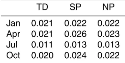
dient in the lower part of the troposphere when using the Emanuel scheme could be an explanation. Indeed, the detrainment in the Emanuel (1991) scheme was smaller between 800 and 600 hPa (Sect. 4.1) compared to the Tiedtke (1989) scheme. This leads to slightly higher vertical gradient in the lower part of the troposphere as shown in Table 3, which summarizes the vertical gradient of SF6between 900 and 500 hPa for 15

the different physical sets of parameterisations used in LMDz. This is consistent with Saito et al. (2013) who show that latitudinal gradients in a CTM are generally propor-tional to the vertical gradients in the lower troposphere. Furthermore, vertical transport by thermals reduces vertical gradient in NP compared to SP in the first layers of the troposphere, which may explain the slightly smaller IH gradient computed in NP com-20

pared to SP. Furthermore, we find similar IH gradients when using different vertical and/or horizontal resolution with the TD version of LMDz. On the contrary, Patra et al. (2011) found slight di_fferences between IH exchange time of high and low horizontal resolution versions of two CTMs. However, the gap between the high and the low hori-zontal resolutions (from 6◦

×4◦to 1◦×1◦and from 5◦×4◦to 1.25◦×1◦) of the CTMs used

25

in their study is much larger that the gap used here (from 1.875◦

×3.75◦to 1.25◦×2.5◦).

(21)

GMDD

7, 4993–5048, 2014

R. Locatelli et al.

Title Page

Tables Figures

◭ ◮

Back Close

Full Screen / Esc

Discussion

P

a

per

|

Discus

sion

P

a

per

|

Discussion

P

a

per

|

Discussion

P

a

per

gradients simulated by different CTMs exhibit differences up to 0.2 ppt. This suggests that modifications in sub-grid scale parameterisations of LMDz causes only small dif-ferences in IH transport characteristics for SF6.

4.2.2 Biospheric-CO2simulations

Meridional transport may not be the only cause for IH gradient of trace gases. Indeed, 5

the so-called rectifier effect, introduced by Denning et al. (1995), is one cause for the existence of meridional gradient of biospheric CO2mole fraction. The seasonal rectifier effect is the consequence of the correlation between the atmospheric transport in the PBL and the surface biospheric CO2flux. Indeed, both atmospheric turbulence and the flux of CO2from the biosphere to the atmosphere undergoes a seasonal cycle. During 10

winter, at mid to high latitudes, microbial respiration dominates photosynthesis leading to net CO2emissions to the atmosphere. Moreover, stable atmospheric conditions are predominant in winter. It results higher CO2 mole fractions at the surface than if no correlation occurs. On the contrary, during summer, photosynthesis is dominating upon respiration and unstable atmospheric conditions prevail, leading to the dilution of the 15

net flux from atmosphere to land by strong turbulence. In summer, PBL depth can reach 2 km above mid-latitude continents at midday (Seidel et al., 2012). It results lower mole fractions at the surface than if no correlation occurs. Consequently, on an annual basis, even if global biospheric CO2emissions are set to zero, a meridional gradient can be generated with higher mole fractions in the Northern Hemisphere than in the Southern 20

Hemisphere, especially above northern continental regions, such as Siberia (Denning et al., 1995).

The Fig. 9b exposes the impact of this rectifier effect on the meridional CO2gradient by showing surface zonal annual mean CO₂mole fraction due to biosphere emissions only, with zero annual emissions, as simulated by three configurations of LMDZ (NP, 25

(22)

GMDD

7, 4993–5048, 2014

R. Locatelli et al.

Title Page

Tables Figures

◭ ◮

Back Close

Full Screen / Esc

Discussion

P

a

per

|

Discus

sion

P

a

per

|

Discussion

P

a

per

|

Discussion

P

a

per

Pole. These gradients are in agreement with what was previously found on the recti-fier effect in the TransCom experiment (Law et al., 1996; Gurney et al., 2003). Indeed, the range of meridional biospheric CO2 gradient among chemistry-transport models spread from 0 to 3.5 ppm both in Law et al. (1996) and Gurney et al. (2003). In Law et al. (1996), model results can be clustered in two groups: one group of models sim-5

ulating seasonal rectifier around 0.5 ppm and one other group with rectifier around 2 ppm. In Gurney et al. (2003), simulated rectifier effects are much more spread be-tween 0 and 3 ppm. From these two studies, one can conclude that NP simulating a rectifier effect of 1.8 ppm is in the higher part of the range since only 4 CTMs (over a total of 17 different CTMs) simulate a stronger rectifier effect. On the contrary, TD 10

simulating a rectifier e_ffect of 1.0 ppm is in the lower part since only 6 CTMs simulate a weaker rectifier effect.

Furthermore, it is noticeable to see that the different configurations of LMDz simu-late oscillations in CO₂ mole fraction around 5◦_{N (Fig. 9b), which is a consequence}

of the correlation between the seasonal shift of the Intertropical Convergence Zone 15

(ITCZ) and biosphere flux in the Tropics. It is also interesting to note that LMDz-NP and LMDz-SP give similar results in the Tropics and large di_fferences from 45◦_{N. Knowing}

that LMDZ-NP and LMDZ-SP uses the same deep convection mixing scheme and that deep convection is the main contributor to vertical mixing in the Tropics, it is not sur-prising to have similar results in these regions. Howewer, in extra-tropics regions of the 20

Northern Hemisphere vertical diffusion and mixing due to thermals have a significant impact on biospheric CO2 mixing, especially over Siberia (not shown), where most of the rectifier applies in LMDz. Moreover, magnitudes of the physical trends due to ver-tical diffusion and thermals can be highly different between LMDz-NP and LMDz-SP at these latitudes, which can explain why these two configurations of LMDz simulate 25

significantly di_fferent rectifier e_ffects.

(23)

GMDD

7, 4993–5048, 2014

R. Locatelli et al.

Title Page

Tables Figures

◭ ◮

Back Close

Full Screen / Esc

Discussion

P

a

per

|

Discus

sion

P

a

per

|

Discussion

P

a

per

|

Discussion

P

a

per

directly measure rectifier effects (Yi et al., 2004; Chen et al., 2004; Stephens et al., 2013). Although these studies bring very valuable knowledge on the rectifier effect at local scales, they cannot allow to draw conclusions on the magnitude of the rectifier ef-fect at the global scale. In fact, Yi et al. (2004) compare the rectifier effect simulated by the CSU GCM (Colorado State University GCM) with observed rectifier forcing at a spe-5

cific station in northern Wisconsin (USA). They conclude that the observed seasonal covariance between ecosystem CO₂fluxes and PBL turbulent mixing are stronger than the same signals simulated by the CSU GCM. Chen et al. (2004) developed a Vertical Diffusion Scheme (VDS) to investigate the rectifier effect and validate their model with measurements at Fraserdale, Ontario, Canada. They conclude that the seasonal rec-10

tifier e_ffect contribute largely to the total rectifier e_ffect: 75 % of the total rectifier e_ffect is due to the seasonal rectifier effect, while the rest is caused by the diurnal rectifier effect. On the contrary, Stephens et al. (2007) argue for a weak seasonal rectifier effect (see Fig. 7 in Supplement of Stephens et al., 2007).

Finally, one can hardly conclude from these incomplete pieces of information which 15

version of LMDz better simulates the rectifier effect. However, these differences in the representation of the rectifier e_ffect will definitely have large impacts on inverse esti-mates (see Sect. 5). Moreover, large efforts have been recently done to provide a global PBL climatology based on observations (Seidel et al., 2012; McGrath-Spangler and Denning, 2013), which could also give valuable information on the PBL mixing. Thus, 20

from such approaches, an observation-driven estimation of the actual magnitude of the rectifier effect could emerge soon, which will be very interesting for future evaluation of CTMs.

4.3 Stratosphere/Troposphere exchange (STE) using long-lived species

Exchanges between the stratosphere and troposphere may have large impacts on at-25

(24)

GMDD

7, 4993–5048, 2014

R. Locatelli et al.

Title Page

Tables Figures

◭ ◮

Back Close

Full Screen / Esc

Discussion

P

a

per

|

Discus

sion

P

a

per

|

Discussion

P

a

per

|

Discussion

P

a

per

compare the atmospheric distribution of N₂O as simulated by different CTMs with a fo-cus on the representation of STE. They show that the Brewer–Dobson circulation is poorly simulated by LMDz, which badly resolves seasonal influence of STE on N2O mole fractions. In Patra et al. (2011), focusing on CH₄simulations, LMDz is also pointed out to simulate STE that is too fast compared to others CTMs with a wrong position of 5

the tropopause (especially in the Tropics). These results exhibited in Thompson et al. (2014) and Patra et al. (2011) have been obtained using the physical parameterisations of TD configuration and with a low vertical resolution (19 levels). These two studies clearly identify the low vertical resolution of LMDz as a factor responsible for the poor STE representation. Moreover, Hourdin et al. (2013a), studying the impact of LMDz grid 10

configuration on the climate, have shown that more vertical layers in the stratosphere leads to a better representation of stratospheric variability. Thus, one can hypothesize that by increasing the number of model layers from 19 to 39, with especially more lay-ers in the PBL and above the tropopause, the model will better simulate exchange at the transition between troposphere and stratosphere.

15

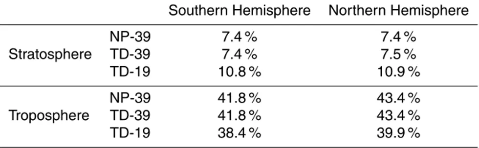
To investigate this statement, we present comparisons of SF6burden computed for 4 boxes (stratosphere and troposphere in northern and Southern Hemisphere) between two LMDz 39-layers versions (NP-39 and TD-39) and one LMDz version using only 19 vertical layers (TD-19). The limit between stratosphere and troposphere has been set at 150 hPa in all simulations. Knowing that SF₆ is very well-mixed in the troposphere 20

and in the stratosphere, one can evaluate STE efficiency by comparing the SF6burden (Table 4).

First of all, it is found that di_fferences between versions using di_fferent vertical res-olutions are much larger than differences between LMDz versions using same vertical resolution but different physical parameterisations. Indeed, it is found that 10.9 % of to-25

(25)

GMDD

7, 4993–5048, 2014

R. Locatelli et al.

Title Page

Tables Figures

◭ ◮

Back Close

Full Screen / Esc

Discussion

P

a

per

|

Discus

sion

P

a

per

|

Discussion

P

a

per

|

Discussion

P

a

per

Similar results are found for the Southern Hemisphere. Therefore exchange between the troposphere and stratosphere is slowed down with the 39-layers configuration of LMDz, which improves the flaw of LMDz regarding STE representation.

Moreover, we have computed the tropopause height using the method described in Reichler et al. (2003). Thus, the tropopause height is defined as the height at which the 5

temperature lapse rate becomes less than 2 K km−1_{. This is also the approach used}

in Thompson et al. (2014). We find that TD-19, TD-39, SP-39 and NP-39 simulate tropopause height in the Tropics at 109, 105, 106 and 106 hPa respectively, which is consistent with the results found in Thompson et al. (2014). Indeed, they computed the tropopause height for 8 CTMs and they found that the tropopause height ranged from 10

101 to 106 hPa for 7 CTMs, while the tropopause height computed using LMDz (TD-19 configuration) was an outlier since it reached 109 hPa. Consequently, by improving vertical resolution from 19 to 39 levels, the tropopause height simulated by LMDz falls into the range of 7 CTMs simulating quite well STE (Thompson et al., 2014). Moreover, we assess here also that modifications on vertical resolutions impact much more the 15

location of tropopause height that modifications on physical parameterisations.

Finally, these di_fferent results confirm that STE is improved in LMDz configurations using a finer vertical resolution (39 vs. 19 vertical levels).

4.4 Reactive species

Changes in the parameterisations of atmospheric processes in GCMs can also af-20

fect atmospheric chemistry (Mahowald et al., 1995). Indeed, Tost et al. (2010) have shown that the use of different sub-grid scale schemes affects atmospheric chemistry by changing both the meteorology (for example, modification of convection intensity) and chemistry (for example, modifications in location of the photochemical reactions). These different impacts on atmospheric chemistry cannot be tested with a passive 25

(26)

GMDD

7, 4993–5048, 2014

R. Locatelli et al.

Title Page

Tables Figures

◭ ◮

Back Close

Full Screen / Esc

Discussion

P

a

per

|

Discus

sion

P

a

per

|

Discussion

P

a

per

|

Discussion

P

a

per

oxidized by hydroxyl radical (OH) in the troposphere (Kirschke et al., 2013). We ran simulations with the different configurations of LMDz to test this question.

Figure 10 shows 39 years of daily CH4 mole fraction averaged at global scale and over the first layers of the atmosphere (between surface and 850 hPa) for TD, NP and SP configurations. The exact same setup is used for these simulations (climatological 5

CH4 emissions of 500 Tg CH4year− 1

, climatological oxidant fields and surface initial mean mole fraction of 1650 ppb). In the three simulations, the time series of CH₄mole fraction exhibit typical seasonal cycles each year with a low during boreal summer and a high during boreal winter. Simulated seasonal cycles are very consistent between the three LMDz configurations. As emissions and sinks are climatological, CH₄global mole 10

fraction tends to reach a steady state. Indeed, TD and SP simulations annual CH₄mole fraction tend to reach 1778 and 1775 ppb respectively after 30 years of simulations. The NP version, however, diverges from the SP and TD versions, with a steady state value of 1801 ppb being reached, around 25 ppb higher than TD and SP configurations. The use of different deep convection schemes could be responsible for such differences in 15

CH4state equilibrium. Indeed, Lelieveld and Crutzen (1994) have shown the significant role of deep convection on the ozone tropospheric budget. However, as the TD and SP configurations give similar results, one can infer that in this study the difference is due to the implementation of the thermal plume model, which contributes to perturbing the chemical equilibrium of CH₄. In other words, the methane lifetime increases when the 20

thermal plume scheme is activated. This increase has been assessed to be 0.2 years (2 % of the typical methane lifetime, Naik et al., 2013).

We further investigate the di_fference between NP/SP and TD CH₄ mole fractions. The chemical loss of methane is the product of a reaction ratekCH₄, OH concentrations and CH4 mole fraction. After investigation, we found that the difference of chemical 25

(27)

GMDD

7, 4993–5048, 2014

R. Locatelli et al.

Title Page

Tables Figures

◭ ◮

Back Close

Full Screen / Esc

Discussion

P

a

per

|

Discus

sion

P

a

per

|

Discussion

P

a

per

|

Discussion

P

a

per

temperature bias found in NP compared to SP and TD, as already shown in Hourdin et al. (2006), leads to a smaller consumption of methane by OH in the mid-troposphere for NP compared to SP and TD. In response, CH4steady-state mole fraction is higher in the NP configuration. Furthermore, this effect is amplified since the difference between the reaction rate for NP and TD is maximum around 700 hPa, where OH mole fractions 5

are also maximum.

5 Conclusions and implications for inverse modelling of trace gas emissions

and sinks

We have investigated the impacts of new physical parameterisations for deep con-vection (Emanuel, 1991) and boundary layer mixing due to vertical diffusion (Yamada, 10

1983) and thermal plumes (Rio and Hourdin, 2008; Rio et al., 2009) recently imple-mented in the LMDz GCM on atmospheric transport and chemistry of different trace gases. First, a comparison between a one-dimensional version of LMDz and a Large Eddy Simulation of Meso-NH shows that the atmospheric transport of a short-lived tracer is greatly improved by the activation of the thermal plume model in a case of shal-15

low convection over land. The combination of the deep convection scheme (Tiedtke, 1989) and vertical diffusion parameterisations (Laval et al., 1981) used in previous version of LMDz does not produce satisfactory results in the modelling of a growing boundary layer. Three dimensional simulations of222Rn, a tracer of surface continental air masses, confirm an overall improvement in PBL dynamics when the new parame-20

terisations for vertical diffusion and thermal plumes are implemented. In particular, the amplitude and phase of the diurnal radon signal is found to be much better reproduced when the thermal plume scheme is used. However, the higher variability of concentra-tions in NP simulaconcentra-tions increase the sensitivity of the results to external meteorological forcings.

25

(28)

GMDD

7, 4993–5048, 2014

R. Locatelli et al.

Title Page

Tables Figures

◭ ◮

Back Close

Full Screen / Esc

Discussion

P

a

per

|

Discus

sion

P

a

per

|

Discussion

P

a

per

|

Discussion

P

a

per

LMDz will allow us to assimilate a larger fraction of the high-frequency data (daily, and maybe hourly) sampled at surface stations located close to source areas, which often show large peaks of concentrations on hourly to weekly timescales. Such data not well simulated by the previous version of LMDz-SACS and therefore are either removed or associated with a very large uncertainty in the inverse procedure. However, the higher 5

sensitivity of NP version to the external forcing (see Sect. 3.2.2) may cause inadequate optimized fluxes if observation errors integrated into the inverse system are not consis-tently estimated. Indeed, one outcome of this work is that the transport model part of the observation error used for one observation in the inversion can largely depend on the configuration of the model used. Furthermore, a comparison of observation errors 10

integrated into three di_fferent inverse systems for methane flux estimation has shown that observation errors are often under-estimated which exacerbate the impact of trans-port model errors on optimized fluxes (Locatelli et al., 2013). Thus, it will be essential to put a lot of attention on the estimation of observation errors when configuring PYVAR inversion system with the new version of LMDz model.

15

The skill of LMDz to represent large-scale transport has also been studied using a long-lived trace gas (SF₆). General transport pathways show similar behaviours be-tween the different configurations of LMDz studied here. However, a few differences are noticeable. First, it is shown that use of the Emanuel deep convection scheme results in a small increase in the IH SF₆ gradient, although the gradient simulated by the NP 20

version of LMDz is still too weak compared to observations. Moreover, the combination of thermal plume model with the Emanuel scheme in LMDz-NP leads to a stronger rec-tifier e_ffect compared to LMDz-TD. Second, the stratosphere–troposphere exchange is largely improved by an increase in the vertical resolution (from 19 to 39 layers). Third, the thermal plume model plays an indirect role on the atmospheric loss of reactive 25