ACPD
9, 9367–9398, 2009Analysing spatio-temporal patterns of the global
NO2-distribution
M. Hayn et al.
Title Page
Abstract Introduction
Conclusions References
Tables Figures
◭ ◮
◭ ◮
Back Close
Full Screen / Esc
Printer-friendly Version
Interactive Discussion Atmos. Chem. Phys. Discuss., 9, 9367–9398, 2009
www.atmos-chem-phys-discuss.net/9/9367/2009/ © Author(s) 2009. This work is distributed under the Creative Commons Attribution 3.0 License.
Atmospheric Chemistry and Physics Discussions
This discussion paper is/has been under review for the journalAtmospheric Chemistry and Physics (ACP). Please refer to the corresponding final paper inACPif available.
Analysing spatio-temporal patterns of the
global NO
2
-distribution retrieved from
GOME satellite observations using a
generalized additive model
M. Hayn1, S. Beirle2, F. A. Hamprecht3, U. Platt4, B. H. Menze3,5,*, and T. Wagner2,*
1
Institut f ¨ur Mathematik, University of Potsdam, Potsdam, Germany
2
MPI for Chemistry, Mainz, Germany
3
ACPD
9, 9367–9398, 2009Analysing spatio-temporal patterns of the global
NO2-distribution
M. Hayn et al.
Title Page
Abstract Introduction
Conclusions References
Tables Figures
◭ ◮
◭ ◮
Back Close
Full Screen / Esc
Printer-friendly Version
Interactive Discussion
4
Institut f ¨ur Umweltphysik, University of Heidelberg, Heidelberg, Germany
5
Computer Science and Artificial Intelligence Lab, Massachusetts Institute of Technology, Cam-bridge, MA, USA
∗contributed equally
Received: 20 March 2009 – Accepted: 23 March 2009 – Published: 9 April 2009
Correspondence to: M. Hayn ([email protected])
ACPD
9, 9367–9398, 2009Analysing spatio-temporal patterns of the global
NO2-distribution
M. Hayn et al.
Title Page
Abstract Introduction
Conclusions References
Tables Figures
◭ ◮
◭ ◮
Back Close
Full Screen / Esc
Printer-friendly Version
Interactive Discussion Abstract
With the increasing availability of observations from different space-borne sensors, the joint analysis of observational data from multiple sources becomes more and more at-tractive. For such an analysis – oftentimes with little prior knowledge about local and global interactions between the different observational variables available – an explo-5
rative data-driven analysis of the remote sensing data may be of particular relevance. In the present work we used generalized additive models (GAM) in this task, in an exemplary study of spatio-temporal patterns in the tropospheric NO2-distribution de-rived from GOME satellite observations (1996 to 2001) at global scale. We modelled different temporal trends in the time series of the observed NO2, but focused on iden-10
tifying correlations between NO2 and local wind fields. Here, our nonparametric mod-elling approach had several advantages over standard parametric models: While the model-based analysis allowed to test predefined hypotheses (assuming, for example, sinusoidal seasonal trends) only, the GAM allowed to learn functional relations between different observational variables directly from the data. This was of particular interest 15
in the present task, as little was known about relations between the observed NO2 dis-tribution and transport processes by local wind fields, and the formulation of general functional relationships to be tested remained difficult.
We found the observed temporal trends – weekly, seasonal and linear changes – to be in overall good agreement with previous studies and alternative ways of data anal-20
ysis. However, NO2observations showed to be affected by wind-dominated processes over several areas, world wide. Here we were able to estimate the extent of areas affected by specific NO2 emission sources, and to highlight likely atmospheric trans-port pathways. Overall, using a nonparametric model provided favourable means for a rapid inspection of this large spatio-temporal data set,with less bias than parametric 25
ACPD
9, 9367–9398, 2009Analysing spatio-temporal patterns of the global
NO2-distribution
M. Hayn et al.
Title Page
Abstract Introduction
Conclusions References
Tables Figures
◭ ◮
◭ ◮
Back Close
Full Screen / Esc
Printer-friendly Version
Interactive Discussion 1 Introduction
Nitrogen oxides – NO and NO2, often referred to as NOx– belong to the most important atmospheric pollutants. NO2 is poisonous by inhalation (World Health Organization, 2003 and Elsayed, 1994) and NOx plays an important role in the atmospheric ozone budget (Jacob, 1999 and Seinfeld et al., 1997). NOxis influencing chemical and biolog-5
ical processes both locally (Uno et al., 1996 and Wakamatsu et al., 1998) and globally (Stohl et al., 2003 and Wenig et al., 2003), and its occurrence is closely related to human activities. Tropospheric NOxis a major contributor to tropospheric ozone smog in urban areas, and even at global scale a disproportionally high amount of the NOx originates from anthropogenic sources (Olivier et al., 1990 and Seinfeld et al., 1997). 10
With space-borne instruments, such as the Global Ozone Monitoring Experiment (GOME), global time series of NO2 and other tropospheric trace gases become in-creasingly available, with a considerable resolution both in time and space (ESA, 1995; Burrows et al., 1999; Bovensmann et al., 1999 and Wagner et al., 2008, Leue et al., 2001; Richter et al., 2002; Martin et al., 2002; Beirle et al., 2003; Beirle, 2004a,b and 15
Boersma et al., 2004). Also, with an increasing amount of observations from other space-borne sensors and high level products derived from them, such as e.g. global 3-dimensional wind fields, the joint analysis of observational data from multiple sources becomes more and more attractive. Here, with little prior knowledge about local and global interactions between the different observational variables available, an explo-20
rative data-driven analysis of the remote sensing data may be of particular relevance. A number of earlier studies focused on the global distribution of different tempo-ral patterns in the NO2 dynamics. Examples are the weekly cycle found to correlate well with anthropogenic sources (Beirle et al., 2003), the analysis of long term trends (Richter et al., 2005) and multi-component analyses (van der A et al., 2006 and van 25
ACPD
9, 9367–9398, 2009Analysing spatio-temporal patterns of the global
NO2-distribution
M. Hayn et al.
Title Page
Abstract Introduction
Conclusions References
Tables Figures
◭ ◮
◭ ◮
Back Close
Full Screen / Esc
Printer-friendly Version
Interactive Discussion In the present study we used a generalized additive model (GAM) (Hastie et al.,
1986 and Wood, 2006), which allows to include different components: a parametric linear trend, non-parametric annual and weekly cycles, and a term for the local wind fields. We chose GAM for two different purposes:
– First, to test the data for temporal trends which are more complex than the para-5
metric formulations used so far to study global trends of the NO2 distribution – similar to (Brillinger, 1994; Smith et al., 1999; Dominici et al., 2002; Aldrin et al., 2005; Kim et al., 2005 and Stige et al., 2006).
– Second, to model the relation between temporal dynamics of the observed NO2 and external observational variables, with as little assumptions as possible. This 10
allows us to consider local wind fields in the analysis of the temporal behaviour of the trace gas at a global level – to the best of our knowledge for the first time – and to uncouple local generation and transport of the observed NO2distributions.
The influence of this wind component is particularly high close to strong and continuous point sources like power plants or individual cities. Such regions are characterized by 15
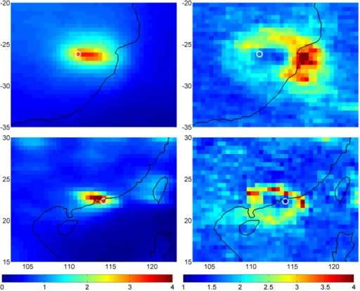
strong fluctuations of the tropospheric NO2concentration which can be easily identified e.g. by forming the ratio of the standard deviation and the median of the time series of the integrated tropospheric NO2concentration. High values of this ratio are e.g. found close to Hongkong and Johannesburg (see Fig. 1) and we will focus on those exam-ples to understand the contribution of local transport processes to the observed NO2 20
distributions.
In the following we describe the data used (Sect. 2) and the GAM adapted to our task (Sect. 3). We present global maps of spatial and temporal trends from the application of the model to the GOME data, and discuss the influence of the local wind field on the NO2trace gas dynamics observed (Sect. 4).
ACPD
9, 9367–9398, 2009Analysing spatio-temporal patterns of the global
NO2-distribution
M. Hayn et al.
Title Page
Abstract Introduction
Conclusions References
Tables Figures
◭ ◮
◭ ◮
Back Close
Full Screen / Esc
Printer-friendly Version
Interactive Discussion 2 GOME instrument and data retrieval
The GOME instrument is one of several instruments aboard the European research satellite ERS-2 (European Space Agency (ESA), 1995; Burrows et al., 1999). It con-sists of a set of four spectrometers that simultaneously measure sunlight scattered and reflected from the Earth’s atmosphere and ground in total of 4096 spectral channels 5
covering the wavelength range between 240 and 790 nm with moderate spectral res-olutions. While GOME was primarily designed for the observation of the ozone layer, in addition, many other trace gases can be also analysed from the spectra, several of them for the first time from space (e.g. Burrows et al., 1999). The satellite oper-ates in a nearly polar, sun-synchronous orbit at an altitude of 780 km with an equator 10
crossing time at approximately 10:30 local time. While the satellite orbits the earth in an almost north-south direction, the GOME instrument scans the surface of earth in the perpendicular east-west direction. During one scan, three individual ground pixels are observed, each covering an area of 320 km east to west by 40 km north to south. They lie side by side: a western, a center, and an eastern pixel. The Earth’s surface 15
is totally covered within 3 days (poleward from about 70◦latitude within 1 day). During this three day orbital repetition pattern, the local equator crossing time varies by about 35 min. Over the considered period (1996–2001), these patterns of equator crossing times stayed constant.
In the raw spectra taken by the satellite, the NO2absorption around 430 nm is anal-20
ysed by differential optical absorption spectroscopy (DOAS, see Platt and Stutz, 2008; Wagner et al., 2008). Besides the NO2 cross section also those for O3, H2O, and the oxygen dimer O4, as well as a Ring spectrum are included in the analysis (for de-tails of the spectral analysis see also Leue et al., 2001 and Beirle, 2004a). Output of the DOAS analysis is the NO2 slant column density (SCD), the NO2 concentration 25
integrated along the atmospheric absorption path.
ACPD
9, 9367–9398, 2009Analysing spatio-temporal patterns of the global
NO2-distribution
M. Hayn et al.
Title Page
Abstract Introduction
Conclusions References
Tables Figures
◭ ◮
◭ ◮
Back Close
Full Screen / Esc
Printer-friendly Version
Interactive Discussion et al., 1987 and Leue et al., 2001). For simplicity, an AMF for a purely stratospheric
NO2 concentration profile was used (see also Leue et al., 2001 and Velders et al., 2001). To obtain the tropospheric NO2 VCD from the total VCD, the stratospheric part of the total VCD has to be subtracted. In this study the stratospheric NO2 VCD was estimated over a reference sector over the Pacific and then subtracted from the 5
total NO2 VCD measured at any location at the same latitude (see also Richter et al., 2002). The difference was used as the final estimate of the tropospheric NO2vertical column density, referred to as NO2 TVCD in the following. It should be noted that by applying such simple stratospheric corrections, components of the annual cycle of the stratosphere might be artificially transferred to the estimated tropospheric NO2 10
TVCD, especially in the presence of longitudinal gradients of the stratospheric NO2 distributions. Moreover, the use of a stratospheric air mass factors may also have lead to an under-estimation of the NO2 TVCD, by a factor between 2 and 4 (Leue et al., 2001 and Velders et al., 2001) which is dependant on cloud cover. To reduce this bias, we confined ourselves to use observations with an effective cloud fraction of 0.3 at 15
maximum. The information about the cloud fractions was also obtained from GOME observations using the HICRU algorithm (Grzegorski et al., 2006).
The data used in the following are from the period beginning on 17th January 1996 and ending on 31st December 2001. The observational data was re-sampled at a spatial resolution of 0.5×0.5 degrees of latitude and longitude, respectively, with 0.5 20
being the approximate north-south range of the scan. This is a reasonable compro-mise between obtaining high resolution maps and working with at a resolution which can be supported by the satellite data. In addition to the GOME NO2 measurements, freely available wind data of the European Center for Medium range Weather Fore-casting (ECMWF) were used (K ˚allberg, 2004). The resolution of the wind data is 25
ACPD
9, 9367–9398, 2009Analysing spatio-temporal patterns of the global
NO2-distribution
M. Hayn et al.
Title Page
Abstract Introduction
Conclusions References
Tables Figures
◭ ◮
◭ ◮
Back Close
Full Screen / Esc
Printer-friendly Version
Interactive Discussion these differences in the time matching by using mean wind speeds averaged over the
last 24 h.
3 The Generalized Additive Model
The Generalized Additive Model (GAM) provides a general statistical framework to model the interaction between a specific feature of interestY and a set of (potentially) 5
explanatory variablesX. The methodology behind the GAM follows a data-driven, non-parametric approach and has greater flexibility than the traditional non-parametric modeling. It has two desirable features in the exploration of large, unstructured data sets: First, a GAM is able to identify those variablesxi inX that are relevant toY even in a large set of potential candidates. Second, a GAM does not require to define the structural 10
relationship between Y and X right from the outset, but is able to “learn” it from the data, individually for each variablexi. Hence, their use might be indicated when no prior knowledge about the this relationship is available, and one would like the data to “suggest” the appropriate functional form; or, when the functional form is expected to be complex – with non-linearities or threshold effects – and cannot easily be represented 15
in a parametric model. In the analysis of the global distribution of NO2 – our modeled observableY – we were interested in characterizing the structural relationship between NO2 and the signal of selected relevant featuresxi – representing temporal cycles of predefined length, or the aforementioned wind fields.
3.1 Learning the structural relationship 20
ACPD
9, 9367–9398, 2009Analysing spatio-temporal patterns of the global
NO2-distribution
M. Hayn et al.
Title Page
Abstract Introduction
Conclusions References
Tables Figures
◭ ◮
◭ ◮
Back Close
Full Screen / Esc
Printer-friendly Version
Interactive Discussion more frequently visited by the satellite than equatorial regions. We assume that the
measurementy arises from a true valueηǫRT, superposed by a measurement error εǫRT, with y=η+ε. For simplicity we assume ε to be normally distributed for NO
2,
although the GAM potentially allows to use different distributional models forε– for ex-ample a binomial distribution in a binary detection task, or a Poisson distribution when 5
measuring rare events (in accordance with Generalized Linear Models (McCullagh et al., 1989)). The additive model assumption requires the true valueηof an observation
y to result from the superposition of a number of independent processes, represented by functional termsf1,. . . ,fm (Hastie et al., 1990). Under these assumptionsηcan be modeled as
10
η=f1+. . .+fm (1)
with themtermsfj being functions of thenexplanatory variablesX={x1, ..., xn} build-ing the observation matrix X=[x1,..., xn], with xiǫRT. The individual model terms fj are assumed to be independent: a seasonal model component fann, for example, would be assumed to be independent from a weekly trend fweek, the wind direction 15
fwind, or the amount of rainfall frain. The functions fj may depend on one variable xj only, withfj=fj(xj) as a univariate function, or may depend on several variables, with
fj=fj(xi, xj, xk,...). In the present study we confined ourselves to univariate terms, and obtain a model forX andY withn=m.
y =f1(x1)+. . .+fn(xn)+ε (2)
20
To estimate the functional form offj from the data, the different functional termsfj can be approximated by univariate splines, which can be fitted to theT observations of (X,
Y) under the assumption of a sufficiently “smooth” behaviour offj along time:
fj(xj)=X k
βkbk(xj) (3)
Spline basis{bk}and spline coefficients{βk}have either to be predefined (total num-25
ACPD
9, 9367–9398, 2009Analysing spatio-temporal patterns of the global
NO2-distribution
M. Hayn et al.
Title Page
Abstract Introduction
Conclusions References
Tables Figures
◭ ◮
◭ ◮
Back Close
Full Screen / Esc
Printer-friendly Version
Interactive Discussion
T), or have to be estimated from the data (spline coefficient {βk}). To approximate yi=y−Σj=1...n\i fj(xj), i.e. the change in y which can be attributed to feature xi, the functionfi is found as follows:
arg min
fi ||yi−fi(xi)||
2
+λ·
Z n
fi′′(t)o2d t (4)
with fi” the second derivative of fi along t, the temporal dimension of the xi; and λi 5
the smoothing parameter governing ßk in (3) for a specific spline representation b. The smoothing parameterλi allows to trade the error from over-fitting the noise in the available observations (first term), which results in a rough functionfi,with the bias in modelfi from an unrealistic, overly strong smoothing (second term). It is adjusted to minimize the sum of both fit- and model-error in (4) – the expected prediction error – 10
which can be estimated from the data in a generalized cross-validation (Craven et al., 1979).
Fitting Eq. (1) is performed by optimising Eq. (4) individually for each model termfi, and iterating the procedure over all functional modelsfi until convergence – a proce-dure referred to as backfitting (Hastie et al., 1990).
15
3.2 Model definition and identification of relevant functional terms
Functions fi of the structural relationship between Y and xi in (3) can easily be es-timated from the data in a nearly automated fashion: Optimizing Eq. (4) over λi ac-cording to the cross-validated prediction error allows to generate a large amount of hypotheses on the functional form of fi, and to test them accordingly (Wood, 2006). 20
The more fundamental definition of the additive model, however, i.e. the identification of the relevant predictorsxi and the specification of the additive termsfi in Eqs. (1) and (2), will require some amount of user-interaction. Although a concise model (Eq. 1) with few explanatory featuresxi is preferred over a model with too many predictors – redun-dant at best, irrelevant or deteriorating at worst – it is possible to start with a model 25
ACPD
9, 9367–9398, 2009Analysing spatio-temporal patterns of the global
NO2-distribution
M. Hayn et al.
Title Page
Abstract Introduction
Conclusions References
Tables Figures
◭ ◮
◭ ◮
Back Close
Full Screen / Esc
Printer-friendly Version
Interactive Discussion observablesxi. After fitting such a model, a study of the functional model termsfi will
allow a qualitative search for irrelevant parametersxi and a successive optimization of the model (compare Fig. 3): A functional termfi which is roughly constant after the opti-misation will indicate an irrelevant variablexi; It can be removed and the set of potential explanatory featuresX can be reduced successively. An alternative, more quantitative 5
approach in such a recursive elimination of irrelevant terms in Eq. (1) is provided by an analysis of variance (ANOVA). This procedure compares predictions of a model in-cluding a specific term fi, and predictions of a model without this term, for example also using predictions in a generalized cross-validation. A subsequent statistical test on the significance of the difference between the two distributions allows to score the 10
importance of the tested model term by a p-value (Toutenburg, 2008). If predictions of the complete model are significantly better than the reduced model – measured, for example, by a paired parametric t-test (Toutenburg, 2008), or a non-parametric Cox-Wilcoxon test (Toutenburg, 2008) – the tested model term will be retained. If the reduced model outperforms the complete model, or does not differ significantly from 15
the full model, the model term can be dropped. Providing a quantitative score, the outcome of the test can also be used to compare the relevance of a specific termfi for the observations (X, Y) at different locations, and, hence, to map the local relevance of the different additive termsfi of the functional model (Eq. 1).
3.3 Application to the spatio-temporal distributions of NO2 20
The model used in the following consists of four termsfi: The annual cycle fann, the weekly cyclefweek, the linear trendflin=s*t(thus, from a purist point of view one might refer to (1) also as a mixed model), an additive constant µ, and a component fwind
modeling the dependence of the NO2TVCDy from the wind directionθ.
ACPD
9, 9367–9398, 2009Analysing spatio-temporal patterns of the global
NO2-distribution
M. Hayn et al.
Title Page
Abstract Introduction
Conclusions References
Tables Figures
◭ ◮
◭ ◮
Back Close
Full Screen / Esc
Printer-friendly Version
Interactive Discussion The annual cyclefannis modeled using smoothing splines with periodic boundary
con-ditions:
fann(0)=fann(365),fann′ (0)=fann′ (365) (6)
As an alternative the annual cycle could be modelled as a discrete function of the month. We could not recognize a striking difference between both models. The weekly 5
cyclefweekis a discrete function of the day in the week. Although each of the first three terms is a function of the time, we can assume independence between the explaining variables as we expect different processes to be responsible for changes at the time scales offlin, fweek and fann. The termfwindis a cyclic spline over the wind directionθ
with the additional border conditions: 10
fwind(0)=fwind(2π),fwind′ (0)=fwind′ (2π) (7)
Both information about wind direction and wind speed were available from the ECMWF wind data. For reasons of simplicity we confined ourselves to consider the direction of the wind at the surface only. Of course, also the wind speed and its vertical vari-ation can have an influence on the observed NO2 patterns (although the wind fields 15
at different altitudes are usually highly correlated). As will be shown below, using the wind direction at the surface alone has already a strong influence on the observed NO2 fields, especially close to strong sources. In future studies using data sets of trace gas concentrations and winds with better spatial resolution and coverage, more properties of the wind field might be included.
20
It should also be noted that considering the wind speed in addition to the wind direc-tion is not a trivial task, since the components modeled by GAM have a given (additive) form. One solution would be to apply a model with splines in two variables (direction and magnitude of the wind). We leave this as an extension for further studies.
The additive model requires statistical independence of effects modelled by the dif-25
ACPD
9, 9367–9398, 2009Analysing spatio-temporal patterns of the global
NO2-distribution
M. Hayn et al.
Title Page
Abstract Introduction
Conclusions References
Tables Figures
◭ ◮
◭ ◮
Back Close
Full Screen / Esc
Printer-friendly Version
Interactive Discussion also on much higher frequencies, it can be expected to have long term changes in (1)
absorbed in thefannterm, while the wind direction mainly represents the effects of the short term fluctuations on the NO2distribution.
4 Results and discussion
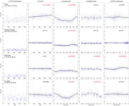
Results from fitting model (1) to a time series are the different additive functional re-5
lationships fi as shown in Fig. 2, for four exemplary locations. Here, the first row shows the model coefficients of the differentfi for a location close to Beijing (37.75◦N, 114.75◦E) representing an example with both a strong annual cycle and a strong linear trend. The second row provides an example for south Australia (22.25◦S, 125.25◦E), where the seasonal cycle is the only significant component. In the third row results for a 10
location in the North Sea, (54.25◦N, 7.75◦E) are given, with both a dependency tofann
and fwind. In the bottom row result for a location close to Milano (44.75◦N, 11.25◦E) provide an example for a significant linear trend, weekly and seasonal cycle, but a non-significant wind component (here even with a constant functionfwind).
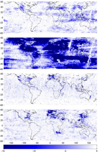
For a spatial analysis of the model terms features highlighting specific properties of 15
the differentfi, were mapped at a global scale: Fig. 3 shows p-values of the different model terms-characterizing the significance for the different components. Amplitudes of the differentfi are shown in Fig. 4. Figures 5 to 10, map individual coefficients of the weekly cycle, seasonal cycle and the wind term. In the following these maps will be studied in detail. It should be kept in mind, however, that the purpose of these maps is 20
to highlight specific features of the model terms. Patterns identified in the global map are to be checked with the actual functional form of the differentfi.
4.1 Annual cycle
ACPD
9, 9367–9398, 2009Analysing spatio-temporal patterns of the global
NO2-distribution
M. Hayn et al.
Title Page
Abstract Introduction
Conclusions References
Tables Figures
◭ ◮
◭ ◮
Back Close
Full Screen / Esc
Printer-friendly Version
Interactive Discussion sonal component is more appropriate for the description of the temporal variation of the
tropospheric NO2 VCD. The flexibility of the nonparametric model provides additional information about the annual cycle, such as the temporal distance between minimum and maximum or the number of maxima during one year.
The p-values for the annual cycle (Fig. 3) vary in space on large scales only. This 5
indicates that climatic conditions are expected to have the major impact instead of hu-man sources. In regions with strong influence of biomass burning, lightning activity or soil emissions (Jaegle et al., 2004; van der A et al., 2008), the respective emis-sions are directly connected to the seasonal variation of temperature, precipitation and convective activity.
10
In addition, the variation of the atmospheric lifetime as well as wind speed and di-rection influence the observed tropospheric NO2 patterns (this is also important for regions with mainly anthropogenic emissions). The “significant annual cycle” in the source free regions over the southern Indian Ocean is probably an artefact caused by the stratospheric correction mentioned in Sect. 2.
15
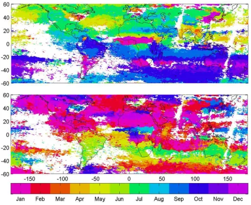
The annual component contains information on possible sources and lifetime of NO2. In Fig. 5, the month with the maximum NO2TVCD is shown. In regions with high an-thropogenic emissions the highest values are typically observed in winter time (e.g. in east Asia or the US East coast) indicating high emissions (due to heating) and high at-mospheric lifetimes. In some highly polluted regions, however, the highest values are 20
found in other months (see also Fig. 2, North Sea). This might be due to the influence of other parameters like e.g. wind speed and direction.
This indicates that transport processes should be studied separately for summer and winter. Another feature is the winter maximum in the Russian Federation along the Trans-Siberian Railway. The very low temperatures in Northern Russia might cause 25
extremely long lifetimes in those regions during winter.
ACPD
9, 9367–9398, 2009Analysing spatio-temporal patterns of the global
NO2-distribution
M. Hayn et al.
Title Page
Abstract Introduction
Conclusions References
Tables Figures
◭ ◮
◭ ◮
Back Close
Full Screen / Esc
Printer-friendly Version
Interactive Discussion al., 2008) for most locations. However, in some regions (e.g. the western USA) also
systematic differences were found, which are mainly related to the application of the non-parametric description of the annual cycle. An additional reason might be that dif-ferent periods of time are considered, during which the conditions might have changed.
4.2 Linear trend 5
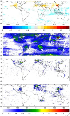
In Fig. 4, the spatial distribution of linear trends with p-values less than 0.001 for the period 1996–2001 are shown. Significant trends appear mostly in areas with dominant anthropogenic sources. We also obtain low p-values for linear trends which show al-most constant behaviour, such as in wide areas of the Indian and Pacific Ocean. It is interesting to note that these areas form the compliment to the areas with significant 10
seasonality.
Significant positive trends appear in China (up to ap-prox. 7×10¹¹[molecules] cm−2day−1=2.6×10¹⁴[molecules] cm−2year−1), in the west of USA (up to approx. 1.5×10¹⁴[molecules] cm−2year−1) and in the Mid-dle East (up to approx. 6.2×10¹³[molecules] cm−2year−1). Negative slopes 15
occur less often and with lower statistic significance. Examples are some Eu-ropean regions (approx. −1.7×10¹⁴[molecules] cm−2year−1, see also Fig. 2), the east of USA (approx. −1.19×10¹⁴[molecules] cm−2year−1) and Japan (ap-prox.−1.15×10¹⁴[molecules] cm−2year−1).
The determined linear trends are in reasonable qualitative agreement with those 20
ACPD
9, 9367–9398, 2009Analysing spatio-temporal patterns of the global
NO2-distribution
M. Hayn et al.
Title Page
Abstract Introduction
Conclusions References
Tables Figures
◭ ◮
◭ ◮
Back Close
Full Screen / Esc
Printer-friendly Version
Interactive Discussion 4.3 Weekly cycle
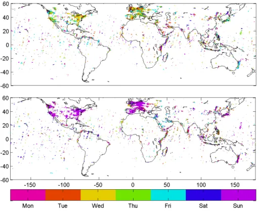
The significance of the weekly cycle changes on much smaller spatial scales than it is the case for the annual cycle (Fig. 3). In particular we notice high significances in densely settled and highly industrialized regions. A closer look confirms that many significant points in the global map coincide with big cities.
5
In Fig. 6 the weekday with minimum NO2TVCD is shown. In the USA, the minima occur mostly on Sunday, when traffic and industrial activity is reduced. The same is true for most regions in Europe and Japan. In cities of the Middle East, the minimum day is on Friday, in Israel the according to the Islamic culture. We can even point out, that the Jewish Sabbath on Saturday in Israel is detected as a significant minimum during the 10
week. No weekend effect could be detected in the big anthropogenic sources of China and South Africa. These findings agree very well with results of former publications (Beirle et al., 2003).
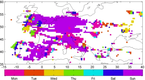
It is interesting to take a closer look on the dependence of the day of the minimum NO2 TVCD in the plume of strong anthropogenic sources with a strong weekly cycle 15
as in Europe (see Fig. 8). The original Sunday minimum in Western Europe moves eastwards with the dominating west winds. Accordingly the minimum in east Poland occurs on Monday, in the Ukraine on Tuesday, and in Western Russia on Wednesday. This gives an impression about the extent of the influence of NOx emitted (mainly) in Western Europe. We recognize that the lifetime is long enough to follow this minimum 20
in the plume during a time of four days. Here it should be noted that such long lifetime can be expected only in the winter months.
When applying this model, we obtain information about the temporal behaviour of sources, but also about the area influenced by a source that shows a characteristic temporal behaviour. Such results might be important input for model simulations of 25
ACPD
9, 9367–9398, 2009Analysing spatio-temporal patterns of the global
NO2-distribution
M. Hayn et al.
Title Page
Abstract Introduction
Conclusions References
Tables Figures
◭ ◮
◭ ◮
Back Close
Full Screen / Esc
Printer-friendly Version
Interactive Discussion obtained from the wind term in Eq. (1) discussed in the following.
4.4 Influence of wind
The wind term increased the accuracy of the model over large areas over the whole globe (Fig. 3, bottom). As expected, we find areas with a highly significant contribu-tion of the wind term close to strong continuous sources, such as the East coast of 5
the USA and east Asia, the west coast of European countries and Arabia, and in the environments of point sources like Johannesburg and Hongkong (see also Fig. 1).
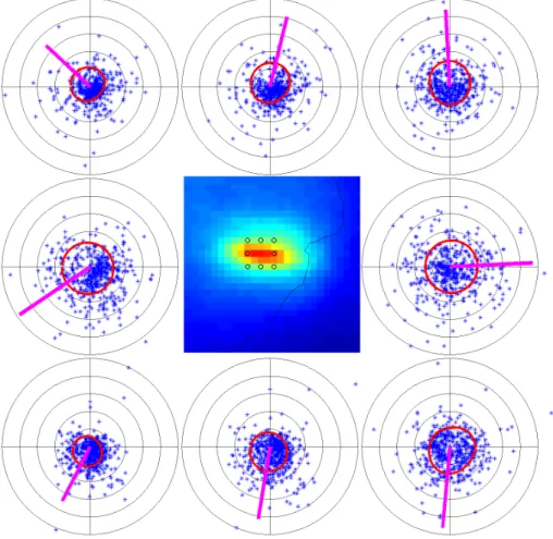
We investigate the dependence on the wind direction in more detail for several points located on a circle around the point of maximal mean NO2TVCD (Fig. 9). It is obvious that the angle corresponding to the maximum NO2 TVCD changes according to the 10
position. The highest NO2TCVDs are consistently observed from the direction of the strong emission source.
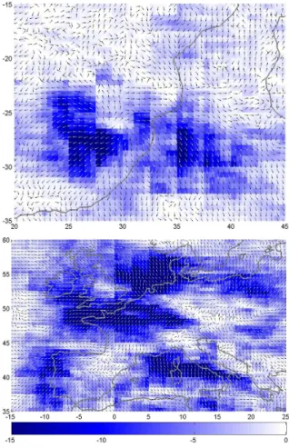
For a larger area of the region of Johannesburg, these directions are shown in Fig. 10a (black arrow), together with an indicator of the significance of the wind com-ponent (blue color). It is interesting to note that the location of the source corresponds 15
to low significance, as the wind direction is not of importance at this point. In the sur-rounding of Johannesburg the directions of the maximal wind direction form a highly ordered vector field, even for areas with a rather low significance of the wind term. Tracking the directions – the arrows in Fig. 10a – leads to large continuous “path ways” all of which leading to the Johannesburg region, and indicating those regions where 20
the central emitter is the major source for non-local NO2. In the Johannesburg region these zone of wind-related transportation extending in particular over sea, in western and eastern direction and up to more than 1000 km. Similar dependencies on the wind-related transport and characteristic emitting point sources in the center could be found for Hong-Kong, Los Angeles, Ar Riyad (Saudi Arabia), Jakarta, although not as sharp 25
as for Johannesburg.
France/South-ACPD
9, 9367–9398, 2009Analysing spatio-temporal patterns of the global
NO2-distribution
M. Hayn et al.
Title Page
Abstract Introduction
Conclusions References
Tables Figures
◭ ◮
◭ ◮
Back Close
Full Screen / Esc
Printer-friendly Version
Interactive Discussion East England which are located close to the main industrial areas of western Europe.
For the regions of the main emission sources e.g. in Benelux/Germany and in the Po valley, the wind component is not significant (compare also Fig. 2, Milano). Here the observed NO2 is dominated by local (constant) sources. It should be noted that the wind directions for maximum observed NO2TVCD do not necessarily indicate the 5
directions of the sources contributing the most to the observed NO2.
Overall, for large areas – in particular in vicinity to the major industrial areas in the Northern Hemisphere – the use of the wind component increased the prediction accu-racy significantly (Fig. 3). With the correlation between wind and observed NO2 result-ing from a local transport of the trace gas, this model extension may help to uncouple 10
the signal from transport and local generation.
Hence, a more accurate model also helps to get a clearer signal from the other effects.
5 Conclusions
We successfully applied generalized additive models (GAM) to global satellite obser-15
vations of tropospheric NO2(i.e., NO2TVCD) from 1996 to 2001. Since GAM does not require regularly sampled data (as it is the case for Fourier analysis), it can be easily applied to satellite observations, which usually contain gaps (e.g. caused by clouds). Thus, in contrast to previous studies, which are based on monthly mean values, our results are based on daily satellite observations.
20
In this study, we could detect a number of features of the temporal behaviour of the time series of the global tropospheric NO2distribution. Annual cycles could be mainly attributed to natural sources or variations of the atmospheric lifetime. Significant linear trends could be found in industrialized regions. Clear weekly cycles appeared in urban areas indicating anthropogenic sources. The location of extremes during the cycles 25
ACPD
9, 9367–9398, 2009Analysing spatio-temporal patterns of the global
NO2-distribution
M. Hayn et al.
Title Page
Abstract Introduction
Conclusions References
Tables Figures
◭ ◮
◭ ◮
Back Close
Full Screen / Esc
Printer-friendly Version
Interactive Discussion with former studies.
The non-parametric GAM also allowed to include more complex components like e.g. the wind fields. Including the wind direction from ECMWF data in the model, we could investigate transport processes of plumes of isolated point sources and polluted regions. The wind component was found to be of high importance wherever strong 5
sources border on regions free of permanent sources, like oceans. It was also possible to identify possible pathways of atmospheric pollution and to determine the extent of areas influenced by strong NO2 emission sources. Such information is important for the correct description of emission sources in atmospheric models.
Our study was limited with respect to several aspects, which should be improved in 10
future studies. The spatial resolution and coverage as well as the temporal sampling of the GOME observations is rather coarse; also the effects of changing sensitivity close to the surface and the influence of clouds on the satellite observations were addressed in a rather simplified way. In the future, increasing satellite data sets with improved spatio-temporal coverage, higher spatial resolution and improved cloud correction will 15
become available. Using such data sets will allow much more detailed studies, tak-ing into account e.g. also the wind speed, vertical wind profiles or additional quantities like temperature and precipitation. Here generalized additive models will provide ideal means for a joint, explorative analysis of observational data from multiple sources, al-lowing to access information of complex spatio-temporal pattern easily and to visualize 20
them at a global level.
Acknowledgements. We acknowledge ESA for providing the GOME-spectra. Furthermore, we want to thank ECMWF for permitting access to the ECMWF archives. Bjoern Menze acknowl-edges support by the German National Academy of Sciences Leopoldina.
References 25
ACPD
9, 9367–9398, 2009Analysing spatio-temporal patterns of the global
NO2-distribution
M. Hayn et al.
Title Page
Abstract Introduction
Conclusions References
Tables Figures
◭ ◮
◭ ◮
Back Close
Full Screen / Esc
Printer-friendly Version
Interactive Discussion Beirle, S., Platt, U., Wenig, M., and Wagner, T.: Weekly cycle of NO2by GOME measurements:
a signature of anthropogenic sources, Atmos. Chem. Phys., 3, 2225–2232, 2003, http://www.atmos-chem-phys.net/3/2225/2003/.
Beirle, S.: Estimating source strengths and lifetime of Nitrogen Oxides from satellite data, PhD thesis, Ruperto-Carola University of Heidelberg, Germany, 2004.
5
Beirle, S., Platt, U., Wenig, M., and Wagner, T.: NOx production by lightning estimated with
GOME, Adv. Space Res., 793–797, 2004.
Boersma, K. F., Eskes, H. J., and Brinksma, E. J.: Error analysis for tropospheric NO2 retrieval from space, J. Geophys. Res., 109, D04311, doi:10.1029/2003JD003962, 2004.
Bovensmann, H., Burrows, J. P., Buchwitz, M. et al.: SCIAMACHY: Mission Objectives and 10
Measurement Modes, J. Atmos. Sci., 56(2), 127–150, 1999.
Brillinger, D.: An application of statistics to meteorology: estimation of motion, in:Festschrift for Lucien Le Cam, edited by: Pollard, D. and Yang, G., Springer, New York, 1994.
Burrows, J. P., Weber, M., Buchwitz, M., et al.: The Global Ozone Monitoring Experiment (GOME): Mission concept and first results, J. Atmos. Sci., 56, 151–175, 1999.
15
Craven, P. and Wahba, G.: Smoothing noisy data with spline functions, Numer. Math., 31, 377–403, 1979.
Dominici, F., McDermott, A., S. L. Zeger, et al.: On the Use of Generalized Additive Models in Time-Series Studies of Air Pollution and Health, Am. J. Epidemiol., 156(3), 193–203, 2002. Elsayed, N. M.: Toxicity of nitrogen dioxide: an introduction, Toxicology, 89(3), 161–74, 1994. 20
ESA: Global Ozone Monitoring Experiment (GOME), Users Manual, ESA Publications Devi-sion, SP-1182, edited by: Bednarz, F., ISBN: 92-9092-327, 1995.
Grzegorski, M., Wenig, M., Platt, U., Stammes, P., Fournier, N., and Wagner, T.: The Heidelberg iterative cloud retrieval utilities (HICRU) and its application to GOME data, Atmos. Chem. Phys., 6, 4461–4476, 2006, http://www.atmos-chem-phys.net/6/4461/2006/.
25
Hastie, T. J. and Tibshirani, R. J.: Generalized Additive Models, Statistical Science, 1(3), 297– 318, 1986.
Hastie, T. J. and Tibshirani, R. J.: Generalized Additive Models, Chapman & Hall/CRC, 1990. Jacob, D. J.: Introduction to Atmospheric Chemistry, Princeton University Press, 1999.
Jaegl ´e, L., Martin, R. V., Chance, K., et al.: Satellite mapping of rain-induced nitric oxide emis-30
sions from soils, J. Geophys. Res., 109, D21310, doi:10.1029/2004JD004787, 2004. K ˚allberg, P., Simmons, A., Uppala, S., and Fuentes, M.: ECMWF: The 40 Archive,
ACPD
9, 9367–9398, 2009Analysing spatio-temporal patterns of the global
NO2-distribution
M. Hayn et al.
Title Page
Abstract Introduction
Conclusions References
Tables Figures
◭ ◮
◭ ◮
Back Close
Full Screen / Esc
Printer-friendly Version
Interactive Discussion Kim, J. and Hong, J.: A GAM for Daily Ozone Concentration in Seoul, Key Eng. Mat., 277–279,
497–502, 2005.
Leue, C., Wenig, M., Wagner, T., Klimm, O., Platt, U., and J ¨ahne, B.: Quantitative analysis of NOx emissions from GOME satellite image sequences, J. Geophys. Res., 106(D6), 5493–
5505, 2001. 5
Martin, R. V., Chance, K., Jacob, D. J., et al.: An improved retrieval of tropospheric nitrogen dioxide from GOME, J. Geophys. Res., 107(D20), 4437, doi:10.1029/2001JD001027, 2002. McCullagh, P. and Nelder, J. A.: Generalized Linear Models, London: Chapman and Hall,
1989.
Olivier et al.: Global air emission inventories for anthropogenic sources of NOx, NH3 and N2O
10
in 1990, Environ. Pollut., 102, 135–148, 1990.
Platt, U.: Differential optical absorption spectroscopy (DOAS), In: Sigrist, M., editor, Air Moni-toring by Spectrometric Techniques, 27–84, John Wiley, New York, 1994.
Richter, A. and Burrows, J. P.: Tropospheric NO2 from GOME Measurements, Adv. Space Res., 29(11), 1673–1683, 2002.
15
Richter, A., Burrows, J. P., N ¨uß, H., Granier, C., and Niemeier, U.: Increase in tropospheric nitrogen dioxide over China observed from space, Nature, 437(7055), 129–132, 2005. Seinfeld, J. H. and Pandis, S. N.: Atmospheric Chemistry and Physics, John Wiley and Sons,
1997.
Smith, R. L., Davis, J. M., and Speckman, P.: Human health effects of environmental pollution 20
in the atmosphere, In: Barnett V, Stein A, Turkman F, eds. Statistics in the environment 4: statistical aspects of health and the environment, 91–115, Chichester, United Kingdom: John Wiley & Sons Ltd, citeseer.ist.psu.edu/rl99human.html, 1999.
Solomon, S., Schmeltekopf, A. L., and Sanders, R. W.: On the interpretation of zenith sky absorption measurements, J. Geophys. Res., 92, 8311–8319, 1987.
25
Stige, L. C., Stave, J., Chan, K.-S., Ciannelli, L., Pettorelli, N., Glantz, M., Herren, H. R., and Stenseth, N. C.: The effect of climate variation on agro-pastoral production in Africa, Proceedings of the National Academy of Sciences, PNAS, 103(9), 2006.
Stohl, A., Huntrieser, H., Richter, A., Beirle, S., Cooper, O. R., Eckhardt, S., Forster, C., James, P., Spichtinger, N., Wenig, M., Wagner, T., Burrows, J. P., and Platt, U.: Rapid intercontinental 30
air pollution transport associated with a meteorological bomb, Atmos. Chem. Phys., 3, 969– 985, 2003, http://www.atmos-chem-phys.net/3/969/2003/.
ACPD
9, 9367–9398, 2009Analysing spatio-temporal patterns of the global
NO2-distribution
M. Hayn et al.
Title Page
Abstract Introduction
Conclusions References
Tables Figures
◭ ◮
◭ ◮
Back Close
Full Screen / Esc
Printer-friendly Version
Interactive Discussion Springer-Lehrbuch, 2008.
Uno, I., Ohara, T., and Wakamatsu, S.: Analysis of wintertime NO2 pollution in the Tokyo
Metropolitan area, Atmos. Environ., 30(5), 703–713(11), 1996.
van der A, R. J., Peters, D. H. M. U.,, Eskes, Boersma, K. F., Van Roozendael, M., De Smedt, I., and Kelder, H. M.: Detection of the trend and seasonal variation in tropospheric NO2over
5
China, J. Geophys. Res., 111, D12317, doi:10.1029/2005JD006594 2006.
van der A, R. J., Eskes, H. J., Boersma, K. F., van Noije, T. P. C., Van Roozendael, M., De Smedt, I., Peters, D. H. M. U., Kuenen, J. J. P., and Meijer, E. W.: Identification of NO2
sources and their trends from space using seasonal variability analyses, J. Geophys. Res., 113, doi:10.1029/2007JD009021, 2008.
10
Velders, G. J. M., Granier, C., Portmann, R. W., Pfeilsticker, K., Wenig, M., Wagner, T., Platt, U., Richter, A., and Burrows, J. P.: Global tropospheric NO2 column distributions:
Com-paring three-dimensional model calculations with GOME measurements, J. Geophys. Res., 106(D12), 12643–12660, 2001.
Wagner, T., Beirle, S., Deutschmann, T., Eigemeier, E., Frankenberg, C., Grzegorski, M., Liu, 15
C., Marbach, T., Platt, U., and Penning de Vries, M.: Monitoring of atmospheric trace gases, clouds, aerosols and surface properties from UV/vis/NIR satellite instruments, J. Opt. A: Pure Appl. Opt., 10, 104019, doi:10.1088/1464-4258/10/10/104019, 2008.
Wakamatsu, S., Uno, I., and Ohara, T.: Springtime Photochemical Air Pollution in Osaka: Field Observation, J. Appl. Meteorol., 37, 1100–1106, 1998.
20
Wenig, M., Spichtinger, N., Stohl, A., Held, G., Beirle, S., Wagner, T., J ¨ahne, B., and Platt, U.: Intercontinental transport of nitrogen oxide pollution plumes, Atmos. Chem. Phys., 3, 387–393, 2003, http://www.atmos-chem-phys.net/3/387/2003/.
Wood, S. N.: Generalized Additive Models: An Introduction with R, Chapman & Hall/CRC, Taylor & Francis Group, 2006.
25
ACPD
9, 9367–9398, 2009Analysing spatio-temporal patterns of the global
NO2-distribution
M. Hayn et al.
Title Page
Abstract Introduction
Conclusions References
Tables Figures
◭ ◮
◭ ◮
Back Close
Full Screen / Esc
Printer-friendly Version
Interactive Discussion Fig. 1. Left: Mean tropospheric vertical column density (TVCD) of NO2 (10
15
ACPD
9, 9367–9398, 2009Analysing spatio-temporal patterns of the global
NO2-distribution
M. Hayn et al.
Title Page
Abstract Introduction
Conclusions References
Tables Figures
◭ ◮
◭ ◮
Back Close
Full Screen / Esc
Printer-friendly Version
Interactive Discussion Fig. 2. Examples of the GAM components for China, Central Australia, the North Sea, and
ACPD
9, 9367–9398, 2009Analysing spatio-temporal patterns of the global
NO2-distribution
M. Hayn et al.
Title Page
Abstract Introduction
Conclusions References
Tables Figures
◭ ◮
◭ ◮
Back Close
Full Screen / Esc
Printer-friendly Version
Interactive Discussion Fig. 3. The significance (log10 of the p-value) of the different GAM terms, i.e. trend, annual
ACPD
9, 9367–9398, 2009Analysing spatio-temporal patterns of the global
NO2-distribution
M. Hayn et al.
Title Page
Abstract Introduction
Conclusions References
Tables Figures
◭ ◮
◭ ◮
Back Close
Full Screen / Esc
Printer-friendly Version
Interactive Discussion Fig. 4.The strength of the different GAM terms.(a)Absolute trend in 1014molec/cm2per year.
ACPD
9, 9367–9398, 2009Analysing spatio-temporal patterns of the global
NO2-distribution
M. Hayn et al.
Title Page
Abstract Introduction
Conclusions References
Tables Figures
◭ ◮
◭ ◮
Back Close
Full Screen / Esc
Printer-friendly Version
ACPD
9, 9367–9398, 2009Analysing spatio-temporal patterns of the global
NO2-distribution
M. Hayn et al.
Title Page
Abstract Introduction
Conclusions References
Tables Figures
◭ ◮
◭ ◮
Back Close
Full Screen / Esc
Printer-friendly Version
ACPD
9, 9367–9398, 2009Analysing spatio-temporal patterns of the global
NO2-distribution
M. Hayn et al.
Title Page
Abstract Introduction
Conclusions References
Tables Figures
◭ ◮
◭ ◮
Back Close
Full Screen / Esc
Printer-friendly Version
ACPD
9, 9367–9398, 2009Analysing spatio-temporal patterns of the global
NO2-distribution
M. Hayn et al.
Title Page
Abstract Introduction
Conclusions References
Tables Figures
◭ ◮
◭ ◮
Back Close
Full Screen / Esc
Printer-friendly Version
Interactive Discussion Fig. 8. Day of week with minimum TVCD (see Fig. 6b) for Europe. Over most regions, the
minimum occurs on Sunday. In eastern Europe the minimum is shifted to the beginning of the week indicating the transport of the temporal emission patterns of the strong western NOx
ACPD
9, 9367–9398, 2009Analysing spatio-temporal patterns of the global
NO2-distribution
M. Hayn et al.
Title Page
Abstract Introduction
Conclusions References
Tables Figures
◭ ◮
◭ ◮
Back Close
Full Screen / Esc
Printer-friendly Version
Interactive Discussion Fig. 9.The dependencies of the NO2TVCD (red circle indicates the fitted spline) on the wind
direction for 8 points around Johannesburg (see image in the center). The wind direction of maximum NO2TVCD (pink pointer indicate the direction of the air flux) changes accordingly to
ACPD
9, 9367–9398, 2009Analysing spatio-temporal patterns of the global
NO2-distribution
M. Hayn et al.
Title Page
Abstract Introduction
Conclusions References
Tables Figures
◭ ◮
◭ ◮
Back Close
Full Screen / Esc
Printer-friendly Version
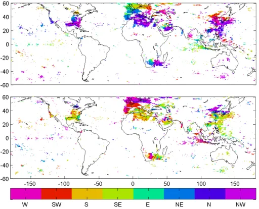
Interactive Discussion Fig. 10. Wind direction of maximum TVCD as quiver-plot (compare Fig. 7a) for the region(a)