Geosci. Model Dev., 8, 2435–2445, 2015 www.geosci-model-dev.net/8/2435/2015/ doi:10.5194/gmd-8-2435-2015
© Author(s) 2015. CC Attribution 3.0 License.
Revision of the convective transport module CVTRANS 2.4 in the
EMAC atmospheric chemistry–climate model
H. G. Ouwersloot1, A. Pozzer1, B. Steil1, H. Tost2, and J. Lelieveld1
1Atmospheric Chemistry Department, Max Planck Institute for Chemistry, Mainz, Germany 2Institute for Atmospheric Physics, University of Mainz, Mainz, Germany
Correspondence to:H. G. Ouwersloot (huug.ouwersloot@mpic.de)
Received: 9 March 2015 – Published in Geosci. Model Dev. Discuss.: 8 April 2015 Revised: 26 June 2015 – Accepted: 16 July 2015 – Published: 5 August 2015
Abstract. The convective transport module, CVTRANS, of the ECHAM/MESSy Atmospheric Chemistry (EMAC) model has been revised to better represent the physical flows and incorporate recent findings on the properties of the con-vective plumes. The modifications involve (i) applying inter-mediate time stepping based on a settable criterion, (ii) us-ing an analytic expression to account for the intra-time-step mixing ratio evolution below cloud base, and (iii) implement-ing a novel expression for the miximplement-ing ratios of atmospheric compounds at the base of an updraft. Even when averaged over a year, the predicted mixing ratios of atmospheric com-pounds are affected considerably by the intermediate time stepping. For example, for an exponentially decaying atmo-spheric tracer with a lifetime of 1 day, the zonal averages can locally differ by more than a factor of 6 and the induced root mean square deviation from the original code is, weighted by the air mass, higher than 40 % of the average mixing ratio. The other modifications result in smaller differences. How-ever, since they do not require additional computational time, their application is also recommended.
1 Introduction
A key process in global modeling of atmospheric chemistry and climate is the vertical exchange of air (Lelieveld and Crutzen, 1994). Convective vertical motions redistribute en-ergy, moisture and reactive trace species between different vertical layers within the troposphere. For clear sky condi-tions, this transport between e.g., Earth’s surface and the top of the troposphere acts on timescales on the order of weeks. However, moist convective transport associated with
cumuli-form clouds reduces it to time periods of hours (Lawrence and Rasch, 2005; Tost et al., 2010). Especially short-lived atmospheric compounds are strongly affected. Although im-portant, the convective clouds cannot be explicitly resolved in general circulation models and need to be parameterized (e.g., Arakawa, 2004; Kim et al., 2012). Useful tools to de-rive and check these parameterizations are large-eddy sim-ulation (LES) models that operate in smaller domains with a higher resolution (e.g., Bechtold et al., 1995; Siebesma and Cuijpers, 1995; Ouwersloot et al., 2013).
layer can affect the properties of the air that enters the con-vective plumes from below. The improvement to the convec-tive transport parameterization proposed in this study is ap-plied here as well. In addition to assessing the effects of the aforementioned revisions, we evaluate the impact of a dif-ferent convective cloud cover representation on convective transport.
In Sect. 2 we describe the model and applied modifica-tions. The setup to study the induced changes is presented in Sect. 3. These differences are then quantified and discussed in Sect. 4.
2 Model
2.1 Original representation of convection
In this study we apply and improve version 2.50 of the MESSy (Modular Earth Submodel System) framework (Jöckel et al., 2005, 2010), which is an interface structure that connects a base model to various submodels. Although our modifications are applicable to different base models as well, we validate the results using the EMAC model, first described by Jöckel et al. (2006). This system combines MESSy with version 5.3.02 of the European Centre Ham-burg general circulation model (ECHAM5; Roeckner et al., 2006).
The moist convective transport for tracers other than wa-ter is calculated by the CVTRANS submodel (Tost et al., 2010), which represents the bulk formulation for convective plumes described by Lawrence and Rasch (2005). A single plume, also referred to as “leaky pipe”, is considered for the updrafts and downdrafts separately. These plumes can later-ally entrain and detrain at every level, resulting in a vertical mass flux that varies with height. The fluxes themselves, in kg m−2s−1, are not calculated in CVTRANS, but are
gath-ered from the CONVECT submodel (Tost et al., 2006). In the algorithm, the properties of the air that detrains from the plumes are determined according to1
Cup, det.k =
Dupk −fdEupk
Cupk+1+fdEupk Cenv.k
Dk up
, (1)
Cdown, det.k =Ckdown, (2)
where k is the height index, decreasing with altitude. The subscripts up, down and env. indicate properties of respec-tively the updraft, the downdraft and the ambient air in the cloud environment. If additionally the subscript det. is used, the variable represents the property of air that is detrained from the plume in that grid cell. C is the mixing ratio (in mol mol−1), andD andE are respectively the rates of de-trainment from and ende-trainment into the convective plume
1Note that (only) the mass fluxes and mixing ratios in the up- and
downdraft plumes are specified at the top interface of the indexed grid cell.
(in kg m−2s−1). Part of the air that is entrained in the
up-draft is detrained again in the same grid cell (Lawrence and Rasch, 2005). The fraction of entrained air in a layer that is detrained again in the same layer is denoted byfd.
Al-though this fraction is dependent on multiple factors, includ-ing grid resolution, it is generally set to a value of 0.5. If necessary,fd is adapted to ensure that the detrained mass
flux that originates from the entrained air,fdEupk , never
ex-ceeds the total detrained mass flux,Dupk , and that fdEupk is
high enough so that the total amount of detrained air from the plume,Dupk , does not exceed Fupk+1+fdEupk . Fk is the
mass flux (in kg m−2s−1) at the top interface of grid levelk. The mixing ratios in the plumes, which are also needed for Eqs. (1) and (2), are instantaneously calculated as
Cupk =F k+1
up Cupk+1−DkupCup, det.k +Eupk Cenv.k Fk
up
, (3)
Cdownk+1 =F k downC
k down−D
k downC
k
down, det.+E k downCenv.k
Fdownk+1 . (4)
The mixing ratio in the updraft plume is initialized at the low-est level where the mass flux exceeds 0, indicated by index
kb. In the original CVTRANS 2.3 code Ckb
up=C kb
env.. (5)
The temporal evolution of the mixing ratios in the grid cells parts that are affected by the plumes is expressed by
Cenv.k (t+1t )=M k orig
Mk C
k env.(t )+
1t
Mk (6)
×
Fupk −Fdownk
Cenv.k−1+DkupCup, det.k +Ddownk Cdown, det.k
,
where1tis the time step andMorigis the mass per unit area
of air (in kg m−2) whose mixing ratio is not altered due to the plumes in one time step. This is calculated as
Morigk =Mk−1t
Fupk −Fdownk
+Dkup+Dkdown
. (7)
Mwithout subscript is the total mass per unit area of air in which plumes occur in the grid cell, calculated as the total air mass per unit area in that grid cell times a certain cover. This cover can be selected as 1 or as the more representative con-vective cloud cover, calculated in the CONVECT module. 2.2 Modifications to CVTRANS 2.4
2.2.1 Intermediate time steps
flow is no longer properly represented. To remedy these is-sues we introduce intermediate time stepping in CVTRANS 2.4, where we divide the global time step in sub-time steps with length1tsub. The amount of sub-time steps per global
time step is determined per vertical column to ensure that at every level,k,
Fupk1tsub< fmaxfracmin(Mk, Mk−1). (8)
Here,fmaxfracis an a priori chosen fraction ofM that is
al-lowed to leave the grid cell through the upward plume per sub-time step. This fraction is set in the updated CVTRANS namelist. For every horizontal location the convective trans-port in the column is calculated independently in CVTRANS 2.4 using the locally required amount of sub-steps.
2.2.2 Analytic expression at cloud base
Near the convective cloud base, we can account for recircu-lation effects within a single time step in a computationally less inexpensive manner by applying an analytic solution for the sub-cloud mixing ratio evolution. At cloud base levelkb, Ckb
envevolves in time according to ∂
∂tM
kbCkb
env= −FupkbCkenvb
| {z }
upward plume
+ Fkb
upCenvkb−1
| {z }
compensating subsidence
, (9)
since air leaves the grid cell with properties of the environ-mental air and is replenished by compensating subsidence with properties of the environmental air in the overlying grid cell. During the time step the mass and mass fluxes do not change, resulting in
hCkb
envi =C kb−1
env,0+
Ckb
env,0−C kb−1
env,0
1−e−ffrac
ffrac
, (10)
ffrac= Fkb
up1tsub
Mkb , (11)
whereh iindicates a temporal average over the sub-time step and subscript 0 refers to the value at the start of the sub-time step. UsinghCkb
enviinstead ofCenv.kb in Eq. (5) does not yield
substantially different results if F
kb
up1tsub
Mkb ≪1. Otherwise, this revised representation accounts for the major influence of the updraft plume on the sub-plume mixing ratio evolution within the time step and for the resulting reduced impact of vertical mixing ratio gradients around the plume base. 2.2.3 Altered concentrations at updraft base
As a third modification, we include a recently published pa-rameterization for the vertical transport of chemical reactants at the convective cloud base (Ouwersloot et al., 2013). Re-lated to induced large-scale circulations in the convective boundary layer below the convective plumes, it was found that the mixing ratios of atmospheric chemical species at the
base of the updraft plume,Ckb
up, differ even more fromCenvkb−1
thanCkb
env. ConsideringCenvkb to be representative for the
mix-ing ratio in the sub-cloud layer, their Eq. (13) is applied by replacing our Eq. (5) by
Ckb
up=Cenvkb +(ftrans−1)
Ckb
env−Cenvkb−1
, (12)
whereftrans is a namelist setting with a standard value of
1.23 (Ouwersloot et al., 2013). When both this parameteri-zation and the analytic solution below the cloud base are ap-plied, Eq. (5) is again replaced by Eq. (10), while Eq. (11) is updated to
ffrac=
ftransFupkb1tsub
Mkb . (13)
These updated mixing ratios are only applied if the updraft plume is affected by convective boundary-layer dynamics. This is considered to be the case if the bottom of the plume is located below the boundary-layer height that is diagnosed by the TROPOP module or below a height limit that can be set in the CVTRANS namelist. In this study it is kept to the standard setting of 2500 m.
3 Simulation setup
We performed numerical simulations with EMAC to quan-tify the impact of the various code modifications. In these simulations, the MESSy submodels that are listed in Table 1 have been enabled. Unless specified differently, standard set-tings are used. For illustration purposes, the convective trans-port is tested for the standard convection parameterization in EMAC, which is based on Tiedtke (1989) and Nordeng (1994). The simulations are all performed at the T63 horizon-tal resolution (192×96 grid) with 31 vertical hybrid pressure levels and a time step of 12 min. The simulation period spans the years 2000 and 2001, of which the former year is consid-ered spinup time. The initial state is prescribed by ECMWF (European Centre for Medium-Range Weather Forecasts) op-erational analysis data. To check the undisturbed effects of the applied modifications, no nudging is applied to meteoro-logical data during the simulation.
Table 1.Optional MESSy submodels that are enabled for the numerical experiments.
Submodel Executed process Reference
CLOUD Original ECHAM5 cloud formation Roeckner et al. (2006) CONVECT Convection Tost et al. (2006) CVTRANS Convective tracer transport Tost et al. (2010) and text OFFEMIS Prescribed emissions of trace gases Kerkweg et al. (2006) PTRAC Prognostic tracers Jöckel et al. (2008) TNUDGE Pseudo-emissions of tracers Kerkweg et al. (2006) TREXP Exponentially decaying tracers Jöckel et al. (2010) TROPOP Tropopause and boundary-layer diagnostics Jöckel et al. (2006) VISO Diagnostics at isosurfaces Jöckel et al. (2010)
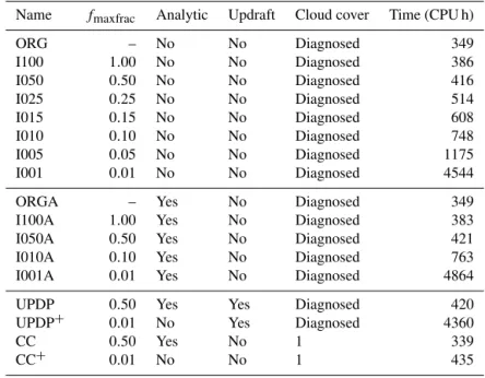
Table 2.Description of the different numerical experiments. Listed are the differences in settings between the simulations and required computational time (in CPU hours). Iffmaxfracis set to –, intermediate time steps are not enabled. The columns Analytic and Updraft denote
respectively whether the analytic expression and the updated concentrations at the updraft base are applied. The applied cloud cover is either diagnosed in the CONVECT module or set to 1.
Name fmaxfrac Analytic Updraft Cloud cover Time (CPU h)
ORG – No No Diagnosed 349 I100 1.00 No No Diagnosed 386 I050 0.50 No No Diagnosed 416 I025 0.25 No No Diagnosed 514 I015 0.15 No No Diagnosed 608 I010 0.10 No No Diagnosed 748 I005 0.05 No No Diagnosed 1175 I001 0.01 No No Diagnosed 4544 ORGA – Yes No Diagnosed 349 I100A 1.00 Yes No Diagnosed 383 I050A 0.50 Yes No Diagnosed 421 I010A 0.10 Yes No Diagnosed 763 I001A 0.01 Yes No Diagnosed 4864 UPDP 0.50 Yes Yes Diagnosed 420 UPDP+ 0.01 No Yes Diagnosed 4360
CC 0.50 Yes No 1 339
CC+ 0.01 No No 1 435
Multiple numerical experiments have been performed. Ex-periments whose name start with “ORG” do not use the in-termediate time stepping, but if an experiment name starts with an “I”, it does employ the intermediate time stepping and it is followed by a three-digit number that is equal to 100×fmaxfrac. The most precise experiment, I001, thus sets fmaxfracto 0.01. Note that in our analyses,I001is considered
to represent convective tracer transport best and is used as the reference simulation to quantify deviations. If the numerical experiment is followed by an “A”, the analytic expression for the temporal evolution of mixing ratios below the convective cloud base is applied as well. In general, the adapted convec-tive transport near cloud base is not applied and we use the convective cloud cover as calculated in CONVECT to deter-mine the fractions of the grid cells that are affected by the updraft and downdraft plumes. However, numerical
experi-ments UPDP and CC, both based on numerical experiment I050A, are exceptions to this. In UPDP the adapted convec-tive transport parameterization at the updraft plume base is enabled. In CC the convective transport is calculated using a convective cloud cover of 1, representing the extreme case where convective plumes span entire grid cells. Note that the resulting mass transport per affected unit area is weaker and therefore applying intermediate time steps has less impact. To complete the quantification of differences, additional nu-merical experiments UPDP+and CC+are conducted, which
are similar to UPDP and CC but based on experiment I001 instead of I050A. An overview of the different numerical ex-periments is presented in Table 2.
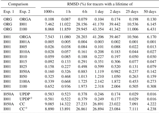
re-Table 3. Weighted root mean square deviations between two numerical experiments. Results, expressed as percentages of the respective air-mass-weighted mixing ratios, are listed for the seven tracers.
Comparison RMSD (%) for tracers with a lifetime of
Exp. 1 Exp. 2 1000 s 1 h 6 h 1 day 2 days 25 days 50 days ORG ORGA 0.108 0.087 0.079 0.104 0.174 0.198 0.130 ORG I001 7.462 11.022 28.156 41.170 39.442 10.536 6.145 ORG I100 8.068 11.859 29.945 43.354 41.342 11.006 6.431 I001 ORGA 7.543 11.080 28.203 41.206 39.467 10.566 6.170 I001 I001A 0.005 0.005 0.004 0.003 0.002 0.001 0.001 I001 I005 0.026 0.038 0.084 0.101 0.088 0.022 0.013 I001 I010A 0.028 0.057 0.161 0.208 0.183 0.044 0.027 I001 I010 0.059 0.085 0.188 0.227 0.197 0.050 0.030 I001 I015 0.092 0.133 0.291 0.351 0.306 0.077 0.047 I001 I025 0.158 0.227 0.498 0.599 0.520 0.131 0.079 I001 I050A 0.160 0.326 0.883 1.119 0.982 0.237 0.142 I001 I050 0.325 0.468 1.013 1.210 1.050 0.263 0.159 I001 I100A 0.339 0.668 1.725 2.142 1.872 0.453 0.273 I001 I100 0.652 0.936 1.973 2.318 2.004 0.505 0.308 I050A UPDP 0.583 0.523 0.378 0.246 0.174 0.029 0.016 I001 UPDP+ 0.581 0.522 0.379 0.249 0.177 0.029 0.016 I050A CC 9.085 14.322 27.233 26.891 23.022 7.091 4.222 I001 CC+ 8.890 13.891 26.861 26.894 23.084 7.111 4.238
lated to the different convective transport representations. For quantification, the root mean square deviation (RMSD) over the numerical grid is used, weighted by the air mass,M, in each grid cell. For two different simulations, denoted by in-dicators A and B, the RMSD of a mixing ratio,c, is defined as
RMSDA,B(c)= v u u t
P
iMi cA,i−cB,i 2
P iMi
, (14)
where indicatori iterates over the individual grid cells and an overbar denotes a temporal average over 2001. To put into perspective, the RMSD is always expressed as a percentage of the air-mass-weighted mixing ratio, Pi(Mici)/PiMi.
Note that the air-mass-weighted mixing ratio is the same for all numerical experiments since we evaluate chemically inert species with constant emissions.
4 Results
In Sect. 4.1 the effect of intermediate time steps on the at-mospheric compounds is shown. The effect of using the an-alytic expression, for the temporal mean mixing ratio during a time step below the updraft plume, is discussed in Sect. 4.2. Subsequently, the optimal settings for intermediate time steps and the analytic expression are determined in Sect. 4.3 for the current numerical setup. The changes induced by considering the updated parameterization for mixing ratios at the updraft
plume base and a different convective cloud cover are treated in Sects. 4.4 and 4.5, respectively.
The weighted root mean square deviations between differ-ent numerical experimdiffer-ents are listed in Table 3.
4.1 Intermediate time steps
As can be seen from Table 3, the strongest deviations are found for a lifetime of 1 or 2 days. This is related to the timescale of convective transport being on the same order of magnitude. Atmospheric compounds with longer lifetimes are generally well mixed with height and their distribution is therefore less affected by convective transport. Shorter-lived species are mainly concentrated near the sources at Earth’s surface, resulting in low mixing ratios and, consequently, low absolute deviations where convective transport is active. However, even for short (τ =1000 s) or long (τ=50 days) lifetimes, the root mean square deviations of the 2001 av-eraged mixing ratio are over 5 % of the respective weighted mean mixing ratios.
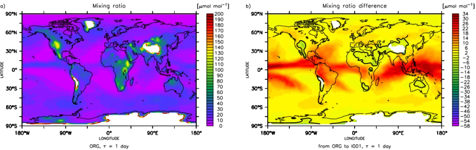
Figure 1.Horizontal distribution of the decaying scalar with a lifetime of 1 day, averaged over 2001 at 700 hPa. Shown are(a)the distribution for the ORG numerical experiment and(b)the mixing ratio difference for I001 compared to ORG.
compared to the atmospheric boundary layer, except for loca-tions where convective transport is active. From Fig. 1a it can be seen that indeed relatively high mixing ratios are found in regions that are either characterized by a high elevation, thus evaluating boundary-layer air, or by more active convection, such as the intertropical convergence zone, the South Pacific convergence zone and the westerly storm tracks.
In the ORG numerical experiment, convective transport is capped when the upward mass flux transports more air in one time step than is present in the underlying grid cell. This nonphysical capping of the flow can be removed when in-termediate time steps are enabled. As shown in Fig. 1b, this results in enhanced vertical transport and thus higher free tro-pospheric mixing ratios, particularly in the areas with strong convection. Supporting images are presented in Fig. 1 of the Supplement. In the boundary layer, as illustrated by the areas with high elevation, the mixing ratios become slightly lower due to the enhanced vertical transport. The increase in mix-ing ratios in the free troposphere are of the same order as the mixing ratios in the ORG numerical experiment and the fi-nal mixing ratios in I001 can be up to a factor of 5 higher (not shown). This high factor is mainly due to the low mix-ing ratios in ORG at those locations, which yields large rel-ative differences for small absolute mixing ratio differences. Therefore, the air-mass-weighted root mean square deviation of the 2001 averaged mixing ratios is used for the quantifica-tion, which is equal to 43 % of the air-mass-weighted mixing ratio for the tracer with a lifetime of 1 day.
The substantial change in the representation of convec-tive transport with intermediate time steps is also clear from Fig. 2, with changes over 500 % in the yearly and zonally averaged mixing ratios compared to the ORG numerical ex-periment. Although these high, relative differences typically occur in regions with relatively low mixing ratios, they can be compared to similar figures for the effects of different con-vection parameterizations (e.g., Fig. 2 in Tost et al., 2010) and of using an ensemble plume model instead of a bulk
plume model (e.g., Fig. 4 in Lawrence and Rasch, 2005). Even though mixing ratios were averaged over shorter peri-ods in those studies, much lower relative changes were found with maximum differences between 20 and 100 %. That the consequential variations in representing convective transport applied by Lawrence and Rasch (2005) and Tost et al. (2010) yield smaller differences in the distributions of trace species emphasizes the importance of applying the intermediate time steps.
Note from Table 3 that coarser intermediate time steps, e.g., I100, yield similar differences, compared to ORG as I001, and that the deviations between I001 and I100 are more than 10 times smaller. This shows that the strongest effect re-sults from the convective transport by the updraft plume no longer being capped, since in I100 entire grid cells can still be depleted of air in individual sub-time steps. Since within each intermediate time step I100 does not account for the re-circulation of air and the mass of the entire grid cell can be removed, the effectiveness of convective transport is actually overestimated, while it was underestimated in ORG. This is why the RMSD values between I100 and ORG are slightly higher than those between I001 and ORG. To better account for this recirculation, lower values forfmaxfraccan be chosen
and the analytic expression for the temporal mean mixing ra-tio below the convective cloud base can be employed.
4.2 Analytic expression
Figure 2.Decaying scalar with a lifetime of 1 day, averaged zonally and over 2001. Shown are(a)the distribution for the ORG numerical experiment and(b)the relative mixing ratio difference for I001 compared to ORG.
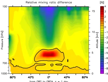
fluxes. As a result, it will no longer occur that the entire air mass in the grid cell below the plume base is replaced by environmental air from the grid cell above the plume base.
Since part of the air at the updraft plume base now orig-inates from the environment above cloud base, the effect of vertical mixing by convective transport is reduced. This re-sults in stronger vertical gradients with higher mixing ratios near the surface and higher mixing ratios in the upper tro-posphere, as confirmed in Fig. 3. Because vertical transport is underestimated in ORG, due to the capping of the mass fluxes of the updraft plumes, the RMSD between ORGA and I001 is actually higher than between ORG and I001. How-ever, for all numerical experiments with intermediate time stepping, where mass fluxes are not capped, the RMSD com-pared to I001 decreases when the analytic expression is em-ployed. This effect is especially influential for shorter lived species, roughly halving the RMSD compared to the refer-ence case forτ =1000 s.
As most clearly illustrated by the RMSD between ORG and ORGA in Table 3, the analytic expression increases in significance when the lifetime of the tracer is shorter. We hypothesize that this is related to the vertical distribution of the exponentially decaying tracers. For shorter lifetimes, a greater part of these tracers is located in the lower tro-posphere, where the effect of the represented recirculation around the cloud base is strongest.
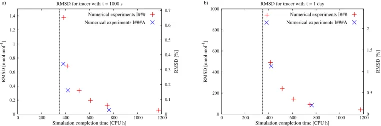
4.3 Performance
While the dynamics are best represented by using intermedi-ate time stepping with a lowfmaxfracin combination with the
analytic expression of Eq. (10), these settings can be com-putationally expensive. Therefore, an optimal setting should be chosen that limits the amount of required computational time, but results in low RMSD values compared to the ref-erence simulation, I001. For illustration, these values are
Figure 3.Relative difference in zonally and 2001 averaged mixing ratios for ORGA compared to ORG. Results are shown for the tracer with a lifetime of 1 day.
shown as a function of computational time in Fig. 4 for the tracers with lifetimes of 1000 s and 1 day. For this we take the computational time that each respective numerical exper-iment needed to finish the 2 year simulation with the settings listed in Sect. 3.
The RMSD is roughly proportional to the value offmaxfrac,
while the extra required computational time with respect to ORG scales inversely to fmaxfrac. In this setup we select fmaxfrac=0.50 as most desirable for further analyses, since
0 0.2 0.4 0.6 0.8 1 1.2 1.4
0 200 400 600 800 1000 1200 0 0.1 0.2 0.3 0.4 0.5 0.6 0.7
RMSD [nmol mol
-1]
RMSD [%]
Simulation completion time [CPU h] RMSD for tracer with τ = 1000 s a)
Numerical experiments I### Numerical experiments I###A
0 200 400 600 800 1000
0 200 400 600 800 1000 1200 0 0.5 1 1.5 2
RMSD [nmol mol
-1]
RMSD [%]
Simulation completion time [CPU h] RMSD for tracer with τ = 1 day b)
Numerical experiments I### Numerical experiments I###A
Figure 4. Root mean square deviations of the 2001 averaged mixing ratios compared to reference case I001 for decaying scalars with a lifetime of(a)1000 s and(b)1 day. On the vertical axes, the RMSD is expressed in both absolute numbers and as percentages of the air-mass-weighted mixing ratios. On the horizontal axis, the computational time used by the numerical experiments is depicted. The red pluses, from left to right, represent the numerical experiments I100, I050, I025, I015, I010 and I005. The blue crosses represent the numerical experiments I100A, I050A and I010A. The dotted line expresses the computational time used by ORG.
ule becomes even less consequential for the total simulation completion time and lowerfmaxfracvalues can be chosen.
Applying the analytic expression does not change the com-putational time substantially but always improves the results when intermediate time stepping is applied. This improve-ment reduces the RMSD only by a small amount (∼10 %) for longer-lived tracers but rather considerably for shorter-lived species (e.g.,∼50 % forτ =1000 s).
As we find that settingfmaxfracto 0.50 and applying the
an-alytic expression results in the optimal tradeoff between re-quired computational time and resulting RMSD, I050A will be used as base numerical experiment and reference to study the effects of the adapted mixing ratio parameterization at the base of the updraft plume (Sect. 4.4) and of using a different convective cloud cover (Sect. 4.5).
4.4 Adapted updraft plume base
Here we apply the improved representation for mixing ratios in the base of the updraft plume that was presented by Ouw-ersloot et al. (2013). In Fig. 5, the resulting deviations in zon-ally and yearly averaged mixing ratios are shown for atmo-spheric tracers with lifetimes of 1000 s and 1 day. In general, stronger relative deviations in these mixing ratios are found for the tracers with a lower atmospheric lifetime. However, the strongest of these relative differences are located in areas with low mixing ratios, so that their impact on the total root mean square deviation is low. Although the strongest impact on this metric is also found for tracers with the lowest life-time, for all atmospheric tracers the RMSD is less than 0.6 % of the air-mass-weighted mixing ratio. The reason that faster decaying tracers are affected more strongly is the same as for applying the analytic expression for (sub-)time step av-erage mixing ratios below the cloud base (Sect. 4.2). Both
processes affect the efficiency of convective transport near the base of the updraft plume.
The low deviations are most likely related to the limited vertical mixing ratio gradients around the cloud base. Except for aτ of 1000 s or 1 h, the RMSD related to applying the improved representation at the updraft plume base is always less than the RMSD between the most accurate numerical ex-periment, I001, and the selected base numerical experiment for the intercomparison, I050A. Also, for these shorter life-times the RMSD values between I050A and UPDP are lower than the effect of using very coarse intermediate time steps, quantified by the RMSD between I001 and I100. From this perspective the improvement is not very important. However, this small improvement comes without enhanced computa-tional cost. Furthermore, this metric was evaluated globally using data that was averaged over 2001. Local, instantaneous differences can be more noteworthy, e.g., on the order of 10 % in the lowest kilometer of the atmosphere. Therefore, we still recommend to apply this updated calculation. 4.5 Convective cloud cover
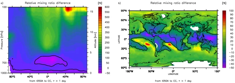
As indicated in Sect. 3, in the previously treated numeri-cal experiments the convective transport is concentrated in a fraction of the grid cell, determined by the convective cloud cover. The current calculation of convective cloud cover in EMAC is rudimentary; assuming that
cconvk = F k up ρairk vupd
, (15)
wherecconv is the convective cloud cover, ρair is the
den-sity of air (in kg m−3), andvupd is the updraft velocity that
Figure 5.Relative difference in zonally and 2001 averaged mixing ratios for UPDP compared to I050A. Results are shown for the tracers with lifetimes of(a)1000 s and(b)1 day.
Figure 6.Relative difference in the 2001 averaged mixing ratio of the atmospheric tracer with a lifetime of 1 day for CC compared to I050A. Results are shown for(a)the zonally averaged data and(b)the difference at the 700 hPa level.
entire grid cell, which is identical to assuming a convective cloud cover of 1. Considering that both settings are possi-ble and that the current calculation of convective cloud cover could be updated, it is worth investigating the impact of this chosen convective cloud cover. To investigate this, numerical experiment CC is performed, which is identical to I050A ex-cept for distributing the convective transport over the entire grid cell.
Due to the larger area, the plumes transport a smaller frac-tion of the affected air mass and there are less recirculafrac-tion effects. Therefore, the vertical transport from the lower cloud layers to the upper cloud layers becomes more effective and especially higher mixing ratios are found in the upper tropo-sphere, as shown in Fig. 6a. In areas of strong convection, this leads to decreased mixing ratios in the lower altitude regions where convective transport is active. This effect is visible from the averaged mixing ratios at a pressure of 700 hPa in
Fig. 6b. Supporting images are presented in Fig. 2 of the Sup-plement. Similar to applying intermediate time stepping, the strongest effects are found for atmospheric tracers with in-termediate lifetimes. The reasons are similar, since the trans-port is affected in the entire plume and the effective verti-cal transport is enhanced. The shift in the tracer lifetime that corresponds with the most pronounced change, towards aτ
of between 6 h and 1 day, is caused by the strongly affected lower part of the convective plumes. For this assumed con-vective cloud cover of 1, enabling intermediate time steps yields smaller differences (RMSD<1 %) due to the weaker local mass transport.
representation of the convective cloud cover when evaluating convective transport.
5 Conclusions and outlook
We presented various modifications to the CVTRANS mod-ule in the EMAC model to update and revise the representa-tion of convective transport of atmospheric compounds. The new, optional functionality consists of (i) intermediate time stepping when updraft mass fluxes are too strong compared to the air mass in individual grid cells, (ii) an analytic ex-pression that accounts for the intra-(sub-)time-step evolution of air properties below the base of the convective plume, and (iii) a recently published parameterization for the mixing ra-tios of atmospheric compounds at the updraft base.
It was demonstrated that applying the intermediate time stepping results in a substantial difference in atmospheric mixing ratios, even when averaged over 2001. The most im-portant effect turned out to be that physical flows no longer need to be capped due to numerical limits. For high values of
fmaxfrac, the effects of air recirculation due to the
compensat-ing subsidcompensat-ing motions in the cloud environment are underes-timated. However, this error is much smaller than that origi-nally introduced by the capping of the physical flows and can be diminished by applying a lowerfmaxfrac. Additionally,
ap-plying the analytic expression accounts for the recirculation around the base of the updraft plume and reduces this error. The updated mixing ratios at the updraft base enhance the efficiency of the convective transport, but the induced devi-ations are of the same order as applying the analytic expres-sion. The magnitudes of all induced differences depend on the lifetime of the evaluated atmospheric compound, which is related to the associated vertical distribution of the tracer and to the regions that are mainly affected by the applied mod-ification. The intermediate time stepping proved most influ-ential for lifetimes on the order of 1 day, while the other two modifications become more influential with shorter lifetimes. Even though the analytic expression and updated plume base mixing ratios are not as important as intermediate time stepping and only result in root mean square deviations in the temporally averaged mixing ratios of less than 1 % of the air-mass-weighted mixing ratios, these improvements come without extra computational cost. Furthermore, these met-rics were determined for averaged mixing ratios over 2001, while local, instantaneous mixing ratios will likely differ more strongly. This will be of importance when comparing model data directly with time-dependent observations. For future numerical experiments we therefore recommend to en-able all three modifications. Only when intermediate time stepping is disabled should the analytic expression not be ap-plied to prevent a further underestimation of the convective transport. The optimal setting offmaxfracdepends on the
se-lected submodels in EMAC. If more computationally expen-sive submodels are enabled, a lowerfmaxfracwill result in
de-creased deviations without a noteworthy increase in compu-tational time. In the evaluated numerical experiment a value of 0.5 was chosen.
As a future development of the convective transport, the current “leaky pipe” representation could be further inves-tigated. In the current implementation, at every individual time step an independent realization of the convective up-drafts and downup-drafts is calculated. This could be updated to a plume that evolves in time, similar to the environmen-tal air. Furthermore, it would be worthwhile to further quan-tify, and subsequently apply, the correct value forfdfor the
various applied numerical grids. Finally, it has been shown that the convective cloud cover representation substantially affects the distribution of atmospheric compounds. Based on Cuijpers and Bechtold (1995), more representative estimates of this convective cloud cover have been proposed (e.g., Neg-gers et al., 2006). However, as discussed by Sikma and Ouw-ersloot (2015), these have to be further adapted. To accu-rately represent convective transport, it will be important to include these updated parameterizations.
Code availability
The Modular Earth Submodel System (MESSy) is being con-tinuously further developed and applied by a consortium of institutions. The usage of MESSy and access to the source code is licensed to all affiliates of institutions that are bers of the MESSy Consortium. Institutions can be a mem-ber of the MESSy Consortium by signing the Memorandum of Understanding. More information can be found on the MESSy Consortium website (http://www.messy-interface. org).
The Supplement related to this article is available online at doi:10.5194/gmd-8-2435-2015-supplement.
Acknowledgements. The authors thank Jordi Vilà-Guerau de
Arellano and Martin Sikma for their feedback during this project. We further wish to acknowledge the use of the Ferret program (http://ferret.pmel.noaa.gov) for graphics in this paper.
The article processing charges for this open-access publication were covered by the Max Planck Society. Edited by: V. Grewe
References
Bechtold, P., Cuijpers, J. W. M., Mascart, P., and Trouilhet, P.: Mod-eling of trade wind cumuli with a low-order turbulence model: toward a unified description of Cu and Sc clouds in meteoro-logical models, J. Atmos. Sci., 52, 455–463, doi:10.1175/1520-0469(1995)052<0455:MOTWCW>2.0.CO;2, 1995.
Cuijpers, J. W. and Bechtold, P.: A simple parameterization of cloud water related variables for use in boundary layer models, J. Atmos. Sci., 52, 2486–2490, doi:10.1175/1520-0469(1995)052<2486:ASPOCW>2.0.CO;2, 1995.
Jöckel, P., Sander, R., Kerkweg, A., Tost, H., and Lelieveld, J.: Tech-nical Note: The Modular Earth Submodel System (MESSy) – a new approach towards Earth System Modeling, Atmos. Chem. Phys., 5, 433–444, doi:10.5194/acp-5-433-2005, 2005.
Jöckel, P., Tost, H., Pozzer, A., Brühl, C., Buchholz, J., Ganzeveld, L., Hoor, P., Kerkweg, A., Lawrence, M. G., Sander, R., Steil, B., Stiller, G., Tanarhte, M., Taraborrelli, D., van Aardenne, J., and Lelieveld, J.: The atmospheric chem-istry general circulation model ECHAM5/MESSy1: consistent simulation of ozone from the surface to the mesosphere, At-mos. Chem. Phys., 6, 5067–5104, doi:10.5194/acp-6-5067-2006, 2006.
Jöckel, P., Kerkweg, A., Buchholz-Dietsch, J., Tost, H., Sander, R., and Pozzer, A.: Technical Note: Coupling of chemical processes with the Modular Earth Submodel System (MESSy) submodel TRACER, Atmos. Chem. Phys., 8, 1677–1687, doi:10.5194/acp-8-1677-2008, 2008.
Jöckel, P., Kerkweg, A., Pozzer, A., Sander, R., Tost, H., Riede, H., Baumgaertner, A., Gromov, S., and Kern, B.: Development cycle 2 of the Modular Earth Submodel System (MESSy2), Geosci. Model Dev., 3, 717–752, doi:10.5194/gmd-3-717-2010, 2010. Kerkweg, A., Sander, R., Tost, H., and Jöckel, P.: Technical
note: Implementation of prescribed (OFFLEM), calculated (ON-LEM), and pseudo-emissions (TNUDGE) of chemical species in the Modular Earth Submodel System (MESSy), Atmos. Chem. Phys., 6, 3603–3609, doi:10.5194/acp-6-3603-2006, 2006. Kim, S.-W., Barth, M. C., and Trainer, M.: Influence of fair-weather
cumulus clouds on isoprene chemistry, J. Geophys. Res., 117, D10302, doi:10.1029/2011JD017099, 2012.
Lawrence, M. G. and Rasch, P. J.: Tracer transport in deep con-vective updrafts: plume ensemble versus bulk formulations, J. Atmos. Sci., 62, 2880–2894, doi:10.1175/JAS3505.1, 2005. Lelieveld, J. and Crutzen, P. J.: Role of deep cloud convection in
the ozone budget of the troposphere, Science, 264, 1759–1761, doi:10.1126/science.264.5166.1759, 1994.
Neggers, R., Stevens, B., and Neelin, J. D.: A simple equilibrium model for shallow-cumulus-topped mixed layers, Theor. Comp. Fluid Dyn., 20, 305–322, doi:10.1007/s00162-006-0030-1, 2006. Nordeng, T. E.: Extended Versions of the Convective Parametriza-tion Scheme at ECMWF and Their Impact on the Mean and Transient Activity of the Model in the Tropics, Tech. Rep. 206, ECMWF, 1994.
Ouwersloot, H. G., Vilà-Guerau de Arellano, J., van Stra-tum, B. J. H., Krol, M. C., and Lelieveld, J.: Quantifying the transport of subcloud layer reactants by shallow cumulus clouds over the Amazon, J. Geophys. Res.-Atmos., 118, 13041–13059, doi:10.1002/2013JD020431, 2013.
Roeckner, E., Brokopf, R., Esch, M., Giorgetta, M., Hagemann, S., Kornblueh, L., Manzini, E., Schlese, U., and Schulzweida, U.: Sensitivity of simulated climate to horizontal and vertical reso-lution in the ECHAM5 atmosphere model, J. Climate, 19, 3771– 3791, doi:10.1175/JCLI3824.1, 2006.
Siebesma, A. P. and Cuijpers, J. W.: Evaluation of parametric assumptions for shallow cumulus convec-tion, J. Atmos. Sci., 52, 650–666, doi:10.1175/1520-0469(1995)052<0650:EOPAFS>2.0.CO;2, 1995.
Sikma, M. and Ouwersloot, H. G.: Parameterizations for convec-tive transport in various cloud-topped boundary layers, Atmos. Chem. Phys. Discuss., 15, 10709–10738, doi:10.5194/acpd-15-10709-2015, 2015.
Tiedtke, M.: A comprehensive mass flux scheme for cu-mulus parameterization in large-scale models, Mon. Weather Rev., 117, 1779–1800, doi:10.1175/1520-0493(1989)117<1779:ACMFSF>2.0.CO;2, 1989.
Tost, H., Jöckel, P., and Lelieveld, J.: Influence of different convec-tion parameterisaconvec-tions in a GCM, Atmos. Chem. Phys., 6, 5475– 5493, doi:10.5194/acp-6-5475-2006, 2006.
Tost, H., Lawrence, M. G., Brühl, C., Jöckel, P., The GABRIEL Team, and The SCOUT-O3-DARWIN/ACTIVE Team: Uncertainties in atmospheric chemistry modelling due to convection parameterisations and subsequent scavenging, Atmos. Chem. Phys., 10, 1931–1951, doi:10.5194/acp-10-1931-2010, 2010.