Technical Note: The normal quantile transformation and its application in a flood forecasting system

(1)

www.hydrol-earth-syst-sci.net/16/1085/2012/ doi:10.5194/hess-16-1085-2012

Earth System

Sciences

Technical Note: The normal quantile transformation and

its application in a flood forecasting system

K. Bogner1, F. Pappenberger2, and H. L. Cloke2,3

1_{Institute for Environment and Sustainability, European Commission Joint Research Centre, Via E. Fermi, 2749,} 21027 Ispra, VA, Italy

2_{European Centre for Medium-Range Weather Forecasts Shinfield Park Reading, Reading, RG2 9AX, UK} 3_{Department of Geography, King’s College London, London, UK}

Correspondence to: K. Bogner ([email protected])

Received: 26 September 2011 – Published in Hydrol. Earth Syst. Sci. Discuss.: 17 October 2011 Revised: 7 February 2012 – Accepted: 22 March 2012 – Published: 2 April 2012

Abstract. The Normal Quantile Transform (NQT) has been used in many hydrological and meteorological applications in order to make the Cumulated Distribution Function (CDF) of the observed, simulated and forecast river discharge, water level or precipitation data Gaussian. It is also the heart of the meta-Gaussian model for assessing the total predictive uncer-tainty of the Hydrological Unceruncer-tainty Processor (HUP) de-veloped by Krzysztofowicz. In the field of geo-statistics this transformation is better known as the Normal-Score Trans-form. In this paper some possible problems caused by small sample sizes when applying the NQT in flood forecasting systems will be discussed and a novel way to solve the problem will be outlined by combining extreme value anal-ysis and non-parametric regression methods. The method will be illustrated by examples of hydrological stream-flow forecasts.

1 Introduction

The Normal Score Transform or NQT has been applied in various fields of geo-science in order to make the mostly asymmetrical distributed real world observed variables more treatable and to fulfil the basic underlying assumption of normality, which is intrinsic to most statistical models (e.g. Moran, 1970; Goovaerts, 1997). For example the meta-Gaussian model is constructed by embedding the NQT of each variate into the Gaussian law (Kelly and Krzysztofow-icz, 1997), which allows the marginal distribution functions of the variates to take any form and the dependence structure

between any two variates to be monotone non-linear and het-eroscedastic. This most convenient property has been in-corporated into the HUP (Krzysztofowicz and Kelly, 2000; Krzysztofowicz and Herr, 2001; Krzysztofowicz and Maran-zano, 2004), which is now part of several operational fore-casting systems (e.g. Reggiani et al., 2009; Bogner and Pap-penberger, 2011) in order to estimate the predictive uncer-tainty of the hydrological forecasts. In Montanari and Brath (2004) and Montanari and Grossi (2008) some problems of the NQT are discussed regarding its limited possibility of making the probability distribution of bivariate random vari-ables multivariate Gaussian. However, Bogner and Pappen-berger (2011) demonstrated that the application of error cor-rection methods could minimize these problems in the case of flood forecasting purposes significantly.

In Van der Waerden (1952, 1953a,b) the theory behind the NQT is outlined and the practical application is demonstrated (e.g. in Krzysztofowicz, 1997; Montanari, 2005; Seo et al., 2006; Todini, 2008). The main objective of this study is to show the difficulties occurring in the inversion of the empiri-cal NQT, if the normal random deviates lie outside the range of the historically observed range, which is particularly im-portant, if this happens during the forecast lead-time.

(2)

Table 1. River Gauging station information for Bohumin and Hofkirchen including stream-flow characteristic value MQ (mean discharge)

and MHQ (average yearly mean discharge).

Station River Area Channel gradient MQ MHQ Latitude Longitude

(km2) (m m−1) (m3s−1) (m3s−1) (◦) (◦)

Bohumin Oder 4350 0.008 40 350 49.92 18.33

Hofkirchen Danube 48 000 0.005 640 1870 48.68 13.11

of the variables by setting the maximum value, for which the probability is assumed to be equal to one, to twice the maxi-mum value of the observed historical maximaxi-mum, resp. to zero for the minimum value, for which the probability is assumed to be null. In Weerts et al. (2011) a linear extrapolation is applied on a number of points in the tails of the distribution. In this study the approach of applying extreme value theory and non-parametric methods will be analysed in more detail. Following the work of Krzysztofowicz (1997) the empiri-cal NQT involves the following steps:

1. Sorting the sample X from the smallest to the largest observation,x(1), ...,x(n).

2. Estimating the cumulative probabilities p(i), ..., p(n) using a plotting position like i/(n+ 1) such that

p(i)=P (X≤x(i)).

3. Transforming each observationx(i)ofX into observa-tiony(i)=Q−1(p(i)) of the standard normal variateY, withQdenoting the standard normal distribution and

Q−1its inverse, applying discrete mapping.

For practical implementation of the methods discussed here, the commands of the freely available and widely used sta-tistical computing language R (R Development Core Team, 2011) are provided in Appendix A (e.g. for computing the steps above).

The problems of applying the NQT arise for the reverse process, when the sampled data points in the normal space fall outside the range of historical samples (i.e. probability quantiles greater thann/(n+ 1) or lower than 1/(n+ 1)).

In order to be able to extrapolate to extreme values, which are rarely observed in the historical samples due to the lim-ited amount of available data, different parametric and non-parametric approaches have been tested in this paper. The problem of a sufficient amount of data is naturally very com-mon for example in flood frequency estimation (Laio et al., 2009), downscaling of climate change scenarios for hydro-logical applications (Bo et al., 2007; Vrac and Naveau, 2007, 2008), and hydrology in general (Zhu, 1987; Engeland et al., 2004). This paper will specifically concentrate on the im-pact of small sample sizes in real-time flood forecasting us-ing ensemble driven systems in combination with the HUP. Further discussion on unrepresentative sample sizes and the

advantage of Bayesian fusion techniques can be found in Krzysztofowicz (2010).

In the next section a forecast example of the European Flood Alert System (EFAS) is shown in order to demon-strate the problem of the back-transformation and its impact on the predictive uncertainty. Then several different solu-tions are given and some advantages and disadvantages out-lined. Finally some concluding remarks and practical advice is given. However only a very limited number of flood events have been observed during the operational run of the post-processor and therefore the evaluation of the forecast quality is rather subjective and has to be analysed in more detail. For example the predictive QQ plot (Laio and Tamea, 2007; Thyer et al., 2009; Bogner and Pappenberger, 2011) could be used to assess whether the time-varying predictive distri-bution of stream-flow is consistent with the observations or similar quantile assessment methods described in Coccia and Todini (2011) could be applied once more forecast data are available.

2 Example forecast

The EFAS (Thielen et al., 2009; Bartholmes et al., 2009) produces daily stream-flow forecasts and includes post-processing through data assimilation and error correction at selected stream-flow gauging stations.

(3)

0

100

200

300

400

500

Time [d]

Streamflo

w [m

3/s]

11/02 03/04 08/05 12/06 05/08

(a) Bohumin

500

1000

1500

2000

2500

3000

Time [d]

Streamflo

w [m

3/s]

10/98 02/00 06/01 11/02 03/04 08/05 12/06

(b) Hofkirchen

Fig. 1. Observed stream-flow and number of clusters exceeding

a threshold at station (a) Bohumin (Odra, CZ) and (b) Hofkirchen (Danube, DE) with 6, resp. 8 yr of daily observations.

fifty years return periods (see Fig. 1). In 2010 during the testing period for the EFAS post-processor, the forecast dis-charge at Bohumin far exceeded the maximum of the histor-ical data sample, and this led to the initiation of this study. Consequently we present the case of Bohumin here. At sta-tion Hofkirchen the effect of sample size on the extrapolasta-tion methods will be analysed in more detail by comparing the re-sults of the total available and a split sample (divided into two halves).

The post-processor runs operationally twice a day and in-cludes the minimization of the error between the most recent past observed and simulated discharge values and the cor-rection of the deterministic ten days ahead forecasts and the corresponding forecasts derived from two different Ensem-ble Prediction Systems (EPS). The NQT is applied prior to the post-processing to all available stream-flow data (mea-sured, simulated and predicted). After the normalization step the differences between observed and simulated stream-flow values are minimized applying the Vector AutoRegressive model with eXogenous input (VARX) to the transformed time series of wavelet coefficients (i.e. fitting the VARX to

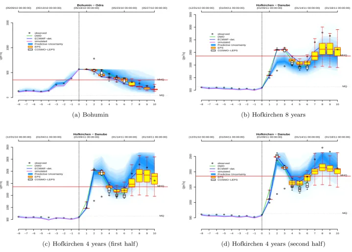
the wavelet transformed series of the observations and sim-ulations simultaneously covering a range of scales). The re-sults of the error corrected predictions are transformed back from normal space into the real world and the predictive un-certainty is estimated (see Bogner and Pappenberger, 2011 for details). In Fig. 2 the final output of the post-processor is shown with forecast initiation at time-step zero (dashed ver-tical line). The past eight days (−8,···,−1) are included to demonstrate the performance of the error correction show-ing the corrected one step ahead predictions, the observa-tions and the prediction uncertainties estimated by the HUP (Krzysztofowicz and Kelly, 2000). From lead-time one on-wards (1, ···, 10) the error corrected forecasts are shown including two stream-flow forecasts based on deterministic weather forecast systems (DWD, ECMWF-det.) and two en-semble prediction systems (51 members EPS from ECMWF and 16 members COSMO-LEPS). The resulting total pre-dictive uncertainty integrating the model input uncertainty (i.e the weather forecast uncertainty) and the hydrological uncertainty is calculated for the different lead-times and is shown as shaded areas. Additionally two thresholds are in-dicated, the MQ value (lower horizontal line) representing the mean daily average discharge and the MHQ (upper hor-izontal line) representing the daily mean annual maximum discharge.

(4)

Bohumin − Odra

Q[m

3/s]

−8 −7 −6 −5 −4 −3 −2 −1 0 1 2 3 4 5 6 7 8 9 10

0

500

1000

1500

observed DWD ECMWF−det. simulated Predictive Uncertainty EPS COSMO−LEPS

(05/09/10 00:00:00) (05/13/10 00:00:00) (05/18/10 00:00:00) (05/23/10 00:00:00) (05/27/10 00:00:00)

MHQ

MQ

(a) Bohumin

Hofkirchen − Danube

Q[m

3/s]

−8 −7 −6 −5 −4 −3 −2 −1 0 1 2 3 4 5 6 7 8 9 10

500

1000

1500

2000

2500

3000

3500

(12/31/10 00:00:00) (01/04/11 00:00:00) (01/09/11 00:00:00) (01/14/11 00:00:00) (01/18/11 00:00:00)

MHQ

MQ

(b) Hofkirchen 8 years

Q[m

3/s]

−8 −7 −6 −5 −4 −3 −2 −1 0 1 2 3 4 5 6 7 8 9 10

500

1000

1500

2000

2500

3000

3500

(12/31/10 00:00:00) (01/04/11 00:00:00) (01/09/11 00:00:00) (01/14/11 00:00:00) (01/18/11 00:00:00)

MHQ

MQ

(c) Hofkirchen 4 years (first half)

Q[m

3/s]

−8 −7 −6 −5 −4 −3 −2 −1 0 1 2 3 4 5 6 7 8 9 10

500

1000

1500

2000

2500

(12/31/10 00:00:00) (01/04/11 00:00:00) (01/09/11 00:00:00) (01/14/11 00:00:00) (01/18/11 00:00:00)

MHQ

MQ

(d) Hofkirchen 4 years (second half)

Fig. 2. Corrected forecast of a flood event without extrapolation in May 2010 at station Bohumin (a), and in January 2011 at Hofkirchen

taking eight years of observation (b), eliminating the first half of the data set (c), eliminating the second half of the data set (d). At station Bohumin (a) and in the second reduced sample at station Hofkirchen (d) the upper limit of applicability is shown, when the maximum of the historical sample is exceeded during the forecast period.

for continental scale forecast systems such as EFAS which runs on a 5 km grid over the whole of Europe.

3 Extrapolation methods

In this paper we concentrate on two approaches which rep-resent a large class of possibilities and allow us to evaluate them in a flood forecasting specific setting:

1. The first method is based on extreme value theory and tries to estimate future possible extreme stream-flow values by fitting a theoretical distribution to the upper (and lower) tail of the sample. The resulting extreme values are combined with the historical sample in or-der to find an optimal transform function. There are multiple approaches which could be used for extrapola-tion based on extreme value theory, for example: nor-mal and nornor-mal distributions and 3-parameter log-normal; Log-Pearson Type III; Extreme Value type I, II, or III; Generalized Extreme Value (GEV); Logistic and

General logistic; Goodrich/Weibull distribution; Expo-nential distribution; or Generalized Pareto Distribution (GPD) – to name a few. More mathematical and sta-tistical details concerning extreme value theory can be found for example in Coles (2001) and Finkenst¨adt and Rootz´en (2004).

(5)

(Lin and Zhang, 1999) and that gave the reason also for choosing the GAM in this study. Many more differ-ent non-linear (regression) models exist, such as neu-ral networks, non-linear prediction methods (e.g. Laio et al., 2003) and kernel based support vector machines (e.g. Yu et al., 2006), but their application is beyond the scope of this technical note. In Fig. 3 some non-linear relationships between the standardized normal observa-tions and the observaobserva-tions are shown demonstrating the appropriateness of GAMs in fitting this non-linear trans-formation function.

3.1 Extreme values

The application of extreme value theory in hydrology has a long tradition and an associated large literature. Fisher and Tippett (1928) started to work on the asymptotic theory of ex-tremes, whereas in Gnedenko and Kolmogorov (1949/1954) the theory for independent identically distributed random variables was completed. Fitting methods of extreme value type distributions to reliability data are outlined thoroughly in the famous work of Gumbel (1958). The Gumbel distri-bution is frequently applied, which is a double exponential distribution representing the limiting distribution for Gaus-sian data. Recently the GEV for annual maxima series (e.g. Ailliot et al., 2011) and the GPD for maxima exceeding thresholds have found the most attraction in environmental extreme value analysis (e.g. MacKay et al., 2011; Moloney and Davidsen, 2011; Mazas and Hamm, 2011).

For the practical implementation in R several packages are available, like “ismev”, “evir” and “POT” (Ribatet, 2006), which has been used in this study. In the Peaks Over Thresh-old (POT) model the limiting distribution of normalised ex-cesses over a threshold converges to the GPD, as the thresh-old approaches the endpoint (Pickands, 1975; Davison and Smith, 1990).

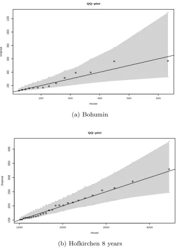
Although Hosking and Wallis (1987) recommended the method of probability weighted moments for small sample sizes, the following two-step approach has been applied here. At first the GPD parameters were estimated by minimiz-ing the Kolmogorov-Smirnov (KS) goodness-of-fit statistics, which were taken in step two as initial values for optimizing the maximum likelihood function by the use of the Nelder-Mead method (Nelder and Nelder-Mead, 1965) resulting in stable parameter estimates and good agreements between the fit-ted and the empirical maxima (Fig. 4). The disadvantage of the POT model is the somewhat subjective choice of a thresholduand the necessity to de-cluster the possible serial correlated time-series by defining some criterion for mak-ing the observed events independent (i.e. definmak-ing the min-imum timespan between two consecutive events not exceed-ing the threshold, see also Bogner et al., 2012, for more de-tails). In the example of R commands given in Appendix A the observed data seriesx is de-clustered first by defining a

0 500 1000 1500 2000 2500 3000

−5

0

5

Streamflow x[m3/s]

Std. Nor

mal Obser

vation y

empirical emp. + POT GAM POT + GAM extrap. GAM extrap. POT

100 200 300 400 500 600

1.0

1.5

2.0

2.5

3.0

Streamflow x[m3/s]

Std. Nor

mal Obser

vation y

(a) Bohumin

0 1000 2000 3000 4000 5000

−6

−4

−2

0

2

4

6

Streamflow x[m3/s]

Std. Nor

mal Obser

vation y

empirical emp. + POT GAM POT + GAM extrap. GAM extrap. POT

1000 1500 2000 2500 3000

01234

Streamflow x[m3 /s]

Std. Nor

mal Obser

vation y

Fig. 3. Normalization of stream-flow values X at station

Bo-humin (a) and at Hofkirchen – 8 yr (b). The range of obser-vations with and without including extreme values (labelled as “emp. + POT”, resp. “empirical”) has been extrapolated applying GAMs.

timespan of eight days to ensure independence of events (see also Fig. 1).

3.2 Nonparametric regression

(6)

200 300 400 500 600

200

400

600

800

1000

1200

QQ−plot

Model

Empir

ical

− − − −− − − − − −

− − −

−

−−− −−

− − −

− −

−

(a) Bohumin

1500 2000 2500 3000

1500

2000

2500

3000

3500

4000

QQ−plot

Model

Empir

ical

−−−−−− − − − −− −

− −− − −− −

− − − − −

− −

−

−−− −− −−

−− −− −− −

−− −−

− −

−

Fig. 4. Resulting QQ plot for the fitted extreme value

distribu-tion (POT Model) versus empirical extreme values including the 95 % confidence interval in gray for Bohumin (a) and Hofkirchen – 8 yr (b).

the range. Within the R package “mgcv” (Wood, 2006) re-cent developments of GAMs have been implemented and the corresponding R function is given in Appendix A.

4 Results

In order to evaluate the dependence of the NQT on the sam-ple size and its effect on the predictive uncertainty based on the meta Gaussian distribution, two different cases have been analysed with respect to (a) extreme values, (b) GAM based and (c) combined extreme values plus GAM based extrapo-lation. The two different cases are:

1. Small sample size (six years) at station Bohumin includ-ing no severe flood events.

2. Sample at station Hofkirchen.

– Covering eight years (i.e. the complete data set available, including severe events).

– After elimination of the first half of the data set (reduced time series excluding most of the severe events, which are concentrated in the first half of the observed data set).

– After elimination of the second half of the data set (most of the severe events remain included). 4.1 Station Bohumin – 6 yr

(7)

Q[m

3/s]

−8 −7 −6 −5 −4 −3 −2 −1 0 1 2 3 4 5 6 7 8 9 10

0

500

1000

1500

(05/09/10 00:00:00) (05/13/10 00:00:00) (05/18/10 00:00:00) (05/23/10 00:00:00) (05/27/10 00:00:00)

MHQ

MQ

(a) Bohumin - including extreme values

Q[m

3/s]

−8 −7 −6 −5 −4 −3 −2 −1 0 1 2 3 4 5 6 7 8 9 10

0

500

1000

1500

(05/09/10 00:00:00) (05/13/10 00:00:00) (05/18/10 00:00:00) (05/23/10 00:00:00) (05/27/10 00:00:00)

MHQ

MQ

(b) Bohumin - GAM

Q[m

3/s]

−8 −7 −6 −5 −4 −3 −2 −1 0 1 2 3 4 5 6 7 8 9 10

0

500

1000

1500

2000

(05/09/10 00:00:00) (05/13/10 00:00:00) (05/18/10 00:00:00) (05/23/10 00:00:00) (05/27/10 00:00:00)

MHQ

MQ

(c) Bohumin - GAM + POT

Fig. 5. Resulting forecast at station Bohumin applying three

differ-ent extrapolation methods: including extreme values based on the POT method (a), fitting the GAM to the historical measurements and linear extrapolation (b), combining the POT and the GAM (c).

extreme values as opposed to the result of extending the sam-ple size with extreme values only without applying GAM, which could result in sharp jumps in uncertainty as soon as the estimated values exceed the historical observed maxi-mum value. In Fig. 5a this drastic discontinuity occurs at

time-step zero (at forecast initiation), where the innermost quantile range (corresponding to the uncertainty range be-tween 0.45 and 0.55 and shown by the darkest shaded area) covers a range of more than 500 m3s−1. Furthermore it can be seen how a slight difference in the stream-flow value in the normal space can cause a big difference in the real world after back-transformation, like the differences in the DWD deterministic forecast (based on weather forecasts provided by the German Weather Service) ranging from 1000 m3s−1 in Fig. 5a and b to 1300 m3s−1in Fig. 5c. However in Fig. 5c it can be seen that the inner quantile ranges (0.35–0.65) cover all the observations in the forecast period (from leadtime 1 to 10) and the predicted median follows quite well the obser-vations, whereas the first two methods result in under or over predictions from a leadtime of three days onwards.

4.2 Station Hofkirchen

The historical data sample at station Hofkirchen comprises eight years and includes several quite severe flood events such as those in May 1999, spring 2002 and August 2002, which correspond to flood events with return periods be-tween 10 and 20 yr (information provided by the Bavarian Environmental Agency). Given this representative data set several tests have been conducted analysing the NQT per-formance and its dependence on sample size and on the ex-trapolation method. Since the majority of the flood events occurred in the first half of the sample (between 1998 and 2003) the NQT and the post-processor have been applied on the total sample and on the split (halved) sample (Fig. 2b– d). Taking the total data set of eight years for calibrat-ing the post-processor results in a forecast with a predictive uncertainty covering almost all the observations, although the first peak of this double-peaked event is overestimated and the second one, the more severe peak, is underesti-mated (Fig. 2b). Nonetheless the observed values of the sec-ond peak fall within the upper quantile range (0.05–0.95) at a leadtime of eight days, which is quite good for a medium range forecast. Fitting the post-processor to the first half of the sample size (Fig. 2c) leads to an increased uncertainty because of the greater variability of the sample. In compar-ison to this the calibration based on the second half sample results in to a forecast with smaller uncertainty bands be-cause of the smaller variance of the sample, demonstrating the importance of sample size and explaining the upper limit of applicability of the NQT, when the observations exceed the historical sample (Fig. 2d).

(8)

Q[m

3/s]

−8 −7 −6 −5 −4 −3 −2 −1 0 1 2 3 4 5 6 7 8 9 10

0

2000

4000

6000

8000

(12/31/10 00:00:00) (01/04/11 00:00:00) (01/09/11 00:00:00) (01/14/11 00:00:00) (01/18/11 00:00:00)

MHQ

MQ

(a) Hofkirchen 4 years (first half, POT)

Q[m

3/s]

−8 −7 −6 −5 −4 −3 −2 −1 0 1 2 3 4 5 6 7 8 9 10

500

1000

1500

2000

2500

3000

(12/31/10 00:00:00) (01/04/11 00:00:00) (01/09/11 00:00:00) (01/14/11 00:00:00) (01/18/11 00:00:00)

MHQ

MQ

(b) Hofkirchen 4 years (second half, POT)

Q[m

3/s]

−8 −7 −6 −5 −4 −3 −2 −1 0 1 2 3 4 5 6 7 8 9 10

1000

2000

3000

4000

5000

(12/31/10 00:00:00) (01/04/11 00:00:00) (01/09/11 00:00:00) (01/14/11 00:00:00) (01/18/11 00:00:00)

MHQ

MQ

(c) Hofkirchen 4 years (second half, GAM + POT)

Fig. 6. Corrected forecast at station Hofkirchen including extreme

values for extrapolation based on (a) four years of the first half, including several severe events and (b) four years of the second half (less severe events) and (c) four years of the second half sample combining the GAM and the POT model for extrapolation.

extreme values fitted to the second half sample results in back-transformed forecast values which substantially exceed the observations because of the discontinuity between the historical data set and the estimated extreme values. Such discontinuities will result in unrealistic, abrupt changes as

can be seen in Fig. 6b at leadtime three and can be cir-cumvented by the application of the GAM in combination with the POT model, which will result in smooth forecasts (Fig. 6c).

5 Conclusions

In this study of the applicability of the NQT in flood forecast-ing systems different problems arisforecast-ing from the small sam-ple sizes are discussed. The chosen forecast examsam-ples at two different stream-flow gauging stations and for two different flood events demonstrate the problems of extending the his-torical data set by extreme values resulting from the fitted POT model. Because of the discontinuity between the ob-served historical sample and the estimated extreme values, sharp and unrealistic rises (or falls) in the hydrograph can occur after transforming the forecast from the Gaussian to the “real world” space. The analysed GAM for approximat-ing the non-linear (back)transformation function could be an alternative, but the problem of possibly unrealistic small pre-dictive uncertainty ranges has to be investigated in more de-tail with longer time-series and at different stations. However for these very limited data sets analysed the suggested way would be the combination of the extension of the small sam-ples by extreme values and the inter- and extrapolation of this prolonged data set by the GAM, which results in smooth forecast hydrographs and not too optimistic under-dispersive predictive uncertainty ranges.

Appendix A

Listing of R commands

# # # # # # # # # # # # #NQT

# S t e p 1 :

x← s o r t ( x )

# S t e p 2 :

p← p p o i n t s ( x , a )}

# w i t h a = 0 f o r t h e W e i b u l l , r e s p . a = 1/

2 f o r t h e Hazen p l o t t i n g p o s i t i o n ) # S t e p 3 :

y←qnorm ( p )

# S t e p 2 and 3 a r e i n t e g r a t e d i n t h e command

y←qqnorm ( x )

# S t e p 4 :

f ←approx ( x , y )

# # # # # # # # # ##

# E x t r e m e v a l u e a n a l y s i s

r e q u i r e ( POT )

e v e n t s ← c l u s t ( x , u=u , t i m . c o n d =8 / 3 6 5 )

mgf . f i t ← f i t g p d ( e v e n t s , t h r e s h =u , e s t =” mgf

(9)

mle . f i t ← f i t g p d ( e v e n t s , t h r e s h =u , e s t =” mle

”, method =” N e l d e r−Mead ”,

c o n t r o l = l i s t ( s t a r t = l i s t ( s c a l e =mgf . f i t $

p a r a [ 1 ] , s h a p e =mgf . f i t $ p a r a [ 2 ] ) )

# # # # # # # # # # # # #GAM

r e q u i r e ( mgcv )

gam . f i t ←gam ( y ∼ s ( x , b s =” c r ”, k = 1 0 ) )

# The s m o o t h t e r m o f t h e o b s e r v a t i o n s x i s s p e c i f i e d by s .

#By s e t t i n g t h e t e r m b s =” c r ” and k =10 t h e p e n a l i z e d c u b i c r e g r e s s i o n s p l i n e # w i l l be a p p l i e d w i t h t h e d i m e n s i o n k o f

t h e b a s i s , u s e d t o r e p r e s e n t t h e s m o o t h t e r m ,

# and w h i c h s e t s t h e u p p e r l i m i t on t h e d e g r e e s o f f r e e d o m

Acknowledgements. The authors wish to thank the Deutsche Wetterdienst, the European Centre for Medium-Range Weather Forecasts, the Bavarian Environment Agency, the Czech Hydrome-teorological Institute (CHMI) and the JRC’s Institute for Protection and Security of the Citizen (IPSC) for data and information. The work was also supported by the UK Natural Environment Research Council (grant NE/I005366/1). Florian Pappenberger is partially funded by GLOWASIS (Global Water Scarcity Information Ser-vice) project (EC, FP7) and DEWFORA (Drought Early Warning Forecasts, EC, FP7). Finally the authors gratefully acknowledge the support of all staff of the JRC’s Institute for Environment and Sustainability (IES) – Land Management and Natural Hazards Unit – FLOODS Action.

Edited by: C. de Michele

References

Ailliot, P., Thompson, C., and Thomson, P.: Mixed methods for fitting the GEV distribution, Water Resour. Res., 47, W0551, doi:10.1029/2010WR009417, 2011.

Bartholmes, J. C., Thielen, J., Ramos, M. H., and Gentilini, S.: The european flood alert system EFAS – Part 2: Statistical skill as-sessment of probabilistic and deterministic operational forecasts, Hydrol. Earth Syst. Sci., 13, 141–153, doi:10.5194/hess-13-141-2009, 2009.

Bo, J., Terray, L., Habets, F., and Martin, E.: Statistical and dynamical downscaling of the Seine basin climate for hydro-meteorological studies, Int. J. Climatol., 1655, 1643–1655, 2007. Bogner, K. and Pappenberger, F.: Multiscale error analy-sis, correction, and predictive uncertainty estimation in a flood forecasting system, Water Resour. Res., 47, W07524, doi:10.1029/2010WR009137, 2011.

Bogner, K., Cloke, H., Pappenberger, F., De Roo, A., and Thielen, J.: Improving the evaluation of hydrological multi-model fore-cast performance in the Upper Danube Catchment, Int. J. River Basin Manage., 10, 1–12, doi:10.1080/15715124.2011.625359, 2012.

Coccia, G. and Todini, E.: Recent developments in predictive uncertainty assessment based on the model conditional pro-cessor approach, Hydrol. Earth Syst. Sci., 15, 3253–3274, doi:10.5194/hess-15-3253-2011, 2011.

Coles, S.: An introduction to statistical modeling of extreme values, Springer series in statistics, Springer, 2001.

Davison, A. C. and Smith, R. L.: Models for Exceedances over High Thresholds, J. Roy. Stat. Soc. B, 52, 393–442, 1990. Deutsch, C. and Journel, A.: GSLIB: Geostatistical Software

Li-brary and User’s Guide, 2nd Edn., Oxford University Press, USA, 1998.

Engeland, K., Hisdal, H., and Frigessi, A.: Practical Extreme Value Modelling of Hydrological Floods and Droughts: A Case Study, Extremes, 7, 5–30, doi:10.1007/s10687-004-4727-5, 2004. Finkenst¨adt, B. and Rootz´en, H.: Extreme values in finance,

telecommunications, and the environment, Monographs on statistics and applied probability, Chapman & Hall/CRC, 2004. Fisher, R. A. and Tippett, L. H. C.: Limiting forms of the frequency

distributions of the largest or smallest member of a sample, Proc. Cambridge Philos. Soc., 24, 180–190, 1928.

Gnedenko, B. V. and Kolmogorov, A. N.: Limit Distributions for Sums of Independent Random Variables, Gosudarstv. Izdat. Tehn.-Teor. Lit., MoscowLeningrad, 1949 in Russian, English transl.: Addison-Wesley, Cambridge, Mass., 1954.

Goovaerts, P.: Geostatistics for Natural Resources Evaluation, Ap-plied Geostatistics Series, Oxford University Press, USA, 1997. Gumbel, E. J.: Statistics of extremes, 2nd Edn., Columbia

Univer-sity Press, New York, 1958.

Hastie, T. and Tibshirani, R.: Generalized Additive Models (with discussion), Stat. Sci., 1, 297–318, 1986.

Hastie, T. and Tibshirani, R.: Generalized Additive Models, Chap-man and Hall, London, 1990.

Hosking, J. and Wallis, J.: Parameter and quantile estimation for the generalized Pareto distribution, Technometrics, 29, 339–349, 1987.

Kelly, K. and Krzysztofowicz, R.: A bivariate meta-Gaussian den-sity for use in hydrology, Stoch. Hydrol. Hydraul., 11, 17–31, 1997.

Krzysztofowicz, R.: Transformation and normalization of variates with specified distributions, J. Hydrol., 197, 286–292, 1997. Krzysztofowicz, R.: Bayesian theory of probabilistic forecasting

via deterministic hydrologic model, Water Resour. Res., 35, 2739–2750, 1999.

Krzysztofowicz, R.: Decision Criteria, Data Fusion, and Prediction Calibration: A Bayesian Approach, Hydrolog. Sci. J., 55, 1033– 1050, 2010.

Krzysztofowicz, R. and Herr, H. D.: Hydrologic uncertainty pro-cessor for probabilistic river stage forecasting: precipitation-dependent model, J. Hydrol., 249, 46–68, 2001.

Krzysztofowicz, R. and Kelly, K.: Hydrologic uncertainty proces-sor for probabilistic river stage forecasting, Water Resour. Res., 36, 3265–3277, 2000.

Krzysztofowicz, R. and Maranzano, C. J.: Hydrologic uncertainty processor for probabilistic stage transition forecasting, J. Hy-drol., 293, 57–73, 2004.

(10)

Laio, F., Porporato, A., Revelli, R., and Ridolfi, L.: A comparison of nonlinear flood forecasting methods, Water Resour. Res., 39, 1129, doi:10.1029/2002WR001551, 2003.

Laio, F., Di Baldassarre, G., and Montanari, A.: Model selection techniques for the frequency analysis of hydrological extremes, Water Resour. Res., 45, W07416, doi:10.1029/2007WR006666, 2009.

Lin, X. and Zhang, D.: Inference in generalized additive mixed modelsby using smoothing splines, J. Roy. Stat. Soc. B, 61, 381– 400, doi:10.1111/1467-9868.00183, 1999.

MacKay, E., Challenor, P., and Bahaj, A.: A comparison of esti-mators for the generalised Pareto distribution, Ocean Eng., 38, 1338–1346, 2011.

Mazas, F. and Hamm, L.: A multi-distribution approach to POT methods for determining extreme wave heights, Coast. Eng., 58, 385–394, 2011.

McCullagh, P. and Nelder, J. A.: Generalized linear models, 2nd Edn., Chapman & Hall, London, 1989.

Moloney, N. and Davidsen, J.: Extreme bursts in the solar wind, Geophys. Res. Lett., 38, L14111, doi:10.1029/2011GL048245, 2011.

Montanari, A.: Deseasonalisation of hydrological time series through the normal quantile transform, J. Hydrol., 313, 274–282, 2005.

Montanari, A. and Brath, A.: A stochastic approach for assess-ing the uncertainty of rainfall-runoff simulations, Water Resour. Res., 40, W01106, doi:10.1029/2003WR002540, 2004. Montanari, A. and Grossi, G.: Estimating the uncertainty of

hydro-logical forecasts: A statistical approach, Water Resources Re-search, 44, W00B08, doi:10.1029/2008WR006897, 2008. Moran, P.: Simulation and Evaluation of Complex Water Systems

Operations, Water Resour. Res., 6, 1737–1742, 1970.

Nelder, J. A. and Mead, R.: A Simplex Method for Function Mini-mization, Comput. J., 7, 308–313, 1965.

Pickands, J.: Statistical inference using extreme order statistics, Ann. Stat., 3, 119–131, 1975.

R Development Core Team: R: A Language and Environment for Statistical Computing, ISBN 3-900051-07-0, R Foundation for Statistical Computing, http://www.R-project.org/, Vienna, Aus-tria, 2011.

Reggiani, P., Renner, M., Weerts, A., and van Gelder, P.: Uncer-tainty assessment via Bayesian revision of ensemble streamflow predictions in the operational river Rhine forecasting system, Water Resour. Res., 45, W02428, doi:10.1029/2007WR006758, 2009.

Ribatet, M. A.: A User’s Guide to the POT Package (Version 1.0), http://cran.r-project.org/ (last access: March 2012), 2006. Seo, D.-J., Herr, H. D., and Schaake, J. C.: A statistical

post-processor for accounting of hydrologic uncertainty in short-range ensemble streamflow prediction, Hydrol. Earth Syst. Sci. Dis-cuss., 3, 1987–2035, doi:10.5194/hessd-3-1987-2006, 2006. Thielen, J., Bartholmes, J., Ramos, M.-H., and de Roo, A.: The

Eu-ropean Flood Alert System – Part 1: Concept and development, Hydrol. Earth Syst. Sci., 13, 125–140, doi:10.5194/hess-13-125-2009, 2009.

Thyer, M., Renard, B., Kavetski, D., Kuczera, G., Franks, S., and Srikanthan, S.: Critical evaluation of parameter consistency and predictive uncertainty in hydrological modeling: A case study using Bayesian total error analysis, Water Resour. Res., 45, W00B14, doi:10.1029/2008WR006825, 2009.

Todini, E.: A model conditional processor to assess predictive un-certainty in flood forecasting, Int. J. River Basin Manage., 6, 123–137, 2008.

Van der Waerden, B. L.: Order tests for two-sample problem and their power I, Indagat. Math., 14, 453–458, 1952.

Van der Waerden, B. L.: Order tests for two-sample problem and their power II, Indagat. Math., 15, 303–310, 1953a.

Van der Waerden, B. L.: Order tests for two-sample problem and their power III, Indagat. Math., 15, 311–316, 1953b.

Vrac, M. and Naveau, P.: Stochastic downscaling of precipita-tion: From dry events to heavy rainfalls, Water Resour. Res., 43, W07402, doi:10.1029/2006WR005308, 2007.

Vrac, M. and Naveau, P.: Correction to “Stochastic downscaling of precipitation: From dry events to heavy rainfall”, Water Resour. Res., 44, W05702, doi:10.1029/2008WR007083, 2008. Weerts, A. H., Winsemius, H. C., and Verkade, J. S.:

Estima-tion of predictive hydrological uncertainty using quantile regres-sion: examples from the National Flood Forecasting System (England and Wales), Hydrol. Earth Syst. Sci., 15, 255–265, doi:10.5194/hess-15-255-2011, 2011.

Wood, S.: Modelling and smoothing parameter estimation with multiple quadratic penalties, J. Roy. Stat. Soc. B, 62, 413–428, 2000.

Wood, S.: Generalized Additive Models: An Introduction with R, Chapman and Hall/CRC, 2006.

Yu, P., Chen, S., and Chang, I.: Support vector regression for real-time flood stage forecasting, J. Hydrol., 328, 704–716, 2006. Zhu, J.: A discussion on the extrapolation of hydrologic series, J.