J. Braz. Comp. Soc. vol.13 número4

Environments Using Mobile Robots

Denis F. Wolf

and Gaurav S. Sukhatme

1

Department Computer Systems Institute of Mathematics and Computer Science

University of São Paulo

P.O.Box 668, Zip 13560-970 São Carlos SP - BRAZIL denis@icmc.usp.br

2

Robotic Embedded Systems Laboratory Department of Computer Science University of Southern California Zip 90089-0781 Los Angeles CA - USA

gaurav@usc.edu

Abstract

Mapping is a basic capability for mobile robots. Most applications demand some level of knowledge about the environment to be accomplished. Most mapping ap-proaches in the literature are designed to perform in small structured (indoor) environments. This paper addresses the problems of localization and mapping in large urban (outdoor) environments. Due to their complexity, lack of structure and dimensions, urban environments presents several difficulties for the mapping task. Our approach has been extensively tested and validated in realistic situ-ations. Our experimental results include maps of several city blocks and a performance analysis of the algorithms proposed.

Keywords: Mobile robotics, Mapping, and Localiza-tion.

1. I

Mapping is one of the most basic capabilities for mo-bile robots. It consists of creating a representation of the environment based on information obtained from sensors. Virtually all sensors have some inherent noise in the data they provide, mapping algorithms have to handle this im-precision, which makes the task even harder. Most map-ping algorithms are designed to operate in small struc-tured (indoor) environments.

Mapping outdoors is considerably more challenging compared to mapping indoor structured environments.

Some of the aspects that make mapping outdoors a hard problem are environment complexity, scale, and terrain roughness.

Most algorithms are designed for mapping indoor spaces generates two dimensional floor plan-like maps, which can fairly represent walls and other features, giv-ing a good idea of how the environment looks like. This type of representation becomes very poor when we try to model more complex environments, which usually have much richer features to be represented (e.g. buildings, trees, and cars on outdoors). A natural extension for 2D maps is to use three-dimensional representations.

Most approaches for indoor mapping deal with office-like spaces while outdoor maps may scale up to city blocks or even more. One of the most frequently used indoor mapping representations is the occupancy grid [6]. While this method is suitable for representing 2D indoor spaces with good accuracy, it does not scale for outdoor spaces.

The terrain is normally flat indoors; this is not the case for most outdoor places. Irregular terrains, depressions and small rocks make the task of mapping a little bit more challenging as they make the robot bump and change its direction, inducing errors in sensor readings and corrupt-ing odometric information.

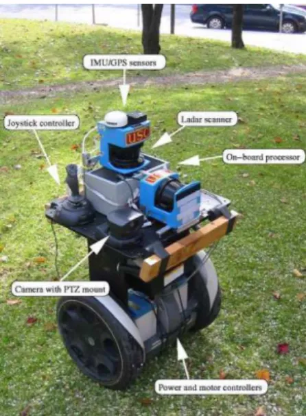
Figure 1. A Segway RMP equipped with laser range finders, GPS, and IMU.

good endurance, can support large payloads, and admits a high vantage point for sensors. One disadvantage of such a robot is that it pitches dramatically when accel-erating and decelaccel-erating. In order to manage that, sen-sor data must be pre-processed using IMU information to compensate the robot’s pitching. Figure 1 shows the Seg-way RMP with a typical mapping setup: an horizontal laser used to do scan matching, a vertical laser used to the mapping task, GPS, and IMU.

The mapping algorithm presented on this section is divided in two phases: localization and mapping. It is also important to mention the constant altitude is assumed for both mapping and localization approaches presented in the next sections.

2. R

W

Outdoor 3D maps have been addressed by the com-puter vision community for many years [12][7]; and also more recently by the robotics community [17] [4]. The approach presented in [7] merges aerial images, airborne laser scans, and images and laser scans taken from the ground. A 2D map is extracted from the aerial images and used along with horizontal laser scans taken from the ground to estimate the robot position during the data ac-quisition. A Monte Carlo method [5] is used to perform the localization task.

Another approach for urban 3D mapping is presented in [9]. In their algorithm a laser range finder pointing up is attached to the roof of a vehicle. As the vehicle moves forward, 3D information is obtained. Feature matching is used to recover the correct position of the robot during the

data acquisition stage.

In the technique presented by [13], 3D geometric models with photometric texture mapping are obtained combining range information with 2D images taken from a mobile platform. In [3], a 3D representation of the en-vironment is obtained from images taken from different poses. In [18] 3D maps are built from the range informa-tion provided by an helicopter.

Many different methods can be used to represent out-door environments. A point cloud is one of the most fre-quently used representation methods. It can describe fea-tures in fine detail when a sufficient number of points is used. On the other hand, this method is not memory effi-cient as it is necessary to store large amounts of data for a detailed representation of large environments.

In order to reduce the complexity of the representa-tions, [14] [10] suggested the use meshes of triangles to model the space. Another efficient mapping representa-tion method is to approximate surfaces by planes. This method has been successfully used in indoor environ-ments [19] [21]. Outdoor environenviron-ments are not always structured; therefore it is somewhat more difficult to ex-tract planes when we have objects like trees, cars, and people in the scene.

3. L

Correct pose estimation is a requirement for mapping. Creating 3D representations for the environment demands 3D localization, which consists of determining the robot’s 6-DOF (degrees of freedom) pose (latitude, longitude, al-titude, roll, pitch and heading). As roll and pitch can be measured directly from the IMU and we assume con-stant altitude, the pose estimation problem is effectively reduced to a 3-DOF problem (latitude, longitude, altitude and heading). We developed two approaches to obtain pose estimation in outdoor environments: GPS-based and prior map-based robot localization.

3.1. GPS-BASEDLOCALIZATION

The particle filter based GPS approximation is based on the particle filter theory. Particle filter is a Bayesian fil-ter that represents the belief by a set of weighted samples (called particles). Particle filters can efficiently represent multi-modal distributions when it is given enough number of particles.

On the mobile robot localization context, each parti-cle represents a possibility of the robot being at a deter-minate position. The particles are propagated as the robot moves. The motion model for the particles is based on the odometer and IMU sensors data. A small amount of gaussian noise is also added to compensate a possible drift in the robot’s motion. The observation model is based on the GPS information. The particles are weighted based on how distant they are from the GPS points. Closer a parti-cle is from the GPS point, higher it is weighted. After be-ing weighted, the particles are resampled. The chance of a particle being selected for resampling are proportional to its weight. High weighted particles are replicated and low weighted particles are eliminated. The complete path of each particle is kept in the memory and at the end only particles that reasonably followed the GPS points will be alive. Consequently, the path of any of these particles can be used as a reasonable trajectory estimation for the robot. Usually, trajectory that had the closest approximation to the GPS points is selected.

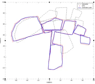
As a result of the GPS based localization, the path es-timated by the particle filter is globally consistent (can close multiple loops) but has a bounded error. It presents some small drifts and a zig-zag effect over the way, caused by the gaussian noise added to the particles. Fig-ure 2 shows GPS data, odometry, and the particle filter-based GPS approximation for the robot’s trajectory.

In order to obtain accurate local pose estimation, a scan matching algorithm is applied after the use of local-ization method described above. Scan matching consists of computing the relative motion of the robot by maximiz-ing the overlap of consecutive range scans. Features like trees, long grass, and moving entities make scan matching a hard task in outdoor environment. In our experiments only linear features have been considered for matching, most of them generated by building structures.

3.2. PRIOR MAP-BASEDLOCALIZATION

The Monte Carlo localization (MCL) algorithm has been proposed by [5] and has been efficiently used on in-door environments. It is also based on a particle filter, but differently from the algorithm proposed in the previous section, the particles are weighted based on the matching of the sensor data and some previous information about the environment. It has the advantage of not requiring GPS information, but on the other hand it requires a prior map of the space. A modified MCL algorithm has also been developed for pose estimation outdoors [11].

Most implementations of the MCL have been used in indoor environments and assume that we have access to both good maps and reliable sensor information, which is not easy to be obtained from outdoors. It is hard to ob-tain accurate maps of outdoors because the environment is very dynamic. There are always people and vehicles moving around and bushes and trees are very hard to be modeled in maps. The measurements provided by range scanners in outdoors are usually much longer than indoor due to the size of the environment; as a result, there is more noise present in the measurements.

Indoor MCL maps typically divide the environment into regions that are either occupied or free. In our case, however, the urban environment is not well mapped, and contains a variety of features that result in unpredictable sensor readings (such as trees, bushes, pedestrians and ve-hicles). We therefore introduce a third type of region into the map: a semi-occupied region that may or may not gen-erate laser returns. Thus, for example, buildings are repre-sented as occupied regions, streets and walkways are rep-resented as free regions, and parking spaces, grass, and gardens as semi-occupied regions. We also assume that semi-occupied regions cannot be occupied by the robot, constraining the set of possible poses. Figure 4 shows a published map of the USC campus, along with the corre-sponding map used by the MCL algorithm (note the semi-occupied regions around most of the buildings).

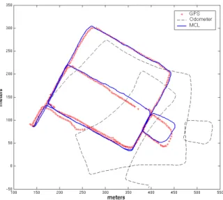
Figure 3 shows the pose estimates generated by the urban MCL algorithm over a tour of the campus. These results were generated by processing the raw data twice: during the first pass, the robot’s initial pose was unknown, and the filter took some time to converge to a singular pose value; once this pose was established, the data was subsequently processed backwards to generate to a com-plete trajectory for the robot. Note that MCL provides pose estimates in areas where GPS is unavailable, and that GPS and MCL estimates are sometimes in disagreement (in this case, visual analysis suggests that it is the GPS estimates that are misleading).

Similarly to the localization method presented in the previous section, the results of the MCL algorithm are globally consistent but not locally accurate. A scan matching algorithm has also been used to obtain fine local pose estimation. The range information is preprocessed and features that can be matched with high confidence like straight lines are extracted. The fact that the Segway RMP pitches considerably during acceleration and decel-eration makes harder the scan matching task.

4. P

C

M

fre-Figure 2. Robot trajectory estimates using particle filter based GPS approximation.

quently used techniques. It can describe features in fine detail when a sufficient number of points is used. These maps can be generated fairly easily when good pose es-timation and range information are available. Based on robot’s position, the environment representation is built directly plotting range measurements into the 3D Carte-sian space.

4.1. POINTCLOUDMAPPINGRESULTS

Figures 5 and 6 shows 3D maps of part of USC cam-pus, the USC Gerontology building, and the USC book-store respectively. Both maps have been built based on range data and the map based localization technique. The data for the USC campus map (Figure 5(a)) was acquired throughout a 2km tour on an area of 115.000m2

. The map has approximately 8 million points. Several loops of different sizes have been traversed during the data acqui-sition step; the localization algorithm efficiently handled the drift in the odometric sensors.

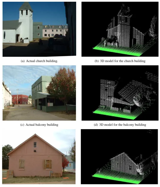
Figure 7 shows some results of mapping experiments performed in Ft. Benning. As there was no previous in-formation about the environment available, the GPS based localization method has been used.

The maps were plotted using a standard VRML tool, which allows us to virtually navigate on the map. It is possible to virtually go on streets and get very close to features like cars and traffic signs and it is also possible to view the entire map from the top.

5. P

M

Compared to point clouds , an efficient mapping repre-sentation method is approximating surfaces present in the

environment by planes. This method has been success-fully used in indoor environments by [19] and [21]. The main idea of this mapping method is to represent build-ings with compact geometric representations. Basically each wall is approximated by one plane. Although these very simple geometric maps do not present the same level of detail as point clouds, they have the advantage of being highly memory efficient. Applications like observabil-ity calculation, path planning, and visualization of large spaces from far away vantage points do not require a high level of detail and the efficiency provided by our approach is very convenient. However, as outdoor environments are not always structured, therefore it is somewhat more dif-ficult to extract planes when we have objects like trees, cars, and people in the scene.

5.1. PLANEEXTRACTION

Figure 3. Robot trajectory estimates using GPS and MCL.

techniques, which just approximate features to points, the Hough transform can handle cases in which multiple or no features fit the points.

A plane in 3D Cartesian space can be expressed as:

d=_xsin_θcos_φ+_ysin_θsin_φ+_zcos_{θ (1)}

where the triplet (d, θ, φ) defines a vector perpendicular to the plane. The distance drepresents the size of this vector and the anglesθandφthe orientation of the vec-tor from the origin [22]. The Hough transform converts a plane in 3D space to ad−θ−φpoint. Considering

a particular pointP (xp, yp, zp), there are several planes

that contain that point. All these planes can be described using equation 1.

Supposing we have a co-planar set of points in 3D and we are interested in finding the plane that fits all of the points in the set. For a specific pointP0(x0, y0, z0) in the set, it is possible to plot a curved surface in thed−θ−

φspace that corresponds to all planes that fitP0. If we repeat this procedure for all points in the set, the curves in thed−θ−φspace will intersect in one point. That

happens because there is one plane that fits all the points in the set. That plane is defined by the value ofd, θ, φon the intersection point. That is how the Hough transform is used to find planes that best fit a set of points in 3D space. However, there are some small modifications to the algorithm that make the implementation much easier and faster, and as a trade-off, the results obtained are less ac-curate. Thed−θ−φspace can be represented as a 3D

array of cells and the curves in that space are discretized into these cells. Each cell value is increased by 1 for ev-ery curve that passes through that cell. The process is re-peated with all curves in thed−θ−φspace. At the end,

the cell that accumulated the highest value represents the space that fits more points. The size of the grid cells cor-responds to the rounding of the value of thed−θ−φ

parameters used to represent planes. The smaller the grid cells used in the discretization the more accurate the pa-rameters that describe planes.

In the case one wants to extract more than one plane from a set of points, every plane for which the correspond-ing cell value is above a determined threshold is consid-ered a valid plane. This is the case in our particular im-plementation.

Since we are fitting planes to point cloud maps, there are cases where there are one or more planes in a set of points. There are also cases where there are no planes at all when the points correspond to non-planar parts of the environment. In order to accommodate these situations, every plane which the correspondent grid cell achieve a determined threshold is considered a valid plane.

5.2. GEOMETRIC REPRESENTATION OF BUILD

-INGS

(a) Scanned map of USC University Park Campus (b) Induced map: free space (white), occupied space (black), and semi-occupied space (gray).

Figure 4. Coarse-scale localization using MCL. The particle filter estimate is indicated by the arrow.

(a) Part of USC campus, the gray line corresponds to the trajectory of the robot during the mapping.

(b) 3D map of part of USC campus.

(a) USC Gerontology building (b) 3D map of USC Gerontology building.

Figure 6. USC Gerontology building and the corresponding 3D model.

approximated by 5 planes (4 lateral planes and one top plane), which corresponds to 8 points in 3D space. It is important to mention that this compactness in the repre-sentation may result in a considerable lose of details.

Extracting planes from indoor environment point clouds is a relatively easy task once most of the internal parts of built structures are flat surfaces. In outdoor urban environments it can be much harder due to the presence of various elements that are not part of buildings like trees, bushes, people, and vehicles. On many occasions, these elements cause occlusion of part of the building struc-tures. The closer to the sensors these obstaclesare the larger the occluded area is.

Another issue in extracting planes from 3D points is that distant points originated by different features may align, inducing the presence of large planar structures when using Hough transform. In order to handle these situations, our approach divides the point cloud into small sections of 3D points. These sections overlap each other to guarantee that plane surfaces are not broken into two pieces. As a result we have a large set of small planes.

After extracting planes from building structures, it is necessary to combine them in order to represent build-ing structures. On our implementation we make the as-sumption that valid building walls are vertical or hori-zontal with a small tolerance. This assumption simplifies not only the extraction of planes but also their combina-tion. With few exceptions, this assumption holds for most cases in our experiments. As a result of this assumption, the search space of the Hough transform will be smaller, making the plane extraction process faster and the associ-ation of planes easier.

The algorithm proposed by [15] has been used to com-bine planes. This algorithm efficiently merges line

seg-ments (in our case planes) that are close of each other and have similar directions. It handles both overlapping and non-overlapping segments, weighting (calculating the rel-ative importance) the segments according to their size.

5.3. PLANARMAPPINGRESULTS

The mapping approach described above have been tested during experiments in the USC campus and Ft. Benning/GA. The platform used during the experiments was a Segway RMP with SICK laser range finders, IMU, and GPS. Player/Stage has been used as a software con-troller. The robot mapped part of Ft. Benning in an ap-proximately 1km tour with an average speed of 1.2m/sec. At the USC campus, the point cloud was generated using the map based localization technique and the pla-nar mapping algorithm has been was applied to create the building model. During the mapping task, the robot made a complete loop around the USC accounting building. This example is particularly challenging because there were many trees and bushes between the robot and the building. These obstacles occluded a considerable part of the building walls. The actual building can be seen in Figure 8 (a) and the point cloud representation is shown in Figure 8(b). The planar model of the accounting building is shown in Figure 8(c).

During our experiments in Ft. Benning, the robot mapped an area of 120m X 80m, over a run of more than 1.5km. The maps have been manually placed over an aerial picture, taken by an UAV developed at the Uni-versity of Pennsylvania, GRASP Laboratory (under the DARPA MARS 2020 project collaboration)[20].

(a) Actual church building. (b) 3D model for the church building

(c) Actual balcony building (d) 3D model for the balcony building

(e) Actual house (f) 3D model for the house

Figure 7. 3D maps of Ft. Benning based on pose estimation and range data.

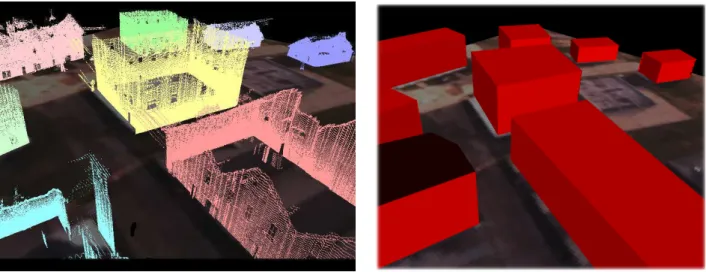
(a) Actual building (b) Point cloud (c) Planar model

(a) Ft. Benning MOUT Site from the top. (b) Closer view of the Ft. Benning MOUT Site 3D map.

Figure 9. 3D maps of Ft. Benning built based on pose estimation and range data.

(a) Ft. Benning MOUT Site from the top. (b) Closer view of the Ft. Benning MOUT Site 3D map.

very rough making the robot’s internal odometer drift, the pose estimation algorithm successfully corrected those er-rors. Figures 9 and 10 show the point cloud and planar mapping results.

Unfortunately, there was no ground truth available to estimate the absolute error in the map representation. However, visually it is possible to note a small misplace-ment between the planar building structures and the aerial UAV picture.

6. C

F

W

This paper addressed the problem of mapping and lo-calization in large urban environments We proposed two algorithms for localization (gps-based and map-based) and two map representations (point cloud and planar). As there was no ground truth available, the performance anal-ysis of the algorithms has been done based on GPS infor-mation. As it is showed in the Sections 4 and 5, our algo-rithms are capable to build detailed and globally consis-tent maps of large urban environments. Our experimental tests performed at USC campus and Fort Benning show the details of the point cloud and the efficiency and com-pactness of the planar representations.

As a future work we plan to use other types of sen-sors and integrate them using other techniques to better estimate robot’s pose during the data acquisition. We also plan to use images provided form video cameras to add texture to planar models, which would lead to even more realistic maps.

Acknowledgments

This work is supported in part by NSF grants IIS-0133947, CNS-0509539, CNS-0331481, CCR-0120778, and by the grant 2005/04378-1 from FAPESP-BRAZIL.

R

[1] A. Bartoli. Picewise planar segmentation for auto-matic scene modeling. InIEEE International Con-ference on Computer Vision and Pattern Recogni-tion, page 2001, 283-289.

[2] J. Bauer, K. Karner, k. Schindler, A. Klaus, and C. Zach. Segmentation of building models from dense 3d point-clouds. InWorkshop of the Austrian Association for Pattern Recognition, 2003.

[3] M. Bosse, P. Newman, L. John, M. Soika, W. Feiten, and S. Teller. An atlas framework for scalable map-ping. InInternational Conference on Robotics and Automation, pages 1899–1906, 2004.

[4] C. Brenneke, O. Wulf, and B. Wagner. Using 3d laser range data for slam in outdoor environments. InIEEE/RSJ International Conference on Intelligent Robots and Systems, pages 18–193, 2003.

[5] F. Dellaert, D. Fox, W. Burgard, and S. Thrun. Monte carlo localization for mobile robots. InIEEE International Conference on Robotics and Automa-tion, pages 99–141, 1999.

[6] A Elfes. Sonar-based real-world mapping and navi-gation.IEEE Transactions on Robotics and Automa-tion, 3(3):249–265, 1986.

[7] C. Fruh and A. Zakhor. Constructing 3d city models by merging aerial and ground views. IEEE Com-puter Graphics and Applications, 23(6), 2003. [8] N. Guil, J. Villaba, and E. Zapata. A fast hough

transform for segment detection.IEEE Transactions on Image Processing, 4(11), 1995.

[9] Zhao H. and R. Shibasaki. Reconstructing urban 3d model using vehicle-borne laser range scanners. In

3rd. International Conference on 3D Digital Imag-ing and ModelImag-ing, 2001.

[10] D. Haehnel, W. Burgard, and S. Thrun. Learning compact 3d models of indoor and outdoor environ-ments with a mobile robot.Robots and Autonomous Systems, 44:15–27, 2003.

[11] A. Howard, D. F. Wolf, and G. S. Sukhatme. To-wards autonomous 3d mapping in urban environ-ments. InIEEE/RSJ International Conference on In-telligent Robots and Systems, pages 419–424, 2004. [12] J. Hu, S. You, and U. Neumann. Approaches to large-scale urban modeling.IEEE Computer Graph-ics and Applications, pages 62–69, 2003.

[13] M. K. Reed and P. K. Allen. 3-d modeling from range imagery: an incremental method with a plan-ning component. Image and Vision Computing, 17:99–111, 1999.

[14] Y. Sun, J. K. Paik, Koschan. A., and M. A. Abidi. 3d reconstruction of indoor and outdoor scenes using a mobile range scanner. InConf. on Pattern Recogni-tion, pages 653–656, 2002.

[15] J. M. R. S. Tavares and A. J. Padilha. New approach for merging edge line segments. In7th. Portuguese Conference of Pattern Recognition, 1995.

[17] S. Thrun, W. Burgard, and D. Fox. A real-time algo-rithm for mobile robot mapping with applications to multi-robot and 3d mapping. InIEEE International Conference on Robotics and Automation, 2000. [18] S. Thrun, M. Diel, and D. Haehnel. Scan alignment

and 3d surface modeling with a helicopter platform. In International Conference on Field and Service Robotics, 2003.

[19] S. Thrun, C. Martin, Y. Liu, D. Haehnel, R. E. Mon-temerlo, D. Chakrabarti, and W. Burgard. A real-time expectation maximization algorithm for acquir-ing multi-planar maps of indoor environments with mobile robots. Transactions on Robotics and Au-tomation, pages 433–442, 2004.

[20] UPENN/GRASP. Aerial view of Ft. Benning taken by an UAV., Personal communication, September 2005.

[21] J. W. Weingarten, Gruener G., and R. Siegwart. Probabilistic plane fitting in 3d and an application to robotics mapping. InIEEE International Confer-ence on Robotics and Automation, pages 927–932, 2004.