P. R. Barbosa and
P. Seleghim Jr.
Núcleo de Engenharia Térmica e Fluidos Departamento de Engenharia Mecânica Escola de Engenharia de São Carlos Universidade de São Paulo – USP Av. Trabalhador Sãocarlense, 400 13566-590 São Carlos, SP. Brazil paulorb@sc.usp.br and seleghim@sc.usp.br
Improving the Power Consumption in
Pneumatic Conveying Systems by
Adaptive Control of the Flow Regime
The pneumatic conveying of solids in a gas stream is a recurrent process in petrochemical industries. However, due to practical limitations the majority of existing systems have capacities ranging from 1 to 400 tones per hour over distances less than 1000 m, mainly because of a high power consumption per transported unit mass. More specifically, to avoid the formation of dense structures such as dunes and plugs, which, depending on the characteristics of the material and on the availability of a pressure head from the carrier phase may cause a violent pressure surge or a possible line blockage, the system is preferably operated at homogeneous dispersed flow. To sustain such a flow regime high velocities are needed and, accounting for the resulting higher pressure drops, higher power consumption is demanded. An optimized pneumatic conveying system can be conceived with the help of adaptive control techniques. In the context described above, lower transport velocities are allowed if the formation of aggregates that precedes the transition to dense phase flow regimes are automatically detected and destroyed, thus, artificially stabilizing the light phase homogeneous flow regime. This work assesses the reduction in the necessary power that the application of such adaptive control technique could produce. Experimental results are presented for a 45 mm i.d. pneumatic conveying system used to transport Setaria Italica seeds. The instrumentation used to identify the flow regime is constituted of several pressure sensors installed along the transport line. The proposed control strategy is based on processing these signals through a neural network model to assess the flow condition and to mimic an optimized gain scheduled PID algorithm. Preliminary results show that reductions in power consumption can reach 50% when compared with classical non controlled transport.
Keywords: Pneumatic conveying, control, neural network, gas-solid flow
Introduction
The pneumatic conveying of solids in a gas stream is a recurrent process in petrochemical industries, mainly because of its flexibility, security in the transport of high valued products, ease of automation/control and low maintenance costs. The range of material that can be pneumatically transported is extensive: powders and rocks of up to 50 mm in size to finished manufactured parts such as electronic components for instance. However, due to practical limitations the majority of existing systems have capacities ranging from 1 to 400 tones per hour over distances less than 1000 m and average particulate size less than 100 mm. Among these limitations probably the most important one refers to a high power consumption per transported unit mass. More specifically, to avoid the formation of dense structures such as dunes and plugs, which, depending on the characteristics of the material and on the availability of a pressure head from the carrier phase may cause a violent pressure surge or a possible line blockage, the system is preferably operated at homogeneous dispersed flow. To sustain such a flow regime high velocities are needed (15 to 20 m/s for instance) and, accounting for the resulting higher pressure drops, higher power consumption is demanded. Another important problem associated with the increase in the transport velocity is the abrasion of the equipment and degradation of the transported particulate.1
From a phenomenological point of view, pneumatic transport can be seen as a special application of gas-solid flows which can be described with the help of the so called state diagram, i.e. the curves of specific pressure drop in function of the gas superficial velocity. It is also possible to define a state diagram by plotting mass flow ratios in terms of the Froude number, which is a more general and convenient representation of the phenomenon. Either way, gas-solid flow state diagrams indicate that the transition from dispersed (or
Paper accepted August, 2003. Technical Editor: Aristeu da Silveira Neto.
light) type flows to dense phase flows is associated to a minimum in the specific pressure drop, which would be an ideal operating condition if the above mentioned problems could be avoided.
In more specific words, the problem of operating the transport line near transition velocities lies on the hysteretic behavior of the transition. This can be better understood through a test on a horizontal line where the velocity of the carrier phase is slowly varied between zero and a maximum value, above which the flow regime is dispersed and does not change. The different stages of this experiment are indicated in figure 1, where the flowing particles velocity Up is plotted against the gas velocity Ug. In stage (a) Ug is not sufficiently high to levitate the particles so Up = 0 until a critical value is reached (Ug = U1). After this, in stage (b), Ug > U1, the particles are entrained by the gas flow and fully dispersed regime is asymptotically reached (Upo Ug). From a maximum gas velocity value, Ug is decreased in stage (c) of the experiment and different flow regimes may appear, such as stratified flow, intermittent flow
Figure 1. Schematic representation of the different flow regimes in horizontal gas-solid flow when varying the carrier velocity.
Gas Velocity (U )g
U2
(a) U
1
(b)
(c)
U3
P
a
rt
ic
le
V
e
lo
c
it
y
(U
and dune flow, until another critical value Ug = U2 is reached. At this point particles are no longer sustained in the core, some of them will segregate and stop and others will roll and bounce over the fixed particle layer at Up = U3. Operating the transport line near the light-dense transition means setting Ug to lay between U1 and U2 and handling a strong hysteretic behavior of Up as well as of the pressure drop and other relevant macroscopic parameters. Therefore, the safe operation within these conditions requires special control strategies, which is one of the main objectives of this work.
This work assesses the reduction in the necessary power that the application of such adaptive control technique could produce. Experimental results are presented for a 45 mm i.d. pneumatic conveying system used to transport Setaria Italica seeds (bird seed). The proposed control strategy is based on a neural network model responsible for both assessing the flow condition and for reproducing an optimized gain scheduled PID algorithm. Preliminary results show that reductions in power consumption can reach 50% when compared with classical non controlled pneumatic transport.
Nomenclature
D = pipe inner diameter Dp = avarege particle diameter e = power optimization factor E = penalty function fi = activation function Fr = Froude number
g = gravitational acceleration H = total number of interconnections Kd = derivative gain
Ki = integral gain Kp = proportional gain mg = gas flow rate ms = solids flow rate
N = nominal operating condition O = optimized operating condition pi = neural network input
Pi = static pressures
qi = desired neural network output ri = neural network output
T = transition line Ug = gas velocity Up = particle velocity U1, U2, U3 = critical velocities wi,j = neural network weigth
Wadaptive = power consumed with adaptive control Wnom = power consumed without adaptive control xi = input of the i-th neuron
yi = output of the i-th neuron Greek Symbols
G,F = exponent in Marcus equation
¨mg=gas flow rate correction
¨ms = solid flow rate correction P = mass flow ratio
Us=solid density
Neural Network Models
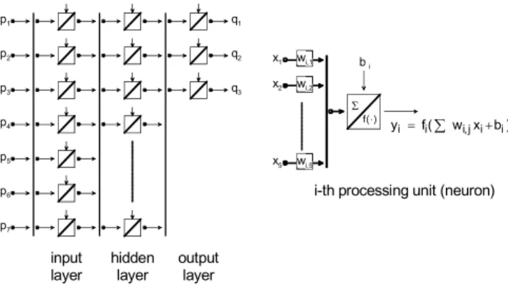
From a functional point of view a neural network model can be defined as a large number of simple interconnected processing units used to establish an input/output relationship, and for which most of the stored information is associated to the strength of the interconnections. A typical processing unit, or neuron as it is called in the jargon, produces a scalar output by applying an activation
function to a biased weighted sum of its inputs. In other terms, if yi and xi,jrepresents respectively the output and the inputs of the i-th neuron, fi() its activation function, wi,j the corresponding weighting coefficients and bi a bias coefficient, the input/output relationship is given by
y = f ( jw x + b )
i i ¦ i,j i,j i (1)
A typical feed-forward multi-layer network is then formed by interconnecting several neurons and, consequently, defining a formal relationship between an input vector { pi } and an output vector { qi }, as depicted in figure 2.
Figure 2. Schematic representation of a feed-forward neural network with
3 layers (input, hidden and output ) and generating 3 output values { qi }
from 7 input values { pi }. The number of neurons at the input and output
layers is generally taken to be equal to the number of input and output values respectively.
One of the most important features of a neural network model is its ability to store input/output patterns, the so-called associative memory, and to produce similar outputs from similar input patterns, the projection property. This can be done by properly adjusting the weighting coefficients according to a given learning heuristics, such as the supervised back-propagation method adopted in this work. In more precise terms, consider a learning data set of input/output pairs ( { pi }n , { qi }n) , where n = 1,2...N. and also weighting coefficients { wi,j }k, in which the subscript k will stands for the adjustment cycle (or epochs as it is called). During the adjustment process, the application of the inputs { pi }n will produce outputs { ri, }n,k progressively closer to { qi }n , i.e. the desired ones. The process can be formulated as an optimization problem with a penalty function defined as
N 2
i,j k i n i n,k
n=1 1
E { w } = { q } - { r }
2
ª º
¬ ¼
¦
(2)This is clearly a continuous differentiable function of the weights { wi,j }k and, thus, a classical gradient descent method can be applied to determine the set { wi,j }f which minimizes (2). This is the essence of the back-propagation method, although there are crucial details regarding the choice of the activation functions and the strategy of updating { wi,j }k. A detailed discussion of this can be found in Hertz et al. (1991). The performance of a neural network is profoundly affected by its internal architecture (the number of hidden layers and the number of neurons in each one) and the type of interconnections (feed-forward, recursive, winner-take-all, etc.). Despite this, there is no general mathematical theory but rather a number of empiric rules to be considered when constructing such models (Crivelaro et al., 2002).
6
x1
x2
x5
b i p1
p2
p3
p4
p5
p6
p7
q1
q2
q3
¦w xb) (
f
yi i ,ij i i
) ( f wi,1
wi,2
wi,5
i-th processing unit (neuron)
input layer
hidden layer
Regarding the problem of controlling gas-solid flow regimes, somewhat analogous to the problem of recognizing characters from a scanned text for which there is a well established knowledge base, a modular architecture presents advantages over a fully interconnected model (see for instance Cao et al., 1996, or Gader et al., 1996). In particular, empirical estimations indicate that the learning time on a conventional single processor computer depends approximately on H3 (the total number of interconnections to the third). Thus, the decomposition of the global network into independent modules facilitates the rapid and efficient adjustment of the weighting coefficients. It is thus convenient to adopt a model based on two independent neural networks, the first one responsible for assessing the flow regime by defining proper target and gain values for the controller, the second one dedicated to the calculus of the flow rate corrections in order to have optimal flow conditions. This architecture is depicted in figure 3, in which mg, ms,¨mg and
¨ms stands for the gas and solids flow rates and their corrections respectively, Pi (i = 1,2,...M ) denotes the static pressure measured along the transport line, d is the target value and KP, KI and KD are the proportional, integral and derivative gains. Before entering in further details on how these variables are processed, it is convenient to present the proposed control strategy.
Figure 3. Controller internal architecture defined in terms of two independent neural network models.
Gain Scheduled Control Strategy for Pneumatic
Transport
The automatic change in the parameterization of a process controller is known as gain scheduling. Discretely scheduled PID algorithms and linear controllers with a statistical approach to schedule its internal parameters correspond to different realizations of the same concept. Generally, scheduled control algorithms are used as linear compensation for processes with known non-linearities when auxiliary measurements are available that correlate well with the system dynamics (Doyle et al., 1998). As it was discussed above, this is exactly the case in pneumatic transport when operating near the light-dense flow transition and could be thus adopted in this work. Alternative strategies, mostly based on nonlinear control, although its recent advances, often lead to controllers of very complex structures (Knoop and Perez, 1994) and often lacking the necessary robustness to be applied in an industrial process (Doyle et al., 1989).
In view of this, the successful use of a scheduled gain control strategy in a solids pneumatic conveyor requires additional process variables to assess the non-linearities of the system dynamics, i.e. the dynamics of the flow regime transition and, also, the possibility to adjust optimum non-scheduled PID controllers which are specific for different flow regimes. The first condition can be straightforwardly fulfilled through the state diagram of the transport system, which justifies the choice of the input variables as shown in figure 3 (gas and solids mass flow rates and static pressure along the transport line). The fulfillment of the second condition was the object of a previous research work (Schiavon, 2000), in which
optimal PID controllers were tuned, i.e. optimum KP, KI and KD values were determined, around specific operating states of a 45 mm internal diameter 3 m long pneumatic transporter, using 0.8 mm average diameter sand particles (an analogous situation to the one treated in this work).
Consider then, the generic state diagram shown in figure 4, which is very similar to the one constructed for the test loop used in this work and described in details in the following section. The dotted line (T) indicates the frontier between dense and light phase flow regimes. The continuous inclined lines represent the constant solids mass flow rate lines plotted according to the corresponding mass flow ratio P, defined as
s
g m =
m
P (3)
and to the Froude number Fr defined as
g U
Fr =
D g
(4)
where D is pipe internal diameter and g denotes the gravitational acceleration. The other two dotted lines, indicated by (O) and (N) in figure 4, represent the loci of the specified operating condition with and without adaptive control of the flow regime. More exactly, (O) represents the optimized operating condition, defined by setting Ug to be approximately 5% higher than the transition velocity, while (N) represents the nominal condition determined by imposing Ug to be 2 or 3 times higher than the transition velocity (18 m/s for the particulate used in this work, according to Marcus et al., 1990).
Figure 4. Schematic representation of a state diagram for a pneumatic
transport line in terms of the mass flow ratio P and the Froude number Fr.
Within this framework, and considering the objective of minimizing the power consumption associated to the transport process, the variable d quantifies an abstract distance or error between the optimum and the actual flow regime and, thus, should be kept as closest to zero as possible. The way this should be done is implemented through the internal parameterization of the controller, which should be scheduled to cope the differences associated with the flow regimes. If the operating point lies below the optimum line (O), i.e. d > 0 as indicated in figure 4, the flow regime is dispersed and smooth corrections are required to bring d back to zero. Usually in this flow condition, KD is tuned at relatively high values in order to produce an asymptotic trajectory back to (O) to avoid overshoots.
mg
ms
P1
P2
PN
d
flow regime neural model Kp
KI
KD
'mg
'ms
control neural model
log (Froude number) dense phase
ms = cte
light phase
(T)
(O)
(N)
d
lo
g
(m
a
s
sf
lo
w
ra
ti
o
10 12 14 16 18 20 22 24 2
3 4 5 6 7
T 0.0739 kg/s
0.1037 kg/s 0.1228 kg/s 0.1343 kg/s 0.1395 kg/s 0.1437 kg/s
ms
Mass flo
w ratio
Froude number If the operating point lies within (O) and (T), that is d < 0 but d | 0,
a fast correction is needed and some overshooting is allowed or even desired. To reproduce this behavior KP must be comparatively big and KD| 0. For the last, if the operation point lies above (T), the flow regime is dense and the transport line is possibly blocked. Special procedures should be triggered in order to protect the equipment and to restart the process again.
Figure 5. Schematic representation of the pneumatic transport test loop at the NETeF – USP.
The main advantage of using neural network models is that such a complex control strategy can be easily implemented by adjusting their internal weighting coefficients and bias, according to a training rule such as the supervised back-propagation method for instance. Another important advantage is that the variable d does not need to be explicitly calculated from the input variables. Applying an on-site calibration technique (Rolnik and Seleghim, 2002) the controller can gain knowledge of the loci of the optimum operation points (line (O) ), through which d can be reproduced directly from the corresponding flow rates and pressures. In other words, the neural model will work as a nonlinear fit between the input and output variables.
The Test Facilities and the Test Grid
The validation tests were done at the experimental facilities of the Thermal and Fluids Engineering Laboratory of the University of São Paulo at São Carlos (NETeF-USP). The pneumatic transport loop, drawn schematically in figure 5, has a transparent 45 mm inner diameter test section, extending horizontally through 12 m and vertically through 9 m. Air is supplied by a 60 hp screw compressor (1), capable of generating air speeds up to 40 m/s in the transport line. The air flow rate is controlled with the help of a servo-valve (2) and measured by an orifice plate (3), instrumented with temperature and pressure transmitters (differential and absolute). The particulate is introduced in the transport line through a venturi feeder (4), which receives the particulate from a screw conveyor (5). The solids flow rate is controlled by imposing the rotation of the screw conveyor with a frequency converter (6). A cyclone separator (7) is placed at the exit of the test section, from where the particulate may be returned to a separated storage container (8) for batch operation or, alternatively, to a rotary airlock (9) connected to the feeding silo (10) for continuous operation.
The particulate used in the tests was Setaria italica seeds with an average diameter DP = 2.5 mm and an approximately density of
800 kg/m3. Several steady state experiments were done with
different combinations of gas and solids mass flow rates resulting in
P ranging from 1.99 to 6.15 and Fr ranging from 18.4 to 29.2. In dimensional units this corresponds to mg between 79.6 and 133 kg/h, and ms between 158 and 820 kg/h. The transition line (minimum pressure drop line) agrees extremely well with the following correlation proposed by Marcus et al. (1990)
- Ȥ
= 10G Fr
P (5)
in which the exponents G and F are calculated from the average particle diameter (in mm) according to
P
= 1.44 D + 1.96
G (6)
2.5 D 1.1
Ȥ P (7)
The test data points and the corresponding transition line are plotted in figure 6.
Figure 6. State diagram and corresponding transition and constant solids mass flow rate lines.
Power Optimization Results
By controlling the flow regime it is possible to operate near the dense-light transition line and obtain a significant reduction in the power needed to transport a given solids charge. To be able to quantify this, a power optimization factor was defined according to the following expression
nom adaptive
nom
W - W
e =
W
(8)
in which Wnom and Wadaptive indicate the necessary power
respectively without and with adaptive control of the flow regime. These powers were calculated by assuming isothermal flow (RT = constant) and imposing energy balance, that is
1 g
N P
W = m R T ln
P
§ ·
¨ ¸
© ¹ (9)
where P1 is the pressure at the inlet of the test section (1.5 m downstream from the solids feeder) , and PN the pressure at its outlet (1.5 m upstream from the cyclone).
technique may result in power savings around 50%, for the experimental conditions of this work
Table 1. power optimization results calculated according to (8) and obtained at different constant solids mass flow rates.
m
s(kg/s)
W
nom(kW)
W
adaptive(kW)
e (%)
0.0739 2.63 1.34 48.91
0.1037 3.15 1.56 50.68
0.1228 3.23 1.63 49.45
0.1343 3.06 1.55 49.34
0.1395 2.99 1.54 48.60
0.1437 3.12 1.42 54.49
Conclusions and Perspectives
A technique for the adaptive control of gas-solids flow regimes occurring in pneumatic transport systems was proposed in this work. The control algorithm is based on two independent neural models, the first one being responsible for assessing the flow regime by defining proper target and gain values for the controller, the second one mimics an optimized gain scheduled PID loop and is dedicated to the calculus of the flow rate corrections in order to have optimal flow conditions. This technique allows the operation near the minimum pressure drop line in the state diagram and a significant reduction in the power consumption for the same solids charge, when compared with a non-controlled system operating at fixed nominal conditions. This is so because without adaptive control the carrier phase velocity must be 2 or 3 times higher than the light to dense phase transition to avoid the formation of dense structures such as dunes and plugs, which, depending on the characteristics of the material and on the availability of a pressure head from the carrier phase may cause a violent pressure surge or a possible line blockage. Experimental testes performed with Setaria italica seeds in a 45 mm i.d. pneumatic conveying line show that the proposed control technique is capable of producing power optimization
factors of up to 50% approximately. Future work should include systematic experimental tests, with different types of particulate and extended flow rate ranges, in order to assess the applicability of the proposed control technique in industrial processes.
Acknowledgements
The authors would like to acknowledge the financial support provided by FAPESP thought grant 02/00472-5, and by CNPq through grant 62.0012/99-4.
References
Cao, J., Ahmadi, M.. and Shridhar, M.., 1996, “A hierarchical neural network architecture for handwritten numerical recognition”, Pattern recognition, Vol. 30, No. 2, pp. 289-294.
Crivelaro, K.C.O., Seleghim Jr., P. and Hervieu, E., 2002, “Detection of horizontal two-phase flow patterns through a neural network model”, Journal of the Brazilian Society of Mechanical Sciences, Vol. XXIV, No. 1, pp. 70-75.
Doyle III, F.J., Packard, A.K. and Morari, M., 1989, “Robust controller design for a nonlinear CSTR”, Chemical Engineering Science, Vol. 44, No. 9, pp.1929-1947.
Doyle III, F.J., Kwatra, H.S. and Schwaber, J.S., 1998, “Dynamic gain scheduled process control”, Chemical Engineering Science, Vol. 53, No. 15, pp. 2675-2690.
Gader, P.D., Mohamed, M.A. and Keller, J.M., 1996, “Fusion of handwritten word classifiers”, Pattern Recognition Letters, Vol. 17, pp. 577-584.
Hertz, J., Krogh, A. and Palmer, R.G., 1991, “Introduction to the Theory of Neural Computation”, Addison-Wesley Publishing Co., 327p.
Knoop, M., Perez, J., 1994, “Nonlinear PI-controller design for a continuous-flow furnace via continuous gain scheduling”, J. Proc. Cont., Vol. 4, No. 3, pp. 143-147.
Marcus, R.D., Leung, L.S., Klinzing, G.E and Rizk, F., 1990, “Pneumatic conveying of solids”, Chapman and Hall, New York, 596p.
Rolnik, V.P. and Seleghim Jr., P., 2002, “On-site calibration of a phase fraction meter by an inverse technique”, Journal of the Brazilian Society of Mechanical Sciences, Vol. XXIV, No. 4, pp. 266-270.