GRAPHICAL SIMULATION OF NUMERICAL ALGORITHMS

GRAPHICAL SIMULATION OF NUMERICAL ALGORITHMS

An aproach based on code instrumentation and java technologies

Carlos Balsa

, Luís Alves

, Maria J. Pereira

, Pedro J. Rodrigues

and Rui P. Lopes

Polytechnic Institute of Bragança, campus de Sta. Apolónia apartado 1134, Bragança, Portugal {balsa,lalves,mjoao,pjsr,rlopes}@ipb.pt

Keywords: E-Learning Tool, Numerical Methods, Octave, Code Instrumentation, Inspector Functions, XML, OpenGL, Website, Servlet, open source.

Abstract: We want to create a working tool for mathematics teachers and a corresponding learning tool for students, namely a graphical simulator of mathematical algorithms (GraSMa). To achieve it we try two different strategies. We started by annotate manually the original algorithm with inspector functions. Now we are testing a new approach that aims to automatically annotate the original code with inspector functions. To achieve this we are developing a language translator module that enables to comment automatically any code written in Octave language. The run of the annotated code gated by one of these two ways, records in a XML (eXtensible Markup Language) file everything that happened during the execution. Subsequently, the XML file is parsed by a Java application that graphically represents the mathematic objects and their behaviour during execution. The final application will be accessed on-line through a website (WebGraSMa) which is currently under development. In this paper we report and discuss about the procedures followed and present some intermediate results.

1 INTRODUCTION

We assume that the geometric representation helps to understand mathematical concepts. From this perspective, the numerical methods are no longer seen as a sequence of lines of code. We are developing an open source tool (Graphical Simulator of Mathematical Algorithms - GraSMA) that can be used by teachers and students in the class of Numerical Methods. GraSMA will help to understand concepts as approximated solution, iteration, convergence, error, etc.

Currently there are several software modules in the field of mathematics education. Some are commercial and other free. Most of them focus on secondary education. Subjects taught in graduate education, particularly on the subject of numerical methods, are scare. In these series, we highlight the "Interactive Educational Modules in Scientific Computing," available online at the site http://www.cse.illinois.edu/iem/. In this software, each module is a Java applet that is accessible through a web browser. For each applet, we can select, from a list, problem data and algorithm choices interactively and then receive immediate feedback on the results, both numerically and

graphically. Our approach differs from this because it is open source and generic, open to the inclusion of new mathematical methods that can be illustrated graphically

In previous work (Balsa et al, 2010), we put out several important questions namely: How to retrieve the information about the sequence of algorithm iterations (data flow and control flow)? How to represent internally that information? Is the representation in XML pretty generic? Which Technology should be used to visualize graphically a mathematical algorithm (Java and OpenGL)?

We begin by answering to these questions in sections 2, where we show the principals step that conduce to the current GraSMA implementation. After that, in sections 3, we illustrate the GraSMA utilization with the Newton Raphson’s method. In section 4 we discuss about GraSMA improvements that we are currently developing.

2 GRASMA IMPLEMENTATION

in the area of program comprehension, see for instance (Berón et al, 2007) and (Cruz et al, 2009), and usually is adopted when the objective is to visualize programs written in a specific language. The main idea is to annotate the source code with inspector functions. This will allow retrieving static and dynamic information of the program execution. Regarding the second question, a Document Type Definition (DTD) will be created in order to generate an intermediate representation in XML (eXtensible Markup Language) (Ramalho and Henriques, 2002). That DTD allows representing information about the algorithm execution. One of the first challenges of this work is to determine a XML file format that can be used for drawing a very great number of different algorithms.

In order to visualize the algorithms, the Java programming language (Cadenhead and Lemay, 2007) and OpenGL API (Shreiner, 2009) are used and the visualizations are based on fundamental mathematical.

The software, based on Java and OpenGL, is built around two predominant classes that are needed to produce the visualization of the algorithm, they are: the GLRenderer2D and the GLRenderer3D.

In the software application there is the class OctaveCaller that generates the XML file. The ”Renderer” classes process and display on screen a series of mathematical object representing a step or iteration of a numerical method.

That algorithm is represented, in Java, by the class Algorithm, based on a representation of the Octave algorithm through a list of iterations (each iteration is itself a list of mathematical objects to be displayed). This information is putted in a list of iterations and is obtained via the Parser class that can process an XML file to retrieve the iterations data and thus place them in the corresponding field in the instance of the Algorithm class.

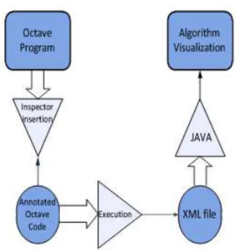
When displaying an algorithm is launched two different drawings: the first one has to draw some standard elements that are always on the screen (named the ”global” elements) during the visualization of the algorithm. The second one has to draw some elements that are showed only for the current iteration that is being visualized. Those elements will be replaced at the next iteration. That is why one is able to see on the class Diagram that the Algorithm class is linked to the MathObject interface by two different links: an iterationList (that is to mean a list of iteration where an iteration is a list of MathObject), and a global list is just a list of MathObject. A generic schema of all software components can be seen in Fig. 1.

Figure 1: Generic shema of all software components

2.1 Annotation with inspector

functions

The software can display on the screen any type of algorithm that uses some type of mathematical objects that will be detailed in section 2.3. For this, the algorithm coded in Octave linguage, must be changed a second time to allow record data by each iteration. This data is encapsulated in an XML file.

Two Octave functions, already defined, are added to the Octave code:

init_global() end_global()

These functions are to generate the early part of “global” algorithm, i.e., all elements that appear on the screen from iteration to iteration. For each iteration, other functions are used:

init_data() end_data() init_iteration()

init_iteration_with_information() end iteration()

The init_data is called on the beginning of a list of iterations. This function will be followed by a series of successive calls of init_iteration

function (with or without information) to declare the beginning of a new iteration and a call of

end_iteration function to complete the

can call the end_data function to close the iterations list.

Finishing the iteration annotation it is time to declare the mathematical objects that appear in this iteration. To do this, the following functions are available in Octave:

new_curve new_ellipse new_circle

new_curve_with_parameters new_integral

new_integral with parameters new_parameter

new_point2d new_point3d new_vector

end_curve_with_parameters end_integral_with_parameters

The Octave basic function should be amended to bring up a parameter file_id as the first parameter of the function. This file_id is the file identifier for the XML backup of the execution of the algorithm. This file identifier is created automatically by GraSMA that will itself launch Octave script with this parameter.

If we wish to run the script manually in Octave (it means in GNU Octave), you must have an identifier file (see fopen function in Octave).

All these Octave functions simply write lines of XML in a file. Finally the XML file follows the document type definition (DTM) that enables to be understood by the Java code.

2.1.1

Example of code instrumentation

We present below the sequence of procedures done for the graphical representation of the Newton-Raphson method.

The end users (students and teachers) are not concerned with code annotation; they just chose the algorithm and watch the generated visualizations.

In this approach, code instrumentation is performed by us in each Octave algorithm. It occurs only once throughout the software lifetime. Octave inspector function calls are added to code in order to register in the XML file ”what is happening”.

We start first by changing the header function to add a new argument file_id.

As an example, we are going to present the basic Newton-Raphson in Octave. The original implementation of this method is:

function[x, res,

nbit]=nle_newtraph(f, df, x0, itmax, tol, varargin)

x=x0; nbit = 0; err=tol+1;

fx= feval(f,x,varargin{ : }); if fx==0;

x=x0; res=0; nbit=0; return

end

while err > tol & nbit <= itmax aux = x;

fx = feval(f,x,varargin{ : }); dfx = feval(df,x,varargin{ : });

x = x−fx/dfx;

err = abs(aux−x);

nbit = nbit+1; end

res = feval(f,x,varargin{ : }); if nbit > itmax

printf( [”nle_newtraph stopped without converging to the desired tolerance”,…

”because the maximum number of iteration was reached .\n”] );

end

endfunction

The programming user must decide what he wants to display on the screen. Let’s imagine that he wants to show the target function

f x

( )

Then, before the first iteration of the algorithm, we declare the elements that will be global, i.e. the mathematical elements that will be continuously displayed on the screen. The functions

init_global and end_global must imperatively be called even if the list of elements inside is empty:

Init_global(file_id); put what you want here

for example: new curve (file_id, f); end_global(file_id);

After the declaration of global elements,

init_data function is called in order to prepare the annotation of the iterations. Next, at each iteration we will find at first the init_iteration call (or

init_iteration_with_parameter, which can

the end of the list of iterations, a call to end_data

function is necessary.

Finally, it remains only to make a call to

init_error and end_error before closing the data tag (end_data). One can put a list of errors (new_error_point) after the call to init_error. We show the last modification of Octave code, including all the inspector function calls needed to retrieve all the information we want to visualize:

function[x, res, nbit] =

nle_newtraph(file_ide, f, df, x0, itmax, tol, varargin)

x=x0; nbit = 0; err=tol+1; oldvect=0;

fx= feval(f,x,varargin{ : }); init_global(file_id)

new_curve(file_id,f) end_global(file_id) init_data(file_id) if fx==0;

init_iteration(file_id) x=x0; res=0; nbit=0; end_iteration(file_id) end_data(file_id) return

end

while err > tol & nbit <= itmax init_iteration(file_id,’Info test’) aux = x;

fx = feval(f,x,varargin{ : }); dfx = feval(df,x,varargin{ : }); dim=2;

x = x−fx/dfx;

new_vector(file_id,dim,x,0,aux,fx,’t rue’,’magenta’,’normal’)

new_vector(file_id,dim,x,0,x,1,’tr ue’,’black’,’dotted’);

if (oldvect !=0)

new_vector(file_id,dim,oldvect,0,o ldvect,1,’true’,’black’,’dotted’); end

oldvect=x;

err = abs(aux−x);

nbit = nbit+1;

init_iteration(file_id,’Info test’)

end

res = feval(f,x,varargin{ : }); init_erro(file_id)

end_erro(file_id) end_data(file_id) if nbit > itmax

printf( [”nle_newtraph stopped without converging to the desired tolerance”,…

”because the maximum number of iteration was reached .\n”] );

end

endfunction

2.2

Document type definition

Document Type Definition (DTD) is a structure of mark-up declarations that defines a document type for SGML-family languages (SGML, XML, HTML). A DTD is a kind of XML schema.

DTDs use a brief formal syntax that declares the structure and the elements and its attributes of one type of document. Each case of the DTD will follow the same organization and it has the same elements. Part of the DTM used is:

<!ELEMENT algorithm (global, data, error)

<!ATTLIST algorithm name NMTOKEN

#REQUIRED > < !ELEMENT c i r c l e

EMPTY >

<!ATTLIST algorithm type NMTOKEN #REQUIRED >

<!ATTLIST circle EMPTY>

<!ATTLIST circle color (black | magenta | yellow | white | blue | red) #IMPLIED>

<!ATTLIST circle radius NMTOKEN #REQUIRED> < !ATTLIST c i r c l e r a d i u s NMTOKEN #REQUIRED >

<!ATTLIST circle x NMTOKEN #REQUIRED>

<!ATTLIST circle y NMTOKEN #REQUIRED>

<!ELEMENT curve (parameter*)> <!ATTLIST curve color (black | magenta | yellow | white | blue | red) #IMPLIED >

<!ATTLIST curve value CDATA #REQUIRED>

<!ELEMENT data (iteration+)> <!ELEMENT error EMPTY >

<!ELEMENT global (circle | curve | integral)* >

…

2.3

Visualization of mathematical

objects

The fundamental mathematical objects that we can visualize are: vectors, lines, curves (functions), integrals, circles, ellipses and 3D surfaces. Each of these objects corresponds to a Java class that implements the interface MathObject.

<integral value=”@(x) sin(x)”

color=”green” lowerbound=”−2”

upperbound=”8”> </integral>

The display of integrals was necessary to see the evolution of the Simpson method (Fig. 2), used in numerical analysis, for numerical integration. The first attempt to draw the integrals was based on polygons (because the polygons are one of the basic designs of OpenGL). This was not conclusive because the full draw on the basis of a polygon is possible only if, on the interval over which the integral is calculated, the function does not change its sign. So we used even more basic integrals: using only lines, and different colours that work in all cases. Use 15-point type for the title, aligned to the center, linespace exactly at 17-point with a bold font style and all letters capitalized. No formulas or special characters of any form or language are allowed in the title.

Figure 2: Visualization of the Simpson’s method.

3 GRASMA UTILIZATION

At the opening of GraSMA system, 3 choices are possible: (1) Display of an algorithm that is already registered ; (2) Create a new view of an algorithm that is already octave changed; (3) Import an existing XML file that corresponds to a previous DTD and which is therefore possible to display it on the screen.

In the case (1), you have just to click on the left list, on the algorithm, previously implemented, of your choice. In the case (3), one simply has to click on Files in the menu and then on Import to select the XML file.

In the case (2) of creating a new view of an algorithm already changed in Octave, the process is more complex. First we select Files, then New, and

it simply shows the steps on a new window. In this stage the completion of function parameters is done: - The parameter Algorithm_Type can take any value (it is no longer necessary, this setting may therefore, in the future, never to be asked – there is just for compatibility).

- If we need to refer a function, we must think about writing this function in Octave format (for example @(x) sin(x) for the sinus function).

The Fig. 3 illustrates the case of the call to Newton-Raphson method applied to the function

f x

( )

=

x

approximation

x

₌

1

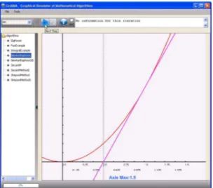
Figure 3: Example of a call to Newton-Raphson method.

Once this information is supplied, the algorithm visual representation appears on the application left side.

The user interface is very simple with icons for: -Go to the next iteration

-Go to the previous iteration

-Make the animation of the algorithm

corresponds to the approximate solution obtained by the tangent function (straight pink) in the previous iteration.

Figure 4: First iteration of Newton-Raphson method.

Figure 5: Second iteration of Newton-Raphson method.

We can increase or decrease the zoom level of the visualization by clicking with the left button of the mouse.

4

GRASMA IMPROVEMENTS

We are planning to add new functionalities to GRASMA. Currently we are working in the automatic annotation of Octave code by means of a compiler that generates annotated code. Other current issue is the development of a website that enables the online access to Grasma.

4.1 Automatic code instrumentation

The main idea is to turn Grasma easily adaptable to other algorithms. As these algorithms are implemented in Octave language and we can extract information in run-time in order to visualize the execution process. For that, a language processor will be used to automatically annotate Octave programs with inspector functions. Till now, this task was performed manually for each algorithm but with this new front-end, Grasma can generate visualizations of any algorithm coded in Octave without modifying manually the source code. To implement code instrumentation [CBHP09] we insert inspection functions (or inspectors) in

strategic places of a program to capture its execution flow. The information extracted along this

inspection can be used to show different views to help understanding program behavior. This is a well known technique for Program Comprehension. To define a strategy to annotate the source code we have to know: which information we need to extract; and what are the strategic points in the source code. To answer these questions we conceptualize the program execution process as a state machine (SM). The input values represent the initial state and the final state can be represented by the variable values after execution. The intermediate states are

represented by the variable values reached during the program execution.

The transition between states is carried out through the octave program functions. The values reached in each algorithm step with be saved internally to produce evolution graphical visualizations.

To implement this strategy we need to build a parser for the source language extended with semantic actions. These actions insert into the program new statements that will allow to trace the state and the transitions.

These tools are based on the language grammar and they allow specifying the automatic recognition and transformation of the program written in that language. In our case the language to be recognized is Octave and the transformation consists in adding the inspector functions.

4.2 WebGRASMA

We are developing a website for the application GRASMA which display the algorithms created on the Canvas by the Java application by parsing the XML files.

Java application extracts the information out of the XML files, by parsing them, and draws the algorithms on the Canvas according to the retrieved information.

For achieving mentioned task, we made use of HTML and Java Servelet technology to create the desired website.

Figure 6: Snapshot of the Grasma website.

REFERENCES

Balsa, C., Alves, L., Pereira, M.J., Rodrigues, P.J. 2010. Graphical Simulator of Mathematical Algorithm (GraSMA). In Teaching and Learning 2010, Advances in Teaching and Learning Research. IASK.

Berón M., Henriques P. R., Pereira M. J. V., Uzal R., 2007. Static and Dynamic Strategies to Understand C Programs by Code Annotation, In OpenCert'07, 1st Int. Workshop on Fondations and Techniques for Open Source Software Certification.

Ramalho J. C, Henriques P. R, 2002. XML & XSL: da teoria à prática. FCA Editor. Lisbon, 1st Ed.

Cadenhead R. and Lemay L., 2007. Teach Yourself Java 6 in 21 Days. Sams, 5th Edition.

Shreiner D., 2009. OpenGL Programming Guide: The Official Guide to Learning OpenGL, Versions 3.0 and 3.1. Addison-Wesley Professional, 7th Edition.

[CBHP09] Daniela da Cruz and Mario Béron and Pedro Rangel Henriques and Maria João Varanda Pereira, Code Inspection Approaches for Program Visualization, Acta Electrotechnica et Informatica, Linus Michaeli, Faculty of Electrical Engineering and Informatics, Technical University of Kosice, Slovakia, 2009, Jul-Sep, 9(3), 32-42, ISSN: 1335-8243.

[ASU86] A. V. Aho, R. Sethi, and J. D. Ullman. Compilers Principles, Techniques and Tools. Addison-Wesley, 1986.

[LMB92] J.R. Levine, T. Mason, and D. Brown. Lex & Yacc. Ed. Dale Dougherty. O’Reilly & Associates Inc., 1992.

[Ter99] Terence Parr. Practical computer language recognition and translation – a guide for building source-to-source translators with antlr and java.

http://www.antlr.org/book/index.html, 1999.

[HVMLGW05] Pedro Henriques, Maria Jo˜ao Varanda, Marjan Mernik, Mitja Lenic, Jeff Gray, and Hui Wu. Automatic generation of language-based tools using lisa system. IEE Software Journal, 152(2):54–70, April