A
N
A
NALYSIS OF
Q
UIT AND
D
ISMISSAL
D
ETERMINANTS BETWEEN
1988
AND
1999
USING THE
B
IVARIATE
P
ROBIT
M
ODEL
V
ERÔNICA
I
NÊS
F
ERNANDEZ
O
RELLANO
Setembro
de 2010
T
T
e
e
x
x
t
t
o
o
s
s
p
p
a
a
r
r
a
a
D
D
i
i
s
s
c
c
u
u
s
s
s
s
ã
ã
o
o
Os artigos dos Textos para Discussão da Escola de Economia de São Paulo da Fundação Getulio
Vargas são de inteira responsabilidade dos autores e não refletem necessariamente a opinião da
FGV-EESP. É permitida a reprodução total ou parcial dos artigos, desde que creditada a fonte.
Escola de Economia de São Paulo da Fundação Getulio Vargas FGV-EESP
Determinants between 1988 and 1999
using the Bivariate Probit Model
*Veronica I. F. Orellano** Paulo Picchetti***
Abstract
Excessive labor turnover may be considered, to a great extent, an undesirable feature of a given economy. This follows from considerations such as underinvestment in human capital by firms. Understanding the determinants and the evolution of turnover in a particular labor market is therefore of paramount importance, including policy consider-ations. The present paper proposes an econometric analysis of turnover in the Brazilian labor market, based on a partial observability bivariate probit model. This model consid-ers the interdependence of decisions taken by workconsid-ers and firms, helping to elucidate the causes that lead each of them to end an employment relationship. The Employment and Unemployment Survey (PED) conducted by the State System of Data Analysis (SEADE) and by the Inter-Union Department of Statistics and Socioeconomic Studies (DIEESE) provides data at the individual worker level, allowing for the estimation of the joint prob-abilities of decisions to quit or stay on the job on the worker’s side, and to maintain or fire the employee on the firm’s side, during a given time period. The estimated param-eters relate these estimated probabilities to the characteristics of workers, job contracts, and to the potential macroeconomic determinants in different time periods. The results confirm the theoretical prediction that the probability of termination of an employment relationship tends to be smaller as the worker acquires specific skills. The results also show that the establishment of a formal employment relationship reduces the probabil-ity of a quit decision by the worker, and also the firm’s firing decision in non-industrial sectors. With regard to the evolution of quit probability over time, the results show that an increase in the unemployment rate inhibits quitting, although this tends to wane as the unemployment rate rises.
Keywords: Turnover, Determinants of quits and dismissals and bivariate probit model.
JEL Codes: C35, J23, J24, J41.
*
Submitted in April 2003. Revised in October 2004.
**
E-mail: [email protected]
***
1. Introduction
The present paper provides an empirical analysis of quit and dismissal deter-minants. Therefore, it sheds some light on the determinants for labor turnover and its evolution in the analyzed time period (1988-1999).
The high labor turnover observed in Brazil1 is impressive and encourages the
development of empirical studies, such as those by Barros et al. (1999b), Bar-ros et al. (1999a), Corseuil et al. (2002) and Gonzaga (2003). The latter study is an in-depth discussion about the Brazilian employment protection legislation and the effectiveness of its incentive mechanisms in the reallocation of workers. This study contributes to the existing debate over the causes of excessive labor turnover in Brazil, having as major contribution the distinct analysis of quits and dismissals, based on the information given by workers about whose initiative it was to terminate the employment contract. This analysis was possible thanks to the information obtained from PED/SEADE/DIEESE. In this context, we also sought to investigate the effect of changes in the Brazilian labor market regulation – implemented in November 1988 by the new Constitution2– on the probabilities
of quits and dismissals.
PED (Employment and Unemployment Survey) data were collected at the in-dividual level, which allowed for the correlation test through a cross-sectional analysis, using the information available about each individual and his jobs. Such tests were performed using the estimation of a bivariate probit model with partial observability. The proposed estimation procedure is based on the joint model-ing of the utility maximizmodel-ing behavior, involvmodel-ing both firms and employees. The econometric model and the data are described in Sections 1 and 2, respectively.
Section 3 describes each covariate used for the estimations, and discusses their inclusion based on the economic theory. This is done for the characteristics of workers and firms (and of the job contract as well), and for the variables that indicate changes in the macroeconomic environment. This includes a discussion about the possible effects produced by a change in the employment protection legislation on the probabilities of quits and dismissals.
Section 4 shows the results obtained with the econometric tests. The results were stratified according to sectors of economic activity, which enables the com-parison between the statistically significant variables for the determination of quit and dismissal probabilities in each sector.
The last section concludes.
1
A manifestation of high turnover would be the large percentage of workers who do not stay on their jobs for two years. Considering only those workers with a formal job contract, the average of this percentage in Brazil amounted to 48.6% between 1990 and 2000, according to the data available from theAnnual Records of Social Information(RAIS).
2
2. Proposal for the Empirical Study: The Bivariate Probit Model
Poirier (1980) regards the bivariate probit model as ideal to analyze situations in which two agents have to individually make a binary choice, and these choices are correlated with each other. For instance, the author presents a situation analyzed by Gunderson (1974), in which the probability of a trainee being hired by the firm which provided the training course was estimated. In this situation, after the training period, the firm should decide whether it would hire the trainee. And the trainee should decide whether he wants to be hired by the firm.
The problem we want to analyze in this study is quite similar to the “trainee case” presented by Gunderson (1974) and Poirier (1980). In this study, employees are observed during a given month of the sample period, and then observed again one year later. In the second observation, the employment relationship may have been maintained or broken by any of the parties, or even broken by both parties. Thus, the idea is that over one year of observation, the firm should decide whether it would maintain the employment relationship. The employee, in his turn, should decide whether to quit or not. Just like in the trainee case, these decisions are correlated.
As Poirier (1980) puts it, the modeling of this situation becomes clearer after placing the problem in an analytical framework in which the two decision-making agents maximize their utility functions.
The firm’s binary choice is represented by yf = 0,1 (where 1 refers to the
maintenance of the employment relationship and 0 refers to the dismissal of an employee); whereas the employee’s choice is represented byye= 0,1 (where 1 refers
to the decision to keep the job and 0 refers to his decision to quit). As previously mentioned, these decisions concern a one-year period. Considering vectorW, with fixed observable characteristics of each firm, each employee and each employment relationship, we assume utility functions of the form:
Uf0=gf0(W, y∗e) +ηf0 (1)
Uf1=gf1(W, y∗e) +ηf1
for the two possible choices made by the firm. Analogously, employees presumably have utility functions of the form:
Ue0=ge0 W, y∗f
+ηe0 (2)
Ue1=ge1 W, y∗f
+ηe1
where, forj =f, eandi= 0,1, we have that: gjiare deterministic functions;ηji
are unobservable random factors; and eachy∗jis equal to (Uj1−Uj0), representing
It should be noted that these functions involve an important hypothesis. This hypothesis posits that the utility an agent attributes to each of his options de-pends on the other agent’s “preference.” This means that the model deals with the hypothesis that each agent perceives, at least in part, the other agent’s “pref-erence,” and this influences his own decision. This hypothesis is supported by lines of research discussed in Section 3, as they show that each agent involved in an employment relationship needs to guarantee that the other party is also com-mitted. Regardless of theoretical developments, we must say that this idea is quite intuitive. As Ehrenberg and Smith (1994, pg. 340) put it “While we may talk of a quit as “worker-initiated,” the fact that an employer did not choose to take steps to retain potential quitters would seem to imply that the employer believed keeping them was not worth the cost.”
Following Poirier (1980), we assume that:
gf1(W, y∗e)−gf0(W, y∗e) =γfy∗e+Xδf (3)
ge1 W, yf∗
−ge0 W, y∗f
=γey∗f+Xγe
ηf1−ηf0=ǫf
ηe1−ηe0 =ǫe
whereX is a covariate vector;δf δe, are vectors of unknown parameters; γf, γe,
are unknown parameters; and
εf
εe
∼N
0,
Wf f Wf e
Wef Wee
Therefore:
y∗
f =γfy∗e+Xδf+ǫf (4)
y∗
e =γey∗f+Xδe+ǫe
which, according to the hypothesis of stochastic utility maximization, means that agentj will choose option 1 if y∗
j >0. That is,yj = 1 ifUj1> Uj0 , for j=f, e.
Defining:
βe= (1−γfγe)−1(δe−γeδf)
βf = (1−γfγe)−1(δf−γf−δe)
νe= (1−γfγe)−
1
)ǫe−γeǫf)
y∗
e=Xβe+νe (5)
y∗
f =Xβf+νf
Thus, two facts allow the interdependence of utility functions of the two indi-viduals. The first one, which was previously mentioned, is that the utility of each individual is specified as being dependent upon the other individual’s “tendency.” The second one is that both unobservable stochastic components are potentially correlated.
Then, even though equations(5) correspond to two separate univariate discrete-choice models, they can benefit from joint estimation, which shows that the bivari-ate model is the most appropribivari-ate. This results directly from higher asymptotic efficiency in a context of maximum likelihood estimation, in the case in which
wf e, wef andρare different from zero.
Assuming the standard bivariate normal distribution as the “link” function, denoted byF(.), we have the bivariate probit model, with log-likelihood function given by:
l(βf, βe, ρ) = N
X
i−1
{yifyie1nF(Xiβf, Xiβe, ρ)
+ yif(1−yie(1−yie1n[φ(Xiβf)−F(Xiβf, Xiβe, ρ)]
+ (1−yif)yie1n(φ(Xiβe)−F(Xiβf, Xiβe, ρ)]
+ (1−yif)(1−yie{1n[ρ(Xi, βf)−F(Xiβf, Xiβe, Xi, ρ)]
+ (1−yif)(1−yie{1n[φ(Xiβf)−F(Xiβf, Xiβe, ρ)]
+ 1n[φ(Xiβe)−F(Xi, βf, Xi, βe, ρ)]}
where φ(.) is the standard univariate normal distribution, andN stands for the sample size.
The likelihood function shown above presupposes that there is enough informa-tion to distinguish each of the four possible combinainforma-tions of decisions made by the firm and by the employee (“keep/stay,” “keep/quit,” “fire/stay,” and “fire/quit”). However, this is not an appropriate hypothesis to deal with the specific situation to be faced in this study. As will be discussed in the next section (data description), the only combination of decisions we can guarantee from the available observation is that in which both the employee and the employer jointly decide to maintain the employment relationship (“keep/stay”), which is directly observed when the employee keeps the same job after one year.
we cannot be sure of what the firm’s decisions would have been by the end of one year. Analogously, if the employee informs us that he was fired, we cannot be sure of what this employee’s decision would have been by the end of one year. The dismissal by the employer might have occurred after a period in which the employee neglected his duties, perhaps while he was looking for another job.
In the specific case of the Brazilian labor market, the labor legislation encour-ages workers to strike a deal with firms, in which case, if they decide to quit, they ask to be formally dismissed (unfair dismissal); thus they are entitled to withdraw the balance of the FGTS account (Seniority Severance Payment Fund account). This casts further doubt on the answer “I was fired” as an actual representation of the employer’s decision.
These considerations support the estimation of the partial observability bivari-ate probit model of Poirier (1980), in which, instead of observingXi,yf i andyei,
i= 1,2, ..., N, we observeXiand zi,i= 1,2, ..., N, where
zi= 1 ifyf i=yei= 1 (6)
zi= 0 in other cases
This means that from the four possible combinations of decisions made by the employee and the firm – “keep/stay,” “keep/quit,” “fire/stay” and “fire/quit” – it is possible to distinguish only the second one from the other three. In this context, the two equations necessarily have to be jointly estimated, given the arguments of asymptotic efficiency. The log-likelihood function is now equal to:
l(βf, βe, ρ) = N
X
i=1
{zi, lnF(Xiβf, Xiβe, ρ) + (1−zi)1n[1−F(Xiβf, Xiβe, ρ)]}
It results directly from the distribution of zi, which is given by:
P r(zi= 1) =pi=Pr(yf i = 1 andyei= 1) =F(Xiβf, Xiβe, ρ) (7)
P r(zi= 0) = 1−pi=P r(yf i= 0 and/oryei= 0) = 1−F(Xiβf, Xiβe, ρ)
If parameters βf and βe are identified, we may estimate the four different
probabilities regarding the four possible combinations of decisions made by the firm and by the employee, using reduced-form equations. A sufficient condition for local identification is that the information matrix of the log-likelihood function above is non-singular (Rothenberg, 1971). This condition, however, does not guarantee global identification.
assumed the partial observability described above. In case of full observability, two additional suppositions were necessary to estimate the model: (i) that the answers given by unemployed individuals about the dismissal initiative are perfectly true and (ii) that when one of the parties decides to end the employment relationship, the other party would have wanted to maintain it. Given these suppositions, we never have the “fire/quit” combination.
The importance of estimating the model by supposing full observability is that the estimated coefficients could be used as initial values for the estimation of the partial observability model. This procedure facilitates the convergence of the partial observability model to the correct equilibrium point.
Another important aspect to be considered regarding partial observability is the loss of efficiency in the estimation. Meng and Schmidt (1985) present some simulation results that confirm the intuitive notion that the larger the proportion of values 1 assumed by variable z in the sample, the lower the cost of partial observability in terms of loss of efficiency. Since, in our case, this corresponds to the proportion of employees that kept the same job for one year, it is encouraging to note that this proportion is relatively high in our sample.
3. Data
The sample consists of data obtained at the individual worker level by the Employment and Unemployment Survey (PED). PED has been carried out every month by the SEADE and DIEESE foundations, since 1984. These databases are used to construct a monthly unemployment rate, among other aggregate in-dicators. Information from January 1985 to December 1999 are available. Ev-ery month, approximately 3,000 randomly selected families are interviewed in the metropolitan region of S˜ao Paulo (RMSP). Each individual is interviewed only once, differently from the rotating panel design that characterizes the PME/IBGE survey. However, PED has a great advantage over the PME: it contains informa-tion about job tenure, both about those workers who were employed at the moment of the interview and about the previous job for those who were unemployed at the time of the interview.
The information about the previous job tenure of those who were unemployed at the time of the interview is only available from February 1988 onwards. For this reason, the econometric estimations cover the period from February 1988 to December 1999.
The sample used in this study consists of individuals who, at the time of the interview, were employed in the same firm for at least one year, also including the individuals who had been unemployed for less than one year at the time of the interview. Individuals aged less than 10 years, domestic and public sector workers were excluded from the original sample.
mean rate for the analyzed period. This is explained by the fact that the selected sample included only workers who had been unemployed for less than one year.
The mean age in the sample is 33 years, 64% are males, 48% are household heads, approximately 40% are formal employees (with a job contract) and the average worker completed 4 years of formal education.3
As expected, the number of terminated employment relationships observed every year tends to be larger in periods in which the unemployment rate rises (table 1).
Table 1
YEAR Evolution of the Open Variation of the total number of unemployment open
terminated rate unymployment
employment rate
relationships(∗)
1988 2,930 7.02
1989 2,683 6.59 -6.1%
1990 3,901 7.21 9.4%
1991 4,545 7.92 9.8%
1992 4,436 9.13 15.3%
1993 3,677 8.68 -4.9%
1994 3,353 8.92 2.8%
1995 3,819 8.95 0.3%
1996 3,805 9.93 10.95%
1997 4,309 10.16 2.32%
1998 4,599 11.67 14.9%
1999 2,576 12.06 3.3%
Source: PED/SEADE-DIESE
(∗) 1 – The number of terminated employment relationships observed every year does not correspond
to the total number of terminated employment relationships associated with the interviewed workers, since, for every interviewed worker, we observe at most one terminated employment relationship every year. 2 – the sample size of PED did not change over the study period.
In addition, table 2 shows the evolution of the number of quits (%) relatively to the total number of employment relationships terminated every year. This percentage tends to be larger in the years in which the level of employment in the metropolitan region of S˜ao Paulo was relatively higher.
3
Table 2
YEAR Quits/total number of Percentage of employed terminated employment workers in PEA
relationships (economically active population) in the RMSP
1988 45% 93.0
1989 47% 93.4
1990 35% 92.8
1991 35% 92.1
1992 32% 90.9
1993 34% 91.3
1994 35% 91.1
1995 31% 91.1
1996 27% 90.1
1997 26% 89.8
1998 24% 88.3
1999 21% 87.9
Table 2 shows a clearly positive relation between the proportion of quits ev-ery year (relatively to the total number of terminated employment relationships) and the level of employment in the RMSP. In the analyzed period, the level of employment in the RMSP fell nearly continuously. More precisely, this level: (i) was quite high until 1989; (ii) fell until 1992; (iii) slightly increased in 1993, being stable until 1995; and finally, (iv) fell again until 1999. The proportion of quits follows the same tendency.
4. Covariates
Before discussing the explanatory variables used for the estimations, we should underscore that one of the major determinants for the possible termination of an employment relationship is the amount of specific training offered to the worker – defined as the type of training that increases the worker’s productivity only in the firm where the training took place. This relation was originally pointed out by Becker (1962), who drew attention to the fact that the investment costs and returns regarding specific training should be shared between the employee and the employer so as to guarantee the continuity of the employment relationship for both parties.4 Becker concluded that there is an inverse relation between investment in
specific training and the probability of termination of an employment relationship.
4
Subsequent empirical studies showed that there is a positive correlation be-tween general and specific training.5 This produces significant differences among
firms regarding the average probability of termination of employment relation-ships, since firms use different technologies of production, which are quite distinct in terms of the average amount of training required from workers. However, the database used in this study contains scarce information about the firms.
The solution was to divide the sample into five sectors – making five separate estimations.6 The different sectors of economic activity differ in terms of the adopted technologies of production, which, in their turn, make them different in relation to the average firm size, to the average amount of training required from workers, and to the average specificity of skills required from workers. The division of the sample into five sectors allows the characteristics of the firms to be more homogeneous in the subsamples.7
Sector 1 includes large industrial companies characterized by a more intensive use of capital.8 Sector 2 includes smaller and less capital-intensive industries
(textile sector, furniture sector, etc...). Finally, sectors 3, 4 and 5 correspond respectively to civil construction, commerce and services.
Table 3 shows the differences between these five sectors regarding the average job tenure and the percentage of workers with a formal job contract.9
5
General training is defined as that which increases the worker’s productivity not only in the firm where the training is offered but also in other firms. For Becker, this type of training should be paid by the worker. Mincer (1988) conducted an empirical study whose results indicate a negative effect of on-the-job training on turnover. For the author, this result may be explained by the positive correlation between general and specific components of on-the-job training.
6
An estimate regarding the whole sample was not included because the intercept dummy variables are not enough to capture important differences between the sectors in the estimated parameters. The only reason to include this estimation is the efficiency gain from the increase in sample size, but this is not relevant in this study, given the size of the samples corresponding to the sectors.
7
A vast literature exists on how the characteristics of jobs and firms influence labor turnover-including not only orthodox models, but also the developments of heterodox economic theory. Econometric studies that assess the relationship between labor turnover and the characteristics of the firms – such as size, technological sophistication and unionization – are quite common. This section does not deal with this issue in detail, due to the paucity of satisfactory data to analyze it empirically.
8
According to the classification presented by Carvalho and Feij´o (1993), the following sectors of processing industry are characterized by the presence of large companies, which offer attrac-tive career opportunities to their employees: metallurgy, transportation materials, paper and cardboard, rubber, chemicals, pharmaceuticals, perfumery beverages and editorial and printing. Orellano (1997) used this classification to test the determinants for quits and dismissals and con-cluded that workers in these sectors have a lower chance to quit their jobs, even if other relevant factors, such as education, qualification level and formal job contract, are controlled.
9
Table 3
More capital– Other Civil Commerce Services intensive industrial construction
industry sectors Average job
tenure 5.3 years 4.2 years 3.9 years 4,years 4.9 years % of workers
with a formal 80.4% 60.3% 31.4% 38.0% 43.7%
job contract
Source: PED/SEADE-DIESE
Table 3 shows large differences between the five sectors regarding the percent-age of workers with a formal job contract. Industry, in general, has a high level of formality concerning employment relationships, followed by the service, commerce and civil construction sectors. This difference may be due, to a great extent, to the fact that industrial firms are usually larger in comparison with firms belonging to other sectors, which allows these firms to be more easily monitored in terms of legal compliance.
Also important is the difference in the level of formality between the most capital-intensive industry and the other industrial firms, which supports the divi-sion of industries into two large subsectors, singling out the most capital-intensive industry. The latter one also has a clearly longer average job tenure.10 It is
in-teresting to note that the less capital-intensive industry does not differ from the commerce and service sectors with regard to the average job tenure, despite the higher level of formality in employment relationships observed in the industry.
In all sectors, the two bivariate probit models (supposing full and partial ob-servability) were estimated – and a set of covariates was included in all estimations. The covariates that indicate job characteristics are concerned with the job that is being analyzed, which we call “reference job.” For individuals who were employed at the time of the interview, the “reference job” would be the job they held at that time. For unemployed individuals, the “reference job” would be the last job, which they left before the interview.
The set of covariates common to the five sectors, which will be discussed ahead, consists of: (i) a dummy variable using number 1 to indicate female workers ( gen-der); (ii) a dummy variable using number 1 to indicate the household head (head); (iii) age (age); (iv) worker’s tenure in the “reference job” (tenure); (v) level of for-mal education determined by the number of school years (educ)11; (vi) a dummy
10
This observation is consistent with the result obtained by Orellano (1997), according to whom workers in the most capital-intensive sectors have a lower chance to quit their jobs, even if other factors, such as education, qualification level and formal job contract, are controlled.
11
variable using number 1 to indicate the workers who had a formal job contract in the “reference job” (contr.); (vii) open unemployment rate (PED/SEADE-DIEESE) published in the month in which the worker left the job, or the mean open unemployment rate during the year in which the workers kept the same job (open unemp); (viii) variation of (deseasonalized) sector GDP in the two months preceding the date on which the worker left the job,12 or the monthly average of
the total sector GDP variation during one year, for workers who kept the same job (gdpvar); (ix) a dummy variable indicating the period after November 1988, when the new constitution made some changes to the Brazilian labor legislation, for workers with a formal job contract and at least three months in the job (dec88); and finally, (x) ten more dummy variables, one for each year, from 1990 to 1999.13
The discussion about the meaning and the expected effect of each of these co-variates is clearer if they are divided into two groups. The first group consists of variables that indicate the workers’ personal characteristics, or the specific charac-teristics of the employment relationship being analyzed. This group includes the first six covariates listed above. The other group, which includes all the remain-ing covariates, consists of variables that indicate changes in the “macroeconomic environment” (including changes in the legislation), or changes in the sector of economic activity analyzed.
Some empirical studies demonstrated that the probability of married men, especially those with children, quitting their jobs is lower than that for single men.14 The opposite occurs with women. Married women, especially those with
children, have a higher probability of quitting their jobs, due to their sporadic absence from work to look after their children and their house.15 Therefore, the
first two covariates included in the estimations seek to capture these effects, the first one indicating the worker’s gender and the second one indicating the worker’s position as “household head,” a position that can also be taken by the woman.
The variable “age” is expected to have an inverse relation with the probability of quitting and being fired. The longer the participation in the labor market (which tends to increase with age), the longer the time this individual had to devote himself to looking for a job and, therefore, the higher his level of satisfaction
12
In case of sectors 3, 4 and 5, only quarterly GDP data were found. Thus, for the first month of each quarter, we associated the GDP variation observed between the two previous quarters. For the last month of each quarter, we associated the GDP variation between the previous quarter and the quarter corresponding to this month. For the intermediate month, we associated the mean of these two variations.
13
The dummy variable indicating a certain year (say, yearX) was constructed in the following manner. Value 1 was associated with individuals who left their jobs in that year and with individuals who were interviewed in that year. The latter ones kept the same job at least for twelve months between the beginning of year (X−1) and the end of yearX.
14
The study conducted by Mincer (1978) is an example. The author explains this result using the highest opportunity costs to change jobs resulting from family bonds. However, one may argue that married men are more averse to the risk of leaving a job only to look for another one.
15
should be. This should occur not only in terms of wage, as presented in the model developed by Burdett (1978), but also with regard to other job characteristics. Thus, the worker’s age should have a positive correlation with the job matching quality, reducing the probability of quitting and the probability of being fired. On top of that, the older the individual, the lower the return expected from the job searching activity, which should also reduce the probability of quitting.
Job tenure is a way to measure the amount of specific skills acquired by an employee. In this case, the idea is simple: the longer a worker stays on the job, the more time he has to acquire these specific skills in relation to the firm where he works. As discussed at the beginning of this section, this should reduce the probability of quitting and the probability of being fired.
Another variable included to measure the amount of specific skills acquired by the worker is his level of formal education. As asserted by Mincer (1994:121), the human capital theory supposes that individuals who achieved a higher level of formal education tend to get a higher amount of on-the-job training – which explains the use of the level of formal education as a way to measure the amount of on-the-job training received by the worker.16 This theoretical result is based on the
hypotheses ofpersistence of investment in human capital and complementarity of investment in human capital. The former supposes that individuals who invested more in formal education will also invest more in training, since the same individual factors that led them to make the first type of investment in human capital will also lead them to invest more in training. The second hypothesis posits that investment in formal education allows individuals to derive more benefits from on-the-job training.
Finally, as the last covariate that indicates specific characteristics of the em-ployment relationship, we included the dummy variable indicating that the worker had a formal job contract (assuming value 1 for workers with a formal job con-tract). Obviously, we expect a negative effect of this variable on the probability of dismissal by the firm, since the formal employment relationship imposes additional dismissal costs (basically, termination notice and FGTS penalty).
Dismissal costs, as well as hiring costs and initial training costs, constitute the fixed costs (or “quasi-fixed costs”) of the labor factor, as they are not proportional to the amount of working hours each employee will devote to the firm, although they are proportional to the number of hired employees. A vast literature exists on the effect of such costs on the dynamics of labor demand, but Oi (1962) was the one who developed this idea. Several models were later developed,17 reaching
the same conclusion that fixed labor costs reduce the oscillation in labor demand
16
The use of the level of formal education as a way to measure the amount of specific skills acquired by the worker requires the additional hypothesis that processes of job training always have some specificity with regard to the firm where they take place – which was discussed at the beginning of this section and is advocated by Doeringer and Piore (1971) and Mincer (1988).
17
– reducing the volume of hirings in periods of growth and the volume of dismissals in periods of recession. Thus, these models suppose that higher dismissal costs imply lower probability of dismissal by the firms, as the employment relationships would be on average more stable in a context with higher costs.
A priori, we also expect an inverse relation between the variable formal job contract(which indicates the formal employment relationship) and the probability of quitting. The fact is that the formal employment relationship offers benefits to the worker (such as welfare, paid vacations, maternity leave, termination pay in case of unfair dismissal, among others). These advantages are highly valued by workers and, therefore, should reduce the probability of these workers quitting their jobs. This conclusion has already been confirmed by empirical tests.18
Now shifting to the group of variables that indicate changes in the “macroeco-nomic environment” or changes in the analyzed sector, the first one we have isopen unemployment (open unemp). The influence of this variable on the probability of quitting is formalized in job search models such as that by Barron and McCafferty (1977), which results in a function that determines the quit rates. According to this model, the level of labor demand is an exogenous variable that influences the individual decision of each worker to search for a job. The rise in labor demand increases the expected net return from the job search, then, the total number of quits responds positively to an increase in the level of labor demand and negatively to a reduction in this level. This generates an inverse relation between unemploy-ment rate and the probability of quitting, which was corroborated in empirical studies such as that carried out by Mincer (1988).19
The unemployment rate can also be viewed as a relevant variable to the deci-sions of firms to fire employees, however, should have a positive relation with the probability of dismissal by the firm, contrary to what occurs with the probability of quitting. The idea is that the firm, when deciding to fire employees, observes the available information about economic activity. The higher the unemployment rate in the previous period, the higher the probability of dismissal by the firm should be.
At this point, it is important to note that the unemployment rate being as-sociated with the workers who left their jobs (quit or fired) corresponds to the unemployment rate of the month prior to dismissal or quitting. Thus, the effect that is measured is that of the unemployment rate on the probability of firing, and not the other way round.
The variable gdpvar, in its turn, is used to measure the variation of product demand in each sector, since a decrease in the demand for a firm’s product should
18
See Orellano (1997:87).
19
generate an adjustment of production so that this production can restore the firm’s equilibrium (profit maximization). By supposing that employers do not fire employees at the first sign of reduction in sales, seeking first to reduce production by reducing the number of hired working hours, the variablegdpvar is a way to measure the demand for the product in the previous period. Dismissals should occur only in a second moment, after an initial reduction in production – provided that the firm believes in the persistence of this decrease in the product demand.
The previous non-seasonal variation of production was used because the firms expect the seasonal decreases in the demand for the product, knowing that they are followed by recovery in the same year. Therefore, a seasonal decrease in demand should not cause dismissals – especially when the hiring and dismissal costs are significant for the firms. However, if a non-seasonal decrease in the demand for the product occurs and this decrease is seen as persistent, this may result in dismissals after a decrease in production.
As the variablegdpvarindicates previous (non-seasonal) variations in produc-tion, given the arguments presented in the two previous paragraphs, a reduction in this variable (assuming sometimes negative values) is expected to increase the probability of dismissal by the firms.
The inclusion of the variablegdpvaras explanatory variable for the probability of quitting, follows a logic that is quite close to that used to explain the relationship between unemployment and quitting. According to the hypotheses being used, previous (non-seasonal) increases in the product of a sector may imply hirings in the subsequent period. This may especially increase the probability of quits among employees in this same sector– who have already acquired skills which, even if not specific to the firm where they have worked, may be specific to the sector of economic activity.
Getting on with the analysis of covariates that indicate changes in the macroe-conomic environment, we should now discuss the expected effect of the variable dec88, which indicates the period after November 1988 (date on which changes were made to labor legislations by the new constitution) for those workers with a formal job contract and with at least three months on the job.20
The incentive mechanism produced by the Brazilian employment protection legislation is quite complex. For that reason, the potential effects caused by a change in this legislation are often contradictory.
With the new Brazilian constitution, the FGTS penalty charge, which should be compulsorily paid by the firms when they dismiss an employee without good reason, increased from 10% to 40%. Given this increase in the dismissal cost, this change is expected to have lowered the probability of dismissal by the firm for those workers with a formal job contract (and at least three months on the job). On the other hand, the fact that the worker can withdraw the money paid by
20
the firm may represent an incentive for him to force his own dismissal, especially in periods of economic growth. Dismissal would be formally seen as dismissal without good reason, when, actually, the worker has the intention to leave the job. The increase in the FGTS penalty charge to be paid by the firm would therefore encourage workers to leave the job.
However, there is one factor that makes this incentive mechanism even more complex: the worker has the right to withdraw the balance of the FGTS account when he is fired. That is, dismissal by the firm implies that the worker is entitled to withdraw the balance of the FGTS account plus the penalty charge paid by the firm. So, there exists the possibility that the firm and the worker will make an agreement in cases in which the worker intends to leave the job. In this agreement, the firm accepts to fire the worker without good reason so that he can withdraw the balance of his FGTS account, but the worker would have to give the amount corresponding to the penalty charge back to the firm.
The increase in the FGTS penalty charge may have inhibited such agreements, since the short-term gain earned by the worker in cases of agreement is reduced with the increase in the FGTS penalty charge. In addition, the employer may feel more reluctant to accept these agreements, since there is an increased risk of the worker not returning the penalty charge paid by the firm. Given all these factors, it is difficult to accurately predict the effect of the increase of the penalty charge on the decision of workers to leave the job.
There is still another relevant change implemented by the new constitution: the creation of the unemployment insurance for workers with a formal job contract. According to the literature, this change encourages attitudes that lead to dismissal by the firm, in periods of low unemployment rate. However, this effect cannot be considered a consensus among researchers, neither from the theoretical nor from the empirical point of view.
Finally, to conclude the discussion about the set of covariates common to all estimations, we have to explain the inclusion of dummy variables associated with each year in the 1990-1999 period. These “year dummies” aim to control the pos-sible effects produced by other relevant macroeconomic changes, as the Brazilian economy had important changes in the 1990-1999 period, such as stabilization plans and the process of trade liberalization.
Only the estimations relative to the two industrial sectors include an additional covariate – in addition to the set of covariates common to all estimations, as previously mentioned and discussed. This covariate, herein referred to asvolatile, seeks to capture the level of uncertainty in relation to the future in each time period. It is an indicator that measures the volatility of the level of production in each period, which was constructed from the data on production available from FIESP, Federation of Industries of the State of S˜ao Paulo, based on a GARCH model.
dismissal results from the hypothesis that a greater uncertainty in relation to the future (the volatility of the level of production is considered an indicator of uncertainty), reduces the response of firms to the previous changes observed in the product demand. In other words, in a moment of higher volatility, an economic setback should not cause several dismissals in the subsequent period, since firms do not view this setback as permanent (or long-lasting). On top of that, one may argue that, in periods of greater uncertainty, a previous economic expansion does not result in hirings in the subsequent period- thus not inducing quits due to a more fierce competition for labor among firms. Therefore, thevolatile variable is expected to reduce quits and dismissals by the firm.
It is worth noticing that, as will be discussed in the next section, the volatility of production in industry increased significantly after 1994 (in addition to being high in 1990). This increase also corresponds to a change in economy in the 1990s, whose effect will be tested.
The volatile variable was only included in the two industrial sectors for two reasons. One reason is that this measure of production volatility was constructed based on data about the industry provided by FIESP. The second reason is that, in industry, turnover costs for the firms tend to be larger, given the increased costs with training. This makes firms hesitate more before they decide to dismiss employees. Therefore, even with a decrease in the product demand, they can try to avoid dismissal in situations of uncertainty.
5. Estimation results
Table 4, on next page, contains a summary of the estimated coefficients for the covariates included in all estimations – with regard to the bivariate probit model with partial observability.21 It should be highlighted that a coefficient with
a positive sign, for instance, indicates that the covariate reduces the probability of dismissal. This occurs because the dependent variable has to be constructed in such a way that number 1 is associated with those workers who did not leave their jobs during one year of observation.
21
Table 4
Bivariate probit model with partial observability estimated coefficients,(∗) for the set of
covariates common to five estimations
fire Sector 1 Sector 2 Sector 3 Sector 4 Sector 5 equation
gender (fem) NS NS -0.142 -0.051 NS
Head NS NS 0.205 0.083 0.074
Age 0.014 0.023 0.006 0.024 0.022 Educ 0.065 0.072 0.026 0.012 0.087 Tenure 0.004 0.010 0.003 0.003 0.010 Contr. -1.953 -1.056 0.939 0.823 0.428
Open unemp -18.671 -13.540 -0.651 -0.708 -3.831 gdpvar 60.646 48.761 2.254 -0.299 167.399
dec88 3.438 2.587 NS NS 0.696
dum90 -7.228 -6.062 -0.356 -0.194 0.602 dum91 13.106 9.061 0.225 0.536 3.130 dum92 33.996 24.596 0.767 1.382 7.238 dum93 39.890 29.271 1.163 1.392 8.486 dum94 29.709 21.331 1.036 1.310 7.065 dum95 29.238 20.727 1.030 1.278 7.597 dum96 47.449 33.331 1.332 1.751 9.765 dum97 51.846 36.415 1.635 2.023 10.915 dum98 77.493 55.559 2.325 2.777 16.378 dum99 87.678 61.469 3.000 3.708 19.199 Constant 130.871 93.818 5.436 5.439 26.088 quit Sector 1 Sector 2 Sector 3 Sector 4 Sector 5 equation
gender (fem) -0.059(∗∗) NS NS NS NS
Head NS NS 0.312 NS 0.115
Age 0.015 0.025 NS 0.025 0.021
Educ 0.077 0.093 NS NS 0.087
Tenure 0.007 0.012 1.619 4.839 0.010
Contr. 2.408 1.873 NS NS 0.771
Open unemp 2.318 2.573 1.642 5.015 8.505 gdpvar -6.234 -18.372 -4.480 -0.533 -493.311
dec88 -0.743 -0.404 NS NS 0.364
dum90 0.835 0.600 0.176 2.351 -0.460 dum91 -1.494 -2.242 -1.949 -4.094 -10.255 dum92 -3.037 -3.642 -2.498 -6.554 -12.147 dum93 -4.681 -5.514 -4.097 -11.552 -21.218 dum94 -4.012 -4.852 -3.445 -10.965 -20.026 dum95 -3.806 -4.780 -3.813 -11.540 -19.458 dum96 -5.383 -6.463 -4.634 -12.220 -25.162 dum97 -6.356 -7.215 -5.654 -17.250 -27.727 dum98 -8.538 -10.071 -6.656 -18.070 -34.132 dum99 -10.758 -12.696 -8.929 -26.138 -46.737 Constant -16.286 -18.084 -29.236 -90.124 -51.680 Wald test 8600.130 8311.13 1485.86 4236.43 22249.94 Log likelihood -7171.604 -7493.78 -4977.746 -12596.577 -19614.812
(∗) Coefficients significant at 5%
(∗∗) Significance level greater than 5% and less than 10%
As was done in the previous section, when the meaning and expected effect of each covariate were discussed, the results will be presented by dividing the covari-ates into two groups– those that indicate characteristics of the individuals or of the employment relationship; and those that indicate changes in the macroeconomic environment or in the analyzed sector.
of the employment relationship for the “reference job”) had a significant effect, with the expected sign, on all estimations. That is, the longer job tenure reduces the probabilities of quitting or being fired, in all analyzed sectors. This result corroborates that one obtained by Orellano (1997:82), suggesting that, in fact, the longer job tenure results in a larger amount of specific skills, encouraging both parties to keep the relationship stable.
The worker’s formal level of education, measured by variableeduc, as described in the previous section, is also pointed by the theory as an indicator of the amount of specific training received by the worker (in addition to variable tenure), and should therefore reduce the probabilities of quitting and being fired. The estima-tions confirm the hypothesis of reduction in quits for the two industrial sectors and for the service sector. The higher level of formal education of a worker certainly reduces the probability of dismissal by the firm, since the obtained results show that this inverse relationship is significant for all sectors.
The significance of variable educin fire equations indicates that the costs in-curred by the firms for adjusting the demand for labor – as expected – increase with the level of education of the employees. The specific training costs correspond to part of these adjustment costs that should be shared with the employees. Since variableeduc, in the civil construction and commerce sectors, is not significant in quit equations, this suggests low costs with specific training in these sectors, or the inability of firms to share the costs of this training with the employees, avoiding unwanted dismissals – or a low correlation between level of education and specific training.
The variable contr., which is the last variable to indicate a specific character-istic of the employment relationship, had the expected effect on the probability of dismissal by the firm, only in non-industrial sectors. That is, the formal employ-ment relationship reduces the probability of dismissal by the firm, as expected, only in non-industrial sectors. Curiously enough, the opposite occurs in industrial sectors.
On top of that, the variable contr had the expected (significant) effect on the probability of quitting in the two industrial sectors and in the service sector. In these sectors, the formal employment relationship reduces the probability of quit-ting, even when other characteristics of the employment relationship are controlled. This indicates that the benefits obtained by the worker with the establishment of a formal relationship (including the relatively higher job stability) are in fact valued by the worker, reducing his propensity for quitting. In the civil construction and commerce sectors, according to the estimation made, the variable contr has no significant effect on the probability of quitting.
(significant) effect in the quit equation in four sectors – the only exception was the civil construction sector. For the reasons discussed in the third section, the more advanced age of a worker is expected to reduce his probability to quit the job, regardless of the correlation between age and job tenure. The probability of dismissal by the firm should also be lower. Both hypotheses were confirmed by the results of the tests.
Differently from the variable age, the variabledummy which indicates female individuals did not have a significant effect on the probability of dismissal (quitting or firing). The only two exceptions were the fire equations of the civil construction and commerce sectors. In these sectors, the results indicate that women have a higher probability to be dismissed by the firms.
Finally, the variablehead, which indicates the household heads, did not show a significant effect on the probability of dismissal in several sectors. Being a house-hold head reduces the probability of dismissal by the firm in the civil construction, commerce and service sectors, but this does not occur in the industry. Moreover, the results show that being the household head only has the significant effect of reducing the probability of quitting in the civil construction and service sectors.
So, we move on to the analysis of the second group of covariates – which indicate changes in the macroeconomic environment or in the analyzed sector. Here, the first observation is that the unemployment rate had the expected (significant) effect on all estimations. That is, in the five analyzed sectors, a higher unemployment rate, observed in the period prior to the termination of an employment relationship, increases the probability of dismissal by the firm and reduces the probability of quitting on the worker’s side.
The previous sectoral GDP variation (seasonally adjusted) also had the ex-pected effect. The only exception is the fire equation of the commerce sector. In other cases, a positive previous variation of production had the expected (signifi-cant) effect of reducing the probability of dismissal by the firm and increasing the probability of quitting.
Therefore, among the set of covariates included in all estimations, now we only have to analyze the effects of the dummy variables (those which indicate the change in labor legislation and the “year dummies”).
The variabledec88, which indicates the moment of change in the Brazilian labor legislation, had the expected effect of reducing the probability of dismissal by the firm in three sectors, not having a significant effect only in the civil construction and commerce sectors. The effect of this variable on the probability of quitting is not consistent among sectors. The probability of quitting, after the changes in the labor legislation, increases in industry, but decreases in the service sector, not having a significant change in other sectors.
data are available only from February 1988 onwards may have limited the analysis, given the possibility that there might have been an anticipation of the changes in the legislation by the agents. Gonzaga (2003) analyzed the 1982-2002 period using a difference-in-difference methodology and concluded that the increase in dismissal cost reduced labor turnover. Furthermore, he concluded that the increase in the FGTS penalty charge reduced the probability of agreements - in which the initiative of dismissal is taken by the worker, but is formally registered as dismissal by the firm.
When analyzing the “year dummies,” it should be noted that the dummies rel-ative to the 1991-1999 period had significant and consistent effects in all analyzed sectors. One may also observe that in 1990 the probability of dismissal by the firm was relatively higher in four of the analyzed sectors – which is not surprising, given the extremely restrictive adjustment policy implemented. In that year, as expected, the probability of quitting was relatively lower in the same four sectors. The only exception was the service sector.
From 1991 onwards, the probability of dismissal by the firm begins to be rel-atively lower in all sectors, given the control over the unemployment rate – this effect is increasingly stronger after 1995. We may say that the reduction in the probability of dismissal by the firm increases from 1995 on because there is an evident increase in the absolute values of coefficients estimated from 1995 in all sectors.
A possible interpretation for this result could be the firms’ modernization pro-cess – with the adoption of new technologies of production – which most researchers believe occurred in the 1990s due to the trade liberalization. However, the liter-ature on the relationship between technology of production and labor turnover assumes that technological modernization should also reduce the probability of quitting. Nevertheless, this is not what “year dummies” indicate in quit equations. They show an increase in the probability of quitting in the 1991-1999 period, with other factors being controlled.
Table 5
Year GDP(∗) GDP variation rate in Open unemployment rate in
S˜ao Paulo the Metropolitan Region of S˜ao Paulo (∗∗)
1991 100,14 7,917
1992 95,99 -4,14% 9,133
1993 103,97 8,31% 8,683
1994 111,20 6,95% 8,925
1995 113,42 2,00% 8,950
1996 115,84 2,13% 9,933
1997 119,49 3,15% 10,158
1998 115,47 -3,36% 11,667
1999 110.22 -4,55% 12,058
(∗) Source = FIPE macrodata (∗∗) Source = PED/SEADE-DIEESE
Between 1991 and 1993, the GDP oscillates, decreasing and increasing, then continuously increasing until 1997. The open unemployment rate – unlike the GDP, as would be expected –, increases and drops again between 1991 and 1993. However, despite the (modest) GDP increase in the 1993-1997 period, we observe an increase in the unemployment rate throughout these years.
As mentioned in the third section, the use of the open unemployment rate as one of the variables that can explain the probability of dismissal by the firms presupposes that the unemployment rate of a given period provides employers with information about the level of economic expansion. This information would be used by firms in the subsequent period as a way to decide whether they should hire or fire employees. In fact, as previously seen, the results confirm that the open unemployment rate of a certain period increases the probability of dismissal by the firm in the subsequent period. Nevertheless, as the unemployment rate rises even in the presence of GDP growth, the dismissal by the firm should actually be less probable. This may be an explanation to the increasing reduction in the probability of dismissal by the firm observed in the “year dummies” after 1995.
Differently from what occurs with the positive relationship between unemploy-ment and the rate of dismissal by the firms, the expected inverse relation between unemployment and quit rates does not result from the hypothesis that unemploy-ment is an indicator of aggregate demand. The variable that really matters when workers have to decide whether to quit or not is the unemployment rate. Thus, theory posits that the growing increase in the unemployment rate throughout the 1990s should reduce the probability of quitting - which was confirmed by the results obtained with the estimates.
rates in the 1990s did not respond negatively to the increase in the unemployment rate in a linear way.
Finally, with regard to the volatile variable, which was not included in all estimations, the results are presented in the statistical appendix at the end of this paper. As expected, this variable reduced the probability of dismissal by the firm in two industrial sectors. Thus, the results suggest that in moments of uncertainty the firms do not respond immediately to a reduction in sales with layoffs, instead, they tend to reduce the number of working hours as a way to decrease production until economic stability can offer reasonable certainty about the future.
The effect of thevolatilevariable on the probability of quitting was not signif-icant in less capital-intensive sectors of the industry, being contrary to that which was expected for the capital-intensive industry, since the increase in the production volatility increases the probability of quitting.
-40 0 40 80 120 160
.000 .002 .004 .006 .008 .010 .012
1986 1988 1990 1992 1994 1996 1998 HEX
TPO
INA GARCH_INAF
Figure 1
Production volatility in the industry of S˜ao Paulo (1985-2000)
In this graph, constructed with data from FIESP, the variable TPO represents the number of employees carrying out production work and the variable INA rep-resents an indicator of the level of activity of S˜ao Paulo’s industries. From 1994 onwards, there is a growing level of activity (with strong oscillations) and a de-crease in the total number of employees in production work.22 The variable HEX,
which indicates the number of extra working hours worked in production, shows an upward trend, and so does the level of activity. The variable GARCH-INAF corresponds to thevolatile variable used for the estimations in this paper. Note that, from 1994 on, industrial production volatility has a relatively higher and more unstable level, especially if compared with the 1991-1993 period.
6. Conclusions
In this study, the analysis of the determinants of dismissals and quits revealed some patterns common to most or all sectors analyzed. These patterns may be observed more clearly in table 4, in the previous section.
Beginning with workers’ personal characteristics, age and level of formal edu-cation showed clear and consistent effects. Age strongly reduces the probability of dismissal and also reduces the probability of quitting in four of the five analyzed sectors. A similar behavior is observed for the level of formal education, thus
22
indicating higher costs for the firm with the hiring and firing of employees who have a better level of education. Moreover, as a higher level of formal education substantially reduces the probability of quitting in the industry and in the service sector, the results suggest that in these sectors the costs with specific training are positively correlated with the level of formal education.
As for the characteristics of each employment relationship, the results obtained show that job tenure reduces the probability of quitting and the probability of dismissal by the firm, in all analyzed sectors. This strongly suggests that the acquisition of specific skills by the worker induces longer employment relationships and greater loyalty from both sides.
It was also observed that a formal employment relationship reduces the proba-bility of quitting, as expected. However, the establishment of a formal employment relationship only reduces the probability of dismissal by the firm in non-industrial sectors, having the opposite effect on the industry, differently from what one would expect.
By analyzing the effects of the variables that indicate changes in the macroeco-nomic environment, we noted that the marginal effect of the open unemployment rate in the five sectors analyzed was consistent with the theories about dismissal and quit determinants. In other words, the unemployment rate of a given period has a negative effect on the probability of quitting and a positive effect on the probability of dismissal by the firm in the subsequent period.
Nonetheless, the results suggest that the increase in the unemployment rate observed in the 1990s had an increasingly weaker effect on the rate of dismissals by the firms. In addition, the quit rates in the 1990s did not respond negatively to the increase in the unemployment rate in a linear way.
The changes to the Brazilian labor legislations made in November 1988 reduced the probability of dismissal by the firm, as expected, not showing a significant effect only in the civil construction and commerce sectors. This result corroborates the conclusions reached by Gonzaga (2003) who, after using the differences-in-differences methodology, concluded that the increase in dismissal costs decreased labor turnover. On the other hand, following our results, the effect of the change in legislation on the probability of quitting is not consistent across sectors.
These results about the effects of institutional changes should be carefully weighted, because the data began to be collected in February 1988, which may limit the analysis, given the possible anticipation of institutional changes by the agents.
Finally, we conclude that an increase in industrial production volatility as a whole, which may be considered a way to measure uncertainty about the future, reduces the responses of industrial firms (dismissals) to variations in the economic activity.
of technological improvement. This is, however, an issue that should be further investigated.
References
Amadeo, E. J., Barros, R. P., Camargo, J. M., Mendon¸ca, R., Pero, V., & Urani, A. (1993). Ajuste estrutural e flexibilidade do mercado de trabalho no Brasil. Anais da Anpec, 2:503–531.
Baltar, P. E. & Proni, M. W. (1995). Flexibilidade do trabalho, emprego e estru-tura salarial no Brasil. Cadernos do CESIT, Texto para Discuss˜ao 15, Unicamp, Campinas, SP.
Barron, J. M. & McCafferty, S. (1977). Job search, labor supply, and the quit decision: Theory and evidence. The American Economic Review, 67(4):683– 691.
Barros, R. P., Corseuil, C. H., & Bahia, M. (1999a). Labor market regulations and the duration of employment in brazil. Instituto de Pesquisa Econˆomica Aplicada – IPEA, Texto para Discuss˜ao Interna 676, Rio de Janeiro.
Barros, R. P., Corseuil, C. H., & Foguel, M. N. (2001). Os incentivos adversos e a focaliza¸c˜ao dos programas de prote¸c˜ao ao trabalhador no Brasil. IPEA, Texto Para Discuss˜ao Interna, 784, Rio de Janeiro.
Barros, R. P., Corseuil, C. H., & Gonzaga, G. (1999b). Labor market regulations and the demand for labor in Brazil. IPEA, Texto para discuss˜ao Interna, 656, Rio de Janeiro.
Beaudry, P. (1994). Entry wages signaling the credibility of future wages: A reinterpretation of the turnover-efficiency-wage model. Canadian Journal of Economics, XXVII(4):884–902.
Becker, G. S. (1962). Investment in human capital: A theoretical analysis.Journal of Political Economy, pages 9–49.
Becker, G. S. (1964). Human capital: A theoretical and empirical analysis, with special reference to education. Columbia University Press, New York.
Burdett, K. (1978). A theory of employee job search and quit rates.The American Economic Review, 68(1):212–220.
Cacciamali, M. C. (1992). Mudan¸cas estruturais e na regula¸c˜ao do mercado de trabalho no Brasil nos anos 80. Texto para Discuss˜ao Interna, 6, IPE/USP.
Chahad, J. P. & Fernandes, R. (2001). Unemployment insurance and transitions in the labor market: An evaluation of Brazil’s program. Texto para Discuss˜ao, S´erie Economia, FEA-USP, Campus de Ribeir˜ao Preto.
Chahad, J. P., Orellano, V. I. F., & Picchetti, P. (2001). A bivariate probit analysis of quits and dismissals. Anais do XXIII Encontro da Sociedade Brasileira de Econometria.
Chang, C. & Wang, Y. (1995). A framework for understanding differences in labor turnover and human capital investment. Journal of Economic Behaviour and organization, September.
Chang, C. & Wang, Y. (1996). Human capital investment under asymmetric information: The Pigovian conjecture revisited. Journal of Labor Economics, 14(3):505–519.
Corseuil, C. H., Ribeiro, E. P., Santos, D., & Servo, L. (2002). Job and worker flows in Brazil. In Menezes-Filho, N. A., editor,Labor Market Dynamics in Brazil. Inter-American Development Bank Research Network, 11th Round, FIPE-USP.
Doeringer, P. B. & Piore, M. J. (1971). Internal labor markets and manpower analysis. D.C. Heath and Company and Heath Lexington books, Massachusetts.
Ehrenberg, R. & Smith, R. (1994). Modern Labor Economics. Harper Collins. Fifth Edition.
Gonzaga, G. (1998). Rotatividade e qualidade do emprego no Brasil. Revista de Economia Pol´ıtica.
Gonzaga, G. (2003). Labor turnover and labor legislation in Brasil. Economia, 4(1). Fall.
Greene, W. H. (1990). Econometrics Analysis. Macmillan Publishing Company, New York.
Gunderson, M. (1974). Retention of trainees: A study with dichotomous dependent variables. Journal of Econometrics, 2.
Hamermesh, D. S. & Pfann, G. (1992). Turnover and the dynamics of labor de-mand. National Bureau of Economic Research, Working paper 4204, Cambridge, MA.
Heckman, J. (1978). Dummy endogenous variables in a simultaneous equation system. Econometrica, 46(6).
Lynch, L. M. (1992). Differential effects of post-school training on early career mo-bility. National Bureau of Economic Research, Working paper 4034, Cambridge, MA.
Menezes-Filho, N. & Picchetti, P. (2000). Os determinantes da dura¸c˜ao do desem-prego em S˜ao Paulo. Pesquisa e Planejamento Econˆomico, 30(1).
Meng, C. & Schmidt, P. (1985). On the cost of partial observability in the bivariate probit model. International Economic Review, 26(1):71–85.
Metcalf, D. (1987). Labour market flexibility and jobs: A survey of evidence from OECD countries with special reference to Europe. In Layard, R. & Calmfors, L., editors,The Fight Against Unemployment: Macroeconomic Papers from the Center of European Studies, pages 51–76. MIT Press. First edition.
Milgron, P. & Roberts, J. (1992). Economics, Organization and Management. Prentice-Hall International, Inc.
Mincer, J. (1978). Family migration decisions. Journal of Political Economy, 86(5):749–773.
Mincer, J. (1988). Job training, wage growth and labor turnover. National Bureau of Economic Research, Working paper 2690, Cambridge, MA, pp. 1–43.
Mincer, J. (1994). Human capital, a review. In Kerr, C. & Staudohar, P. D., editors, Labor Economics and Industrial Relations: Markets and Institutions, pages 109–141. Wertheim publications in Industrial Relations.
Nickell, S. J. (1978). Fixed costs, employment and labour demand over the cycle. Economica, 45(11):329–345.
Nickell, S. J. (1986). Dynamic modles of labour demand. In Ashenfelter, O. & Layard, R., editors, Handbook of Labor Economics, pages 473–522. North-Holland, Amsterdam.
Nickell, S. J. (1995). Labour market dynamics in OECD countries. Discussion and working papers, Institute of Economics and Statistics, Oxford University, November 27th.
Oi, W. (1962). Labor as a quasi-fixed factor. Journal of political economy, 4:538– 555.
Pfeffer, J. & Cohen, Y. (1984). Determinants of internal labor markets in organi-zations. Administrative Science Quarterly, 29(4):550–572.
Poirier, D. J. (1980). Partial observability in bivariate probit models. Journal of Econometrics, 12:209–217.
Ribeiro, E. P. (2001). Rotatividade de trabalhadores e cria¸c˜ao e destrui¸c˜ao de postos de trabalho: Aspectos conceituais. IPEA, Texto para Discuss˜ao 820, Rio de Janeiro.
Rossi-Junior & Ferreira (1999). Evolu¸c˜ao da produtividade industrial brasileira e abertura comercial. Pesquisa e Planejamento Econˆomico, abril.
Rothenberg, T. J. (1971). Identification in parametric models. Econometrica, 39:577–591.
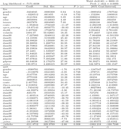
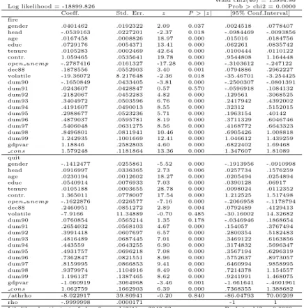
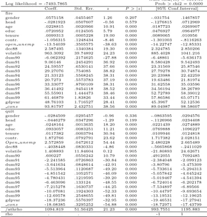
Appendix
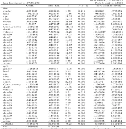
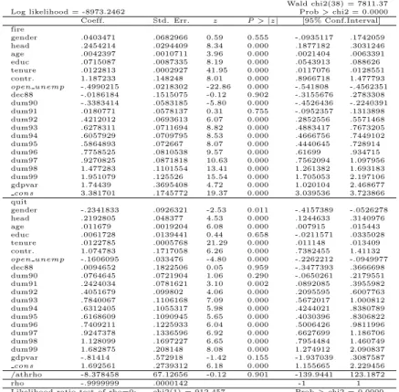
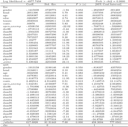
Table A.1 Bi-variate probit model supposing full observability
Table A.2 Bi-Variate Probit Model Supposing Full Observability (Sector 1)
biprobit fire quit gender head age educ tenure contr.Open unempdec88
volatile dum90 dum91 dum92 dum93 dum94 dum95 dum96 dum97 dum98 dum99 gdpvar;
Bivariate probit regression Number of obs = 73689 Wald chi2(40) = 24632.22 Log likelihood = -17096.273 Prob > chi2 = 0.0000 Coeff. Std. Err. z P >|z| [95% Conf.Interval] fire
gender .0352307 .0221263 1.59 0.111 -.008136 .0785975 head -.0416411 .0223384 -1.86 0.062 -.0854234 .0021413 age .0107593 .0009543 11.28 0.000 .0088889 .0126296 educ .0599793 .0049264 12.18 0.000 .0503237 .069635 tenure .0061098 .0001966 31.08 0.000 .0057245 .0064951 contr. 1.53837 .0471837 32.60 0.000 1.445892 1.630849 Open unemp -.3795738 .0162001 -23.43 0.000 -.4113254 -.3478222 dec88 -.0284129 .0474943 -0.60 0.550 -.1215 .0646743 volatile -48.42554 7.737352 -6.26 0.000 -63.59047 -33.26061 dum90 -.1253643 .0414077 -3.03 0.002 -.206522 -.0442066 dum91 .2298491 .040431 5.68 0.000 .1506058 .3090924 dum92 .4585622 .0444684 10.31 0.000 .3714057 .5457187 dum93 .6720309 .0513097 13.10 0.000 .5714656 .7725961 dum94 .7174339 .048891 14.67 0.000 .6216094 .8132585 dum95 .7130776 .0506424 14.08 0.000 .6138204 .8123348 dum96 1.053424 .059353 17.75 0.000 .9370939 1.169754 dum97 1.107757 .0626942 17.67 0.000 .9848788 1.230636 dum98 1.614832 .0789488 20.45 0.000 1.460095 1.769569 dum99 2.046425 .0968333 21.13 0.000 1.856636 2.236215 gdpvar 1.53594 .2611899 5.88 0.000 1.024017 2.047862 cons 2.309571 .1193567 19.35 0.000 2.075636 2.543506 quit
gender -.1262818 .030917 -4.08 0.000 -.186878 -.0656857 head .0827894 .0357241 2.32 0.020 .0127716 .1528073 age .0141213 .0014612 9.66 0.000 .0112574 .0169853 educ .0464904 .0077919 5.97 0.000 .0312187 .0617622 tenure .0059464 .0003355 17.72 0.000 .0052888 .0066041 contr. 1.654448 .0733372 22.56 0.000 1.51071 1.798186 Open unemp -.1250488 .0232873 -5.37 0.000 -.1706911 -.0794065 dec88 -.0798298 .0762391 -1.05 0.295 -.2292557 .0695962 volatile -4.479341 11.21781 -0.40 0.690 -26.46585 17.50717 dum90 .1549682 .0617163 2.51 0.012 .0340066 .2759298 dum91 .2842246 .0554335 5.13 0.000 .1755769 .3928724 dum92 .5074998 .0670707 7.57 0.000 .3760437 .6389559 dum93 .5454405 .0769528 7.09 0.000 .3946158 .6962652 dum94 .5376673 .0697984 7.70 0.000 .400865 .6744697 dum95 .5440824 .0715266 7.61 0.000 .4038928 .684272 dum96 .7672185 .0848635 9.04 0.000 .6008892 .9335478 dum97 .7926086 .0904059 8.77 0.000 .6154162 .9698009 dum98 .9490591 .109203 8.69 0.000 .7350251 1.163093 dum99 1.338152 .1475531 9.07 0.000 1.048953 1.62735 gdpvar -.6809879 .3658443 -1.86 0.063 -1.39803 .0360537